© ESO 2018

1 Introduction

In a recent paper (Lucy 2018; L18), straightforward procedures are proposed for Bayesian model checking.

Because all Bayesian inferences derive from the posterior probability density function Λ(α|D), where α is the parameter vector and D is the data, these tests check the global goodness-of-fit (GOF) to D provided by Λ. The proposed checks take the form of p-values closely analogous to those familiar in frequentist analyses. The first test derives from the ${\chi }_B^2$ statistic (L18, Appendix C) for uncorrelated measurement errors. The second test derives from the ${\psi }_B^2$ statistic (L18, Appendix C.1) for correlated measurement errors.

The need for readily-applied Bayesian model checking procedures has recently been persuasively ponted out by Ford - see Sect. 4.1 in Fischer et al. (2016). Ford attributes the frequent neglect of model checking by Bayesians to the absence of a “neat and tidy” test criterion for Bayesian analyses, in contrast to the χ² criterion for frequentist analyses. For Bayesian model checking, Ford recommends the book by Gelman et al. (2013), which advocates posterior predictive checks.

In Sect. 6.4 of L18, a numerical experiment is briefly reported in which p-values from posterior predictive checking are compared to those derived from the same data with the ${\chi }_B^2$ statistic. Given the importance of establishing the merits of the simpler approach provided by the ${\chi }_B^2$ statistic, this short paper presents the numerical experiment in some detail.

2 Bayesian p-values

In this section, the basics of the p-values to be compared are stated.

2.1 Posterior predictive p-value

On the assumption that χ² is an appropriate test quantity - other possibilities are discussed in Gelman et al. (2013), the steps required to obtain the posterior predictive p-value are as follows:

• 1)

  Compute the posterior probability density function, given by

$$\Lambda (\alpha |D)=\pi (\alpha )\mathcal{L}(\alpha |D)/{\displaystyle \int \pi }(\alpha )\mathcal{L}(\alpha |D)\text{d}{V}_{\alpha }$$(1)

where π is the prior, and $\mathcal{L}$, the likelihood, is given by $$\mathcal{L}(\alpha |D)=Pr(D|\alpha )\propto \exp [-\frac{1}{2}{\chi }^2(\alpha |D)].$$(2)

• 2)

  Randomly select a point α′ from the posterior density Λ(α|D).

• 3)

  Compute a simulated data set D′ at α′ by randomly sampling Pr(D|α′).

• 4)

  Compute and record the values of χ²(α′|D′) and χ²(α′|D).

• 5)

  Repeat steps 2) to 5) ${\mathcal{N}}_{tot}$ times.

The resulting Bayesian p-value is then $$p_B=\mathcal{N}({\chi }^2({\alpha }^{\prime }|D^{\prime })>{\chi }^2({\alpha }^{\prime }|D))/{\mathcal{N}}_{tot}.$$(3)

2.2 p-value from the ${\chi }_B^2$ statistic

Following earlier work (Lucy 2016; L16) on the statistical properties of the posterior mean of χ² , the general form of the ${\chi }_B^2$ statistic is (Appendix C in L18) $${\chi }_B^2(D)={\langle {\chi }^2\rangle }_{\pi }-k$$(4)

where k is the number of parameters and $${\langle {\chi }^2\rangle }_{\pi }={\displaystyle \int {\chi }^2}(\alpha )\Lambda (\alpha |D)\text{d}{V}_{\alpha }.$$(5)

The p-value corresponding to the ${\chi }_B^2$ statistic is derived from the χ² distribution with ν = n − k degrees of freedom, where n is the number of measurements. Specifically, $$p({\chi }_B^2)=Pr({\chi }_{n-k}^2>{\chi }_B^2).$$(6)

The theoretical basis of this p-value is as follows: in the majority of astronomical applications of Bayesian methods, the priors are weak and non-informative. Typically, π(α) defines a box in α-space representing a search volume that the investigator is confident includes all points α with significant likelihood. In consequence, a weak prior has neglible effect on the posterior density Λ and therefore also on any resulting inferences.

In the weak prior limit, Eq. (1) simplifies to $$\Lambda (\alpha |D)=\mathcal{L}(\alpha |D)/{\displaystyle \int \mathcal{L}}(\alpha |D)\text{d}{V}_{\alpha }$$(7)

and the resulting posterior mean of χ² is written as${\langle {\chi }^2\rangle }_u$.

Now, in Appendix A of L16, it is proved that, for linearity in α and normally-distributed measurement errors, $${\langle {\chi }^2\rangle }_u-k={\chi }_0^2$$(8)

where ${\chi }_0^2$ is the minimum value of χ² (α|D). Since, under the stated assumptions, the minimum-χ² solution ${\chi }_0^2$ has a ${\chi }_{\nu }^2$ distribution with ν = n − k degrees of freedom, it follows that, with the extra assumption of a weak prior, the statistic ${\chi }_B^2$ defined in Eq. (4) is distributed as ${\chi }_{n-k}^2$. This is the theoretical basis of the p-value given in Eq. (6).

2.3 p-value from the ${\psi }_B^2$ statistic

The ${\chi }_B^2$ statistic of Sect. 2.2 is appropriate when the measurement errors are uncorrelated. When errors are correlated, χ² (α|D) is replaced by (see Appendix C.1 in L18) $${\psi }^2(\alpha |D)=v^{\prime }{C}^{-1}v$$(9)

where C is the covariance matrix and v is the vector of residuals. The statistic ψ² reduces to χ² when the off-diagonal elements of C⁻¹ are zero – i.e., no correlations.

By analogy with the statistic ${\chi }_B^2(D)$, a statistic ${\psi }_B^2(D)$ is derived from the posterior mean of ψ². Specifically, $${\psi }_B^2(D)={\langle {\psi }^2\rangle }_{\pi }-k$$(10)

with corresponding p-value $$p_{({\psi }_B^2)=Pr({\chi }_{n-k}^2>{\psi }_B^2)}.$$(11)

The theoretical basis for this p-value is essentially identical to that for the p-value derived from ${\chi }_B^2$. If we have linearity in α and normally-distributed errors, then in the weak prior limit $${\langle {\psi }^2\rangle }_u-k={\psi }_0^2$$(12)

and ${\psi }_0^2$ is distributed as ${\chi }_{\nu }^2$ with ν = n − k degrees of freedom.

Note that posterior predictive p-values (Sect. 2.1) can similarly be generalized to treat correlated measurement errors. The quantity ψ² replaces χ² , and the random sampling to create simulated data sets can be accomplished with a Cholesky decompostion of the covariance matrix (e.g., Gentle 2009).

3 Test model

A simple 1-D test model is now defined. This allows numerous simulated data sets to be created so that the p-values computed according to Sects. 2.1 and 2.2 can be compared and any differeces established with high statistical confidence.

3.1 Hubble expansion

The null hypothesis is that the local Universe is undergoing an isotropic, cold Hubble expansion with Hubble parameter h₀ = 70 km s⁻¹ Mpc⁻¹. Moreover throughout the local Universe there exists a population of perfect standard candles of absolute bolometric magnitude M = −19.0. Finally, we suppose that the redshifts z of these standard candles are measured exactly, but that their apparent bolometric magnitudes m have normally-distributed measurement errors with σ_m = 0.3 mag.

3.2 Ideal samples

In order to test p-values when the null hypothesis is correct, we need data sets consistent with the above description of the Hubble flow.

We define the local Universe as extending to z_max = 0.2, so that to a good approximation the geometry is Euclidean. If we suppose the standard candles to be uniformly distributed in space, a sample {z_i} is created with the formula $$z_i=z_{max}{x}_i^{1/3}\text{\hspace{0.17em}\hspace{0.17em}for\hspace{0.17em}\hspace{0.17em}}i=1,2,\dots ,n$$(13)

where the x_i are independent random numbers ∈ (0, 1). The distances of these n standard candles are $$d_i=c{z}_i/h_0\text{\hspace{0.17em}\hspace{0.17em}Mpc}$$(14)

and their measured apparent bolometric magnitudes are $${\tilde{m}}_i=M+5\log d_i+25+{\sigma }_m{z}_G$$(15)

where the z_G are independent gaussian variates from $\mathcal{N}(0,1)$.

The n pairs $({\tilde{m}}_i,z_i)$ comprise a data set D from which the posterior probability density Λ(h|D) of the Hubble parameter h can be inferred. Moreover, the global GOF between Λ(h|D) and D can be tested with the p-values of Sects. 2.1 and 2.2.

3.3 Imperfect samples

In order to test p-values when the null hypothesis is false, we need to modify either the model or the data. If we continue to make inferences based on the Hubble flow defined in Sect. 3.1, we can introduce a violation of the null hypothesis by contaminating the data sample with an unrecognized second class of standard candles with a different absolute bolometric magnitude. Thus the data set D now comprises n₁ pairs $({\tilde{m}}_i,z_i)$ with ${\tilde{m}}_i$ given by Eq. (15) and n₂ pairs $({\tilde{m}}_i,z_i)$ with ${\tilde{m}}_i$ given by $${\tilde{m}}_i=M-\Delta M+5\log d_i+25+{\sigma }_m{z}_G$$(16)

and where n = n₁ + n₂. Thus, the sample is now contaminated with a second population of standard candles that are brighter by Δ M magnitudes. The investigator is unaware of this, and so carries out a Bayesian analysis assuming an ideal sample.

4 Comparison of p-values

The Bayesian p-values defined in Sect. 2 are now computed for simulated data samples derived as described in Sect. 3.

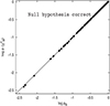Fig. 1 Comparison of p-values. For J = 200 ideal samples Dj, $\log p({\chi }_B^2)$ is plotted against log pB.

4.1 Null hypothesis correct

In order to compare p-values in this case, J independent ideal samples D_j are created as described in Sect. 3.2, and then p-values for each D_j computed as described in Sects. 2.1 and 2.2.

With a constant prior π(h) in the interval (h₁, h₂) with h₁ = 64 and h₂ = 76 km s⁻¹ Mpc⁻¹, the posterior density Λ(h|D_j) is obtained from Eq. (1) with the scalar h replacing the vector α.

The posterior predictive p-value for D_j is computed as described in Sect. 2.1. First, a value h′ is derived byrandomly sampling Λ(h, D_j). This is achieved by solving the equation $${\displaystyle {\int }_{h_1}^{h^{\prime }}\Lambda }(h,D_j)\text{\hspace{0.22em}d}h=x_{\mathcal{l}}$$(17)

where x_ℓ is a random number ∈ (0, 1). Second, an ideal sample D′ for Hubble parameter h′ is computed according to Sect. 3.2. Third, the GOF values χ² (h′|D′) and χ² (h′|D_j) are computed, where $${\chi }^2(h,D)=\sum _1^n{({\tilde{m}}_i-m_i)}^2/{\sigma }_m^2$$(18)

where the predicted apparent bolometric magnitude is $$m_i=M+5\log c{z}_i/h+25.$$(19)

These steps are repeated ${\mathcal{N}}_{tot}$ times with independent random numbers x_ℓ in Eq. (17). The posterior predictive p-value for the ideal sample D_j is then given by Eq. (3).

The corresponding p-value for D_j from the ${\chi }_B^2$ statistic is given by Eq. (4), where $${\langle {\chi }^2\rangle }_{\pi }={\displaystyle \int {\chi }^2}(h,D_j)\Lambda (h|D_j)\text{\hspace{0.22em}d}h$$(20)

with χ²(h, D) from Eq. (18).

The calculations described in Sects. 4.1 and 4.2 are carried out for J = 200 ideal samples D_j , with D_j comprising n = 200 pairs $(z_i,{\tilde{m}}_i)$. In calculating posterior predictive p-values, we take ${\mathcal{N}}_{tot}={10}^5$ randomly selected Hubble parameters h′ for each D_j in order to achieve high precision for p_B.

The results are plotted in Fig. 1. This reveals superb agreement between the two p-values with no outliers. The mean value of |Δlog p| = 2.3 × 10⁻³ confirms that there is almost exact agreement. Accordingly, this experiment indicates that the readily-calculated $p({\chi }_B^2)$ is an almost exact proxy for the posterior predictive p-value p_B , the calculation of which is undoubtedly cumbersome.

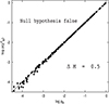Fig. 2 Comparison of p-values for imperfect samples. Each imperfect sample contains 180 standard candles of magnitude M and 20 of magnitude M −ΔM with Δ M = 0.5.

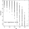Fig. 3 p-values for imperfect samples. Each imperfect sample contains 180 standard candles of magnitude M and 20 of magnitude M −ΔM. For each ΔM, the p values are computed for 200 independent samples.

4.2 Null hypothesis false

In order to compare p-values when p≲0.001, J = 200 independent imperfect samples D_j are created as described in Sect. 3.3. Again ${\mathcal{N}}_{tot}={10}^5$ and n = 200, but now n =n₁ + n₂, with n₁ = 180 perfect standard candles and n₂ = 20 belonging to a second population brighter by ΔM = 0.5 mag. With these changes, the calculations described above are repeated.

The results are plotted in Fig. 2. Because the null hypothesis is false, p-values < 0.01 occur frequently, so that the comparison provided by Fig. 1 now extends to p≲10⁻⁴. However, at these small p-values, the values of p_B are subject to noticeable Poisson noise even with ${\mathcal{N}}_{tot}={10}^5$. Because of this, |Δlog p| = 3.2 × 10⁻², somewhat larger than in Sect. 4.1 but neverthless again confirming the excellent agreement between the two p-values.

In Fig. 3, the behavior of the p-values derived fromthe ${\chi }_B^2$ statistic as a function of ΔM is plotted. With increasing ΔM, the points shift to smaller p-values, increasing the likelihood that the investigator will conclude that the Bayesian model is suspect.

5 Conclusion

The aim of this paper is to investigate the performance of a recenly proposed global GOF criterion ${\chi }_B^2$ for posterior probability densities functions. To do this, a toy model of the local Hubble expansion is defined (Sect. 3) for which both ideal (Sect. 3.2) and flawed (Sect. 3.3) data samples can be created . The p-values derived for such samples from ${\chi }_B^2$ are then compared to the p-values obtained with the well-established procedure of posterior predictive checking. The two p-values are found to be in close agreement (Figs. 1 and 2) throughout the interval (0.0001, 1.0), thus covering the range of p-values expected when a Bayesian model is supported (p≳0.01) to those when the model is suspect (p≲0.01).

Because carrying out a posterior predictive check is cumbersome or even infeasible, the p-value derived from ${\chi }_B^2$ can serve asan effective proxy for posterior predictive checking. Of course, this recommendation derives from just one statistical experiment. Other investigators may wish to devise experiments relevant to different areas of astronomy.

References

All Figures

	Fig. 1 Comparison of p-values. For J = 200 ideal samples Dj, $\log p({\chi }_B^2)$ is plotted against log pB.
In the text

	Fig. 2 Comparison of p-values for imperfect samples. Each imperfect sample contains 180 standard candles of magnitude M and 20 of magnitude M −ΔM with Δ M = 0.5.
In the text

	Fig. 3 p-values for imperfect samples. Each imperfect sample contains 180 standard candles of magnitude M and 20 of magnitude M −ΔM. For each ΔM, the p values are computed for 200 independent samples.
In the text

References

- Fischer, D. A., Anglada-Escude, G., Arriagada, P., et al. 2016, PASP, 128, 6001 [Google Scholar]
- Gelman, A., Carlin, J. B., Stern, H. S., et al. 2013, Bayesian Data Analysis (Boca Raton, FL: CRC Press) [Google Scholar]
- Gentle, J. E. 2009, Computational Statistics (New York: Springer) [CrossRef] [Google Scholar]
- Lucy, L. B. 2016, A&A, 588, A19 (L16) [NASA ADS] [CrossRef] [EDP Sciences] [Google Scholar]
- Lucy, L. B. 2018, A&A, in press, DOI: 10.1051/0004-6361/201732145 (L18) [Google Scholar]