| Issue |
A&A
Volume 614, June 2018
|
|
|---|---|---|
| Article Number | A80 | |
| Number of page(s) | 7 | |
| Section | Galactic structure, stellar clusters and populations | |
| DOI | https://doi.org/10.1051/0004-6361/201732351 | |
| Published online | 18 June 2018 | |
Globular cluster chemistry in fast-rotating dwarf stars belonging to intermediate-age open clusters
INAF – Osservatorio Astrofisico di Arcetri,
Largo Enrico Fermi 5,
50125
Firenze,
Italy
e-mail: This email address is being protected from spambots. You need JavaScript enabled to view it.
Received:
23
November
2017
Accepted:
13
February
2018
Abstract
The peculiar chemistry observed in multiple populations of Galactic globular clusters is not generally found in other systems such as dwarf galaxies and open clusters, and no model can currently fully explain it. Exploring the boundaries of the multiple-population phenomenon and the variation of its extent in the space of cluster mass, age, metallicity, and compactness has proven to be a fruitful line of investigation. In the framework of a larger project to search for multiple populations in open clusters that is based on literature and survey data, I found peculiar chemical abundance patterns in a sample of intermediate-age open clusters with publicly available data. More specifically, fast-rotating dwarf stars (v sin i ≥ 50 km s−1) that belong to four clusters (Pleiades, Ursa Major, Come Berenices, and Hyades) display a bimodality in either [Na/Fe] or [O/Fe], or both, with the low-Na and high-O peak more populated than the high-Na and low-O peak. Additionally, two clusters show a Na–O anti-correlation in the fast-rotating stars, and one cluster shows a large [Mg/Fe] variation in stars with high [Na/Fe], reaching the extreme Mg depletion observed in NGC 2808. Even considering that the sample sizes are small, these patterns call for attention in the light of a possible connection with the multiple population phenomenon of globular clusters. The specific chemistry observed in these fast-rotating dwarf stars is thought to be produced by a complex interplay of different diffusion and mixing mechanisms, such as rotational mixing and mass loss, which in turn are influenced by metallicity, binarity, mass, age, variability, and so on. However, with the sample in hand, it was not possible to identify which stellar parameters cause the observed Na and O bimodality and Na–O anti-correlation. This suggests that other stellar properties might be important in addition to stellar rotation. Stellar binarity might influence the rotational properties and enhance rotational mixing and mass loss of stars in a dense environment like that of clusters (especially globulars). In conclusion, rotation and binarity appear as a promising research avenue for better understanding multiple stellar populations in globular clusters; this is certainly worth exploring further.
Key words: stars: abundances / globular clusters: general / open clusters and associations: general / stars: rotation / binaries: general
© ESO, 2018
1 Introduction
The long-standing problem of multiple populations (MPs) in globular clusters (GCs) is still awaiting for a solution. Briefly, GC stars, which have not undergone classical chemical evolution like in dwarf galaxies, display prominent abundance variations in light elements that often take the form of anti-correlations. The most widely studied anti-correlations are those in C–N, Na–O, and Mg–Al (Kraft 1994; Gratton et al. 2012). Variations are also observed in helium, lithium, flourine, potassium, and s-process elements (Smith et al. 2005; Strader et al. 2015; D’Orazi et al. 2015). Photometry reflects these abundance variations in the form of multiple photometric sequences that are currently not fully explained (Sbordone et al. 2011; Milone et al. 2017).
The observed chemical patterns are generally ascribed to hydrogen burning through the CNO cycle and hotter Ne–Na and Mg–Al cycles (Denisenkov & Denisenkova 1989). Different scenarios were built around different possible polluting stars, such as asymptotic giant branch stars, fast-rotating massive stars, massive interacting binaries, or supermassive stars (Decressin et al. 2007a,b; Ventura et al. 2013; de Mink et al. 2009; Denissenkov & Hartwick 2014). These are collectively known as generational scenarios, because they postulate that an initial stellar generation with normal halo chemistry pollutes the intracluster gas, which in turn forms a second stellar generation with an age difference of ≃3–200 Myr, depending on the scenario. Several other non-generational scenarios or original ideas were put forward, but were less frequently pursued and tested than generational scenarios. Unfortunately, generational scenarios suffer from a series of problems (see Renzini et al. 2015; Bastian & Lardo 2017, for more details) that are not solved to date.
One fruitful line of investigation has been to investigate stellar clusters with different properties such as open clusters (OC) or young massive clusters to place a boundary around the phenomenon in the space of age, mass, metallicity, and compactness (Bragaglia et al. 2012; Krause et al. 2013; Cabrera-Ziri et al. 2016, 2017; Martocchia et al. 2018). In the framework of a larger project to search for MPs in OCs, I collected literature data and found chemical patterns that were impressively similar to those of GC stars in fast-rotating A and F dwarfs in 100–800 Myr OCs. This paper briefly reports and discusses the findings to call the community attention to physical processes that have not been thoroughly explored so far, but might help to explain MPs in GCs.
2 Data
Abundance measurements of A and F dwarfs in five extremely well studied clusters of different ages were collected from the literature, as indicated in Table 1. All measurements of the projected rotational velocities, stellar parameters, and element abundances were obtained from high-quality echelle spectra, with R ≃ 30 000–75 000 and a signal-to-noise ratio (S∕N) ≃ 100–600. The abundance analysis was performed by various teams that used different methods, models, line lists, solar reference abundances, and so on. Whenever possible, I preferred works using similar methods, although offsets of the order of 0.1 dex between one study and the other are always to be expected. All methods were specifically developed for the treatment of fast-rotating stars, are strictly based on spectral synthesis, and the cited papers include the discussion of non-local thermal equilibrium (non-LTE) effects. Different works on the same cluster generally agree with each other within the reported uncertainties and present detailed and satisfactory comparisons with previous literature.
In particular, the Hyades A and F dwarfs were studied by both Gebran et al. (2010) and Varenne & Monier (1999) with comparable outcomes. The Gebran et al. (2010) sample was preferred because of the higher spectral S∕N (200–600) and because the abundance analysis method was the same employed for the chosen Pleiades and Coma Berenices datasets (Gebran et al. 2008; Gebran & Monier 2008). Similarly, the Fossati et al. (2007, 2008) analysis of Praesepe agrees with past work (Hui-Bon-Hoa et al. 1997; Hui-Bon-Hoa & Alecian 1998; Andrievsky 1998; Burkhart & Coupry 1998), but is based on a larger sample with a higher S/N and a more homogeneous analysis with the other selected literature sources.
The final collected sample contains 105 well-known stars with 6 < v sin i < 200 km s−11, all from theHenry Draper catalogue (Cannon & Pickering 1993) and with extremely well studied properties in the literature. The behaviour of the four elements of interest as a function of v sin i is displayed in Fig. 12. Only stars considered as bona-fide members by the respective authors were retained. The samples also contain a few stars in binaries (where the companion does not significantly contaminate the spectra), some δ Scuti variables, several blue stragglers, and several peculiar Am and Fm stars (see Alecian et al. 2013, and Sect. 3.4 for more details). These peculiar stars do not occupy clearly distinct positions in the space of the elements analysed here, with the exception of stars with large [Fe/H] variations, as indicated in Fig. 1, which are suspected or confirmed Am and Fm stars that are affected by strong metallicism. These stars were removed because it is well known that they do not exist in GCs. Theoretically, the effects of diffusion mechanisms are expected to be much smaller (Richard et al. 2002) for population II stars, and this is confirmed observationally (Korn et al. 2007). Iron variations are generally lower than 0.05 dex in the vast majority of GCs (Mucciarelli et al. 2015). Therefore these peculiar stars were removed from the sample and are not considered in the following.
The common conclusion of all the cited studies was that A stars show an increased abundance spread in all elements compared to F stars. At these ages and metallicities, A stars have the tendency to be faster rotators than F stars. Comparisons with diffusion models for F stars (generally those by Turcotte et al. 1998) showed that additional mixing mechanisms must be operating in early-F and in A stars, preventing the expected decrease in light elements and increase in heavy elements. Because the disagreement with models generally increases with v sin i, rotational mixing was proposed by all considered works as the most important of all mixing phenomena, to restore agreement with the observations.
Purely rotational models from the Geneva group (see Lagarde et al. 2012, and references therein) didnot reproduce the observed abundance variations, and predict variations of <0.1 dex in C, N, O, Na, Mg, and Al for these dwarfs. However, rotation does have the potential of competing with diffusion processes, and may also help to explain the peculiar Am star chemistry (Talon et al. 2006). Works from the Montreal group further explored the capability ofturbulent mixing and of mass loss (see Vick et al. 2010; Michaud et al. 2011, e.g.) as competing mechanisms against diffusive processes and found that either can explain observations. This shows that the exact mechanism that counteracts the expected diffusion effects is currently not univocally identified, but there are various equally valid possibilities that are difficult to distinguish observationally.
Selected clusters with basic information and literature source of ages and spectroscopic analysis.
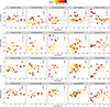 |
Fig. 1 Behaviour of the elements of interest as a function of v sin i. Each row displays a different element and each column a different OC, sorted by age, as annotated. Stars are coloured as a function of Teff. The median [Fe/H] abundance of each OC is represented as a solid green line in the top panels, along with its error range (dashed green lines). Stars with [Fe/H] beyond the normal error range, which are suspected of being chemically peculiar Am and Fm stars affected by strong metallicism, are marked with black crosses. The solar line is plotted in orange. Median error bars are plotted in dark red. |
3 Results
3.1 Bimodal distributions of [Na/Fe] and [O/Fe]
The first surprising result is an apparent [Na/Fe] bimodality in all clusters except Praesepe. This is visible in all figures, but is more noticeable in Fig. 2 (top panels), where the [Na/Fe] histogram is displayed for each of the five OCs. The [Na/Fe] distribution has a spread that is significantly larger than the typical (median) error bar. The peak width is roughly compatible with the typical uncertainties, while the peak separation is generally larger than the typical uncertainties. A Gaussian mixture model fit to the [Na/Fe] distribution with a varying number of components clearly provides the best Bayesian information criterion (BIC) with two Gaussians, except for the Pleiades and Praesepe. Using equal or variable variance models does not change the result because the best-fitting Gaussians have compatible variances in all cases. Generally, the left peak (low [Na/Fe]) contains more stars than the right peak.
A bimodality is also suggested by visually inspecting the [O/Fe] distributions (Fig. 2, bottom panels): two peaks are generally apparent, and their width and separation are compatible with the typical uncertainties. The relative importance of the two visually apparent peaks is generally reversed compared to the [Na/Fe] distributions. However, the data points are less numerous and the histograms noisier: two OCs only, the Pleiades and Coma Berenices, have a higher BIC with two-Gaussian fits than with one-Gaussian fits. Finally, the distribution of [Mg/Fe] shows no clear bimodality.
Unfortunately, I was unable to identify univocally the parameters that govern the bimodality with the sample in hand. Coma Berenices clearly shows a Teff difference between the two peaks (see also Fig. 1), but the range in v sin i is small, and both groups contain stars of varying v sin i. The clear Teff difference between the peaks that is visible in Coma Berenices is not visible in any of the other OCs, except maybe for Ursa Major (see Fig. 1). The hottest stars in Coma Berenices are often classified as Am stars, but in the other OCs, the Am and Fm stars are not confined to one of the two peaks. In the Hyades, stars in binaries often but not always tend to be on the upper sequence, but this is not so clearly the case in the other OCs.
None of the theoretical models mentioned in the preceding section predict this bimodality, if the stellar parameters are the same. Therefore, it is necessary to understand which stellar property assigns stars to each of the two peaks, if the peaks are confirmed to be distinct. Sample size is not the only parameter that needs to be improved to further investigate the matter: it will be necessary to build samples that are as unbiased as possible with respect to the relevant or interesting parameters, such as binarity, peculiarity, variability and pulsation, rotation, temperature, and so on. In particular, the range of Teff covered in Praesepe is smaller than in Coma Berenices, while the range in v sin i is smaller in Coma Berenices than in Praesepe. While some of these differences might be intrinsic and thus unavoidable, we need to have a better understanding of the data properties, and we need more controlled data samples before we can derive any further conclusions.
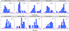 |
Fig. 2 [Na/Fe] distribution (top panels), one for each OC, as a binned histogram (light blue bars) and a generalised histogram (purple lines). The smoothing kernel width was set equal to the bin size, i.e., 0.1 dex. The typical (median) error bar is also reported in each panel. The bottom panels report the same histograms, but for [O/Fe]. |
3.2 Na–O anti-correlation
Figure 3 (top panels) shows the collected data in the Na–O anti-correlation plane, sorted by OC age. The region occupied by GC stars in this plane is represented using the Gaia-ESO data from Pancino et al. (2017). It is important to keep in mind that GC anti-correlations tend to be less extended for more metal-rich and less massive GCs (Carretta et al. 2010; Pancino et al. 2017), and even if OCs had true anti-correlations, they would therefore not be as extended as in GCs. Additionally, and unlike in the GC case, all OCs have some stars in the region of low Na and low O, typically close to solar values3. This cannotbe avoided because the “normal” population in OCs has solar metallicity and no α-enhancement, and this could imply more vertical anti-correlations than in GCs, if they were present.
It appears clear, however, that the distribution of stars in the Na–O plane changes significantly from one OC to the other. The Pleiades and Praesepe stars show no particular resemblance to the GC anti-correlation patterns, except for the bimodality in the Pleaidesdiscussed above.
In Coma Berenices, a clump of stars has values of about solar abundance with Teff ≤ 7000 K (the “normal” stars) and is well separated from a top distribution of hotter stars, with [Na/Fe] confined between 0.3 and 0.7 dex and [O/Fe] spread between solar and –1.0 dex. The high-Nastars cover the same area as the extreme populations observed for example in NGC 2808 (see Pancino et al. 2017, and references therein).
In the Hyades, the stars with v sin i ≥ 50 km s−1 (dark green symbols in Fig. 3) cover a large part of the less extreme Na–O anti-correlation observed in typical GCs: the spread in [Na/Fe] is ≃0.6 dex, the spread in [O/Fe] ≃ 0.5 dex, and the angular coefficient of the anti-correlation is –0.47 ± 0.11, overlapping the reference GC data for the metal-intermediate to metal-rich GCs. In Ursa Minor, the stars rotating faster than v sin i ≥ 50 km s−1 (dark greensymbols in Fig. 3) display a spread of ≃0.5 dex in [Na/Fe] and of ≃0.3 dex in [O/Fe], with an anti-correlation angular coefficient of–2.5 ± 0.4, but the sample is smaller in this case.
To summarise, the fast-rotating stars (v sin i ≥ 50 km s−1) in the Hyades and in Ursa Major display a Na–O anti-correlation, while the hottest stars in Coma Berenices cover the extreme part of the GC anti-correlation, with high Na and a range of O reaching extreme depletion, and a clump of “normal” stars with approximately solar values. These anti-correlations help understanding the inversion of the peak heights (or of the skewness) in the [Na/Fe] and [O/Fe] distributions. The [O/Fe] bimodality in the Pleiades suggests that they might also contain a Na–O anti-correlation; this might be revealed with larger samples. Even considering all the due caveats on sample size and selection function, these patterns do call for further investigation in the light of a possible connection with the MP problem in GCs.
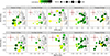 |
Fig. 3 Na-Oanti-correlation plane (top), and the same for Na-Mg (bottom; Al measurements are not available). Reference data for GCs are plotted as grey points (Pancino et al. 2017), and solar abundances as orange lines. Each OC star is coloured based on its projected rotational velocity, and the size of the symbols reflects Teff (hence, mass). Typical (median) error bars are plotted as red crosses. |
3.3 Magnesium depletion
Magnesium is a key element for the MP phenomenon in GCs. It can only be significantly destroyed in the Mg–Al hotter sub-cycles, which require about 80 106 K to become efficient (see Fig. 8 by Prantzos et al. 2007). At the same time, it is not difficult to enhance Al in the Mg–Al cycle: because Mg is so much more abundant, an only modest conversion of Mg into Al is sufficient to significantly enhance [Al/Fe]. For this reason, the fact that the extent of the Mg–Al anti-correlation is extremely variable with the GC mass and metallicity (Pancino et al. 2017) is a very strong constraint on the possible production sites of MPs in GCs, assuming that the Mg–Al cycle is the sole responsible factor for the observed patterns. Mg is also a problem: the very high temperatures required are difficult to obtain in fast-rotating massive stars (Decressin et al. 2007a,b), and only a narrow range of asymptotic giant branch star masses can produce the Mg–Al anti-correlation without destroying too much Na (Ventura et al. 2013; Renzini et al. 2015; Prantzos et al. 2017).
It is therefore very surprising to observe that the hottest stars (Fig. 3, lower panels) in Coma Berenices cover the entire extent of the Mg depletion observed in the most extreme GC stars (well below solar), while at the same time having a high [Na/Fe] (up to 0.7 dex). A stars in Coma Berenices have a typical mass of ~2 M⊙ and thus cannot efficiently activate the Mg–Al cycle in their cores. In the Hyades and in Praesepe, Na-rich stars also cover a range in Mg, with similarly extreme depletion, but in this case, there are also several stars with low Na and a range of Mg that might be chemically peculiar or point to a different chemistry altogether.
It is difficult to measure Al in these stars (I use Na in Fig. 3), and we do not expect significant Al variations in metal-rich GCs (Pancino et al. 2017), but Fossati et al. (2011) did measure Al for six stars in NGC 5460, a poorly studied OC of ≃160 Myr. The result is an Al variation of about 0.3 dex, accompanied by an Mg variation largely exceeding 1 dex. This, among other facts, supports the idea that the low Mg displayed by all OCs examined here is not caused by the Mg–Al cycle burning, but by diffusion and rotational mixing, as described in Sect. 2. It is therefore extremely interesting and worthy of further investigation that the observed chemistry (at least in part) resembles what is observed in the extreme population of GCs. This piece of evidence becomes even more suggestive when considered together with the Na bimodality and the Na–O anti-correlations discussed above.
3.4 Other elements
It would be extremely interesting to study the C–N anti-correla- tion plane as well, but unfortunately, N is not provided in the examined works, except for a handful of stars in Praesepe. The behaviour of carbon with Teff and v sin i is indeed qualitatively similar to that of oxygen, with a similar or more extreme depletion, depending on the OC.
Helium is a key element for MPs in GCs. If the MP chemistry is produced in CNO burning and related hotter cycles, we expect the He abundance to vary as well, with peculiar stars having higher He (see Bastian et al. 2015, and references therein). Helium measurements are not common in the stars analysed here. The theoretical expectations – with all other parameters fixed – predict an increase in He surface abundance with increasing rotational velocity (Ekström et al. 2012). A dedicated He study, for example in correlation with Na and Mg, would be extremely interesting.
Lithiumis also observed to vary in GC stars, anti-correlating with Na or Al (see D’Orazi et al. 2015, and references therein). This is a problem because the proposed polluters do not reproduce the observed chemistry well. All the stars analysed here are hotter than the Li dip, a dramatic drop in Li abundance occurring around 6700 K (Boesgaard et al. 2016), with only the coolest F stars nearing it. Theoretical expectations are that Li is progressively depleted with increasing rotation (Pinsonneault et al. 1989), and the Li dip can be explained as the final outcome of Li destruction mediated by internal mixing and diffusion mechanisms. Unfortunately, the behaviour of Li with rotation for A-type stars is not so well known: the Li line is not observed in fast rotators much hotter than the dip, because it is weak and further weakened by rotation.
Finally, s-process elements (Yr, Zr, Ba) in the studied stars are enhanced up to 0.5 dex and in some cases to 1 dex, and this is especially true for Am stars, which in general display the highest s-process element abundances. This is also in line with what is observed in some GCs.
Moreover, some elements do not vary in the vast majority of GCs, such as the heavier α-elements (Ca, Ti), or most iron-peak elements (Fe, V, Sc, Ni, Cr), which indeed vary in Am and Fm stars and can reach extreme variations, like those shown in Fig. 1 (metallicism). One clear indicator of metallicism in addition to an enhancement in iron-peak elements is a very low scandium abundance (Alecian et al. 2013). These stars are unlikely to have implications for the MP problem, are never observed in GCs, and were not studied here. They are generally slow rotators, in which rotation cannot inhibit the diffusive mechanisms.
In summary, the effect of rotation, or better, of the interplay between rotational mixing and diffusion processes, appears to change all the GC-relevant elements on the surface of these relatively cool stars, and generally in the right direction, even if they are not altered by CNO nuclear processing in these stars at all.
4 Implications for globular clusters
The main results discussed so far can be summarised as follows:
-
1.
Four of the five OCs display an apparent bimodality in [Na/Fe], with the low-Na peak more populous than the high-Na peak (Fig. 2); three out of five OCs pass a BIC test for bimodality.
-
2.
A possible [O/Fe] bimodality is also apparent, although noisier (only two OCs pass the BIC test), with an inversion of peak population (or of skewness) compared to the [Na/Fe] distribution.
-
3.
Two OCs, Ursa Major and the Hyades, display a Na–O anti-correlation of the stars with v sin i ≥ 50 km s−1 (Fig. 3), which explains the inversion of the peak population mentioned before; this suggests that the Pleiades might also contain a Na–O anti-correlation, given that they show an [O/Fe] bimodality.
-
4.
The last OC, Coma Berenices, contains in the high-Na peak stars with a range of O and Mg abundances that reaches the extreme depletion of NGC 2808, and the low Mg is clearly not produced by Mg–Al cycling.
While these results need of course to be verified and further investigated, this is the first detection of a Na–O anti-correlation in OC dwarf stars. Unfortunately, two complications prevent a direct and obvious connection with the GC case. The first is that while rotation appears to be an important ingredient of the observed Na–O anti-correlation and bimodality because only stars rotating faster than v sin i ≥ 50 km s−1 have clear Na–O anti-correlations, the exact ingredient that separates stars into Na-rich and Na-poor is not identified so far (Sect. 3.1). The second is that the observed chemical patterns are too superficial in these stars (10−6–10−4 of the stellar mass, Richard et al. 2002) and are not expected to survive the first-dredge up when they will start ascending the red giant branch, unlike GC stars. This is also confirmed observationally, because OC giants generally do not display Na–O anti-correlations (de Silva et al. 2009; Smiljanic et al. 2009; Pancino et al. 2010; Carrera & Pancino 2011; Carrera & Martínez-Vázquez 2013; MacLean et al. 2015). Therefore this new piece of evidence does not provide immediate answers; for the moment, it just poses more questions and indicates that we should explore the role of stellar rotation as a promising avenue to interpret the MP phenomenon in GCs (and OCs) more deeply.
That rotation is important for stellar and cluster evolution, and that it might even play a role in the MP phenomenon, is obvious by the vast body of literature that is available on the subject. We do know that the extended turn-off observed in several Magellanic Cloud clusters with ages below 2 Gyr could be explained with differential stellar rotation (Bastian & de Mink 2009; Niederhofer et al. 2015), while above 2 Gyr, MPs appear on the red giant branch (Martocchiaet al. 2018). We also know that the Hyades and Praesepe do display an extended turn-off as well (Brandt & Huang 2015). Rotation also is known to alter stellar structural properties such as radius and Teff (Somers & Stassun 2017) and thus the subsequent stellar evolution. Stellar rotation disappears along the red giant branch, but internal rotation is observed among red giants (with asteroseismology, Corsaro et al. 2017), and it is expected to partially resurface in the helium-burning phase, when the star has lost some more mass and is more compact. Differential rotation is indeed observed along the blue horizontal branches of GCs (Behr 2003; Recio-Blanco et al. 2004), and it varies with the position along the branch, similarly to the He, Na, and s-process abundances (Marino et al. 2011, 2013, 2014). One of the most frequently explored scenarios for MPs indeed relies on fast-rotating massive stars (Decressin et al. 2007b) as polluters.
Rotation alone, however, does not explain the observed bimodalities, as described above (Fig. 2). Of the various other physical phenomena that merit deeper investigation in the framework of MPs, there is also stellar binarity and especially close binary interactions, which could act in various ways. Firstly, binary stars are very numerous along the main sequence (De Marco & Izzard 2017), ranging from at least 80% in O and B stars to at least 50–60% in F and A stars, respectively, with no detected difference between (open) cluster and field environments. Secondly, binarity can alter the rotation and mass-loss properties of stars, possibly enhancing rotational mixing effects (Chatzopoulos et al. 2012). Thirdly, binary interactions can lead to a variety of exotic results in the dense cluster environments, such as blue stragglers (Sandage 1953), red stragglers, sub-subgiants, cataclysmic variables, and X-ray binaries (Cool et al. 2013; Geller et al. 2017). In cluster environments, binaries are formed, destroyed, and stellar mergers and mass transfer episodes can occur (Benacquista & Downing 2013). The binary fraction seems to be lower in GCs and decreases with increasing GC mass (Milone et al. 2017), which is also one of the driving parameters of the anti-correlation extension (Carretta et al. 2010; Pancino et al. 2017). The binary fraction of enriched stars in GCs appears lower (Lucatello et al. 2015), pointing towards a possible higher binary destruction or merger rate in enriched stars. All these phenomena add stochasticity that might produce the differences observed from GC to GC, and potentially help in the dense GC environment to produce exotic chemistry, possibly able to persist throughout the stellar evolution, as compared to OCs.
To conclude, rotation and binarity might be the two missing ingredients that together with relatively cool CNO burning and other diffusion processes might solve the long-standing MP problem in GCs. These processes are complex to model in a self-consistent way, but the new astroseismology results from the CoRoT (Michel et al. 2008) and Kepler (Borucki et al. 2010) missions are stimulating theoretical work in this sense, and we might therefore be closer to having all the needed tools to finally solve the MP problem in GCs.
Acknowledgements
EP would like to warmly thank the following colleagues for enlightening discussions of various aspects touched in this paper: G. Altavilla, N. Bastian, I. Cabrera-Ziri, C. Charbonnel, M. Fabrizio, E. Franciosini, M. Gieles, V. Henault-Brunet, R. Izzard, C. Lardo, L. Magrini, S. Marinoni, C. Mateu, A. Mucciarelli, S. Randich, V. Roccatagliata, G. Sacco, M. Salaris, N. Sanna, and A. Sills. EP would also like to thank an anonymous referee, who helped to clarify the presentation of the results and the discussion. This research has made extensive use of the NASA ADS abstract service, the arXiv astro-ph preprint service, the CDS Simbad and Vizier resources, the Topcat catalogue plotting tool (Taylor 2014), and the R programming language and R Studio environment.
References
- Alecian, G., LeBlanc, F., & Massacrier, G. 2013, A&A, 554, A89 [NASA ADS] [CrossRef] [EDP Sciences] [Google Scholar]
- Andrievsky, S. M. 1998, A&A, 334, 139 [NASA ADS] [Google Scholar]
- Bastian, N., & de Mink, S. E. 2009, MNRAS, 398, L11 [NASA ADS] [CrossRef] [Google Scholar]
- Bastian, N., & Lardo, C. 2017, ARA&A, in press [arXiv:1712.01286] [Google Scholar]
- Bastian, N., Cabrera-Ziri, I., & Salaris, M. 2015, MNRAS, 449, 3333 [NASA ADS] [CrossRef] [Google Scholar]
- Behr, B. B. 2003, ApJS, 149, 67 [NASA ADS] [CrossRef] [Google Scholar]
- Benacquista, M. J., & Downing, J. M. B. 2013, Liv. Rev. Rel., 16, 4 [NASA ADS] [CrossRef] [Google Scholar]
- Boesgaard, A. M., Lum, M. G., Deliyannis, C. P., et al. 2016, ApJ, 830, 49 [NASA ADS] [CrossRef] [Google Scholar]
- Borucki, W. J., Koch, D., Basri, G., et al. 2010, Science, 327, 977 [NASA ADS] [CrossRef] [PubMed] [Google Scholar]
- Bragaglia, A., Gratton, R. G., Carretta, E., et al. 2012, A&A, 548, A122 [NASA ADS] [CrossRef] [EDP Sciences] [Google Scholar]
- Brandt, T. D., & Huang, C. X. 2015, ApJ, 807, 24 [NASA ADS] [CrossRef] [Google Scholar]
- Burkhart, C., & Coupry, M. F. 1998, A&A, 338, 1073 [NASA ADS] [Google Scholar]
- Cabrera-Ziri, I., Lardo, C., Davies, B., et al. 2016, MNRAS, 460, 1869 [NASA ADS] [CrossRef] [Google Scholar]
- Cabrera-Ziri, I., Martocchia, S., Hollyhead, K., & Bastian, N. 2017, ArXiv e-prints [arXiv:1711.01121] [Google Scholar]
- Cannon, A. J., & Pickering, E. C. 1993, VizieR Online Data Catalog: III/135A [Google Scholar]
- Carretta, E., Bragaglia, A., Gratton, R. G., et al. 2010, A&A, 516, A55 [NASA ADS] [CrossRef] [EDP Sciences] [Google Scholar]
- Carrera, R., & Martínez-Vázquez, C. E. 2013, A&A, 560, A5 [NASA ADS] [CrossRef] [EDP Sciences] [Google Scholar]
- Carrera, R., & Pancino, E. 2011, A&A, 535, A30 [NASA ADS] [CrossRef] [EDP Sciences] [Google Scholar]
- Chatzopoulos, E., Robinson, E. L., & Wheeler, J. C. 2012, ApJ, 755, 95 [NASA ADS] [CrossRef] [Google Scholar]
- Cool, A. M., Haggard, D., Arias, T., et al. 2013, ApJ, 763, 126 [NASA ADS] [CrossRef] [Google Scholar]
- Corsaro, E., Lee, Y.-N., García, R. A., et al. 2017, Nat. Astron., 1, 0064 [NASA ADS] [CrossRef] [Google Scholar]
- Decressin, T., Charbonnel, C., & Meynet, G. 2007a, A&A, 475, 859 [NASA ADS] [CrossRef] [EDP Sciences] [Google Scholar]
- Decressin, T., Meynet, G., Charbonnel, C., Prantzos, N., & Ekström, S. 2007b, A&A, 464, 1029 [NASA ADS] [CrossRef] [EDP Sciences] [Google Scholar]
- De Marco, O., & Izzard, R. G. 2017, PASA, 34, e001 [NASA ADS] [CrossRef] [Google Scholar]
- de Mink, S. E., Pols, O. R., Langer, N., & Izzard, R. G. 2009, A&A, 507, L1 [NASA ADS] [CrossRef] [EDP Sciences] [Google Scholar]
- Denisenkov, P. A., & Denisenkova, S. N. 1989, Astronomicheskij Tsirkulyar, 1538, 11 [Google Scholar]
- Denissenkov, P. A., & Hartwick, F. D. A. 2014, MNRAS, 437, L21 [NASA ADS] [CrossRef] [Google Scholar]
- de Silva, G. M., Gibson, B. K., Lattanzio, J., & Asplund, M. 2009, A&A, 500, L25 [NASA ADS] [CrossRef] [EDP Sciences] [MathSciNet] [Google Scholar]
- D’Orazi, V., Gratton, R. G., Angelou, G. C., et al. 2015, MNRAS, 449, 4038 [NASA ADS] [CrossRef] [Google Scholar]
- Ekström, S., Georgy, C., Eggenberger, P., et al. 2012, A&A, 537, A146 [NASA ADS] [CrossRef] [EDP Sciences] [Google Scholar]
- Fossati, L., Bagnulo, S., Monier, R., et al. 2007, A&A, 476, 911 [NASA ADS] [CrossRef] [EDP Sciences] [Google Scholar]
- Fossati, L., Bagnulo, S., Landstreet, J., et al. 2008, A&A, 483, 891 [NASA ADS] [CrossRef] [EDP Sciences] [Google Scholar]
- Fossati, L., Folsom, C. P., Bagnulo, S., et al. 2011, MNRAS, 413, 1132 [NASA ADS] [CrossRef] [Google Scholar]
- Gebran, M., & Monier, R. 2008, A&A, 483, 567 [NASA ADS] [CrossRef] [EDP Sciences] [Google Scholar]
- Gebran, M., Monier, R., & Richard, O. 2008, A&A, 479, 189 [NASA ADS] [CrossRef] [EDP Sciences] [Google Scholar]
- Gebran, M., Vick, M., Monier, R., & Fossati, L. 2010, A&A, 523, A71 [NASA ADS] [CrossRef] [EDP Sciences] [Google Scholar]
- Geller, A. M., Leiner, E. M., Chatterjee, S., et al. 2017, ApJ, 842, 1 [NASA ADS] [CrossRef] [Google Scholar]
- Gratton, R. G., Carretta, E., & Bragaglia, A. 2012, A&ARv, 20, 50 [CrossRef] [Google Scholar]
- Hui-Bon-Hoa, A., & Alecian, G. 1998, A&A, 332, 224 [NASA ADS] [Google Scholar]
- Hui-Bon-Hoa, A., Burkhart, C., & Alecian, G. 1997, A&A, 323, 901 [NASA ADS] [Google Scholar]
- Korn, A. J., Grundahl, F., Richard, O., et al. 2007, ApJ, 671, 402 [NASA ADS] [CrossRef] [Google Scholar]
- Kraft, R. P. 1994, PASP, 106, 553 [NASA ADS] [CrossRef] [Google Scholar]
- Krause, M., Charbonnel, C., Decressin, T., Meynet, G., & Prantzos, N. 2013, A&A, 552, A121 [NASA ADS] [CrossRef] [EDP Sciences] [Google Scholar]
- Lagarde, N., Decressin, T., Charbonnel, C., et al. 2012, A&A, 543, A108 [NASA ADS] [CrossRef] [EDP Sciences] [Google Scholar]
- Lucatello, S., Sollima, A., Gratton, R., et al. 2015, A&A, 584, A52 [NASA ADS] [CrossRef] [EDP Sciences] [Google Scholar]
- MacLean, B. T., De Silva, G. M., & Lattanzio, J. 2015, MNRAS, 446, 3556 [NASA ADS] [CrossRef] [Google Scholar]
- Marino, A. F., Villanova, S., Milone, A. P., et al. 2011, ApJ, 730, L16 [NASA ADS] [CrossRef] [Google Scholar]
- Marino, A. F., Milone, A. P., & Lind, K. 2013, ApJ, 768, 27 [NASA ADS] [CrossRef] [Google Scholar]
- Marino, A. F., Milone, A. P., Przybilla, N., et al. 2014, MNRAS, 437, 1609 [NASA ADS] [CrossRef] [Google Scholar]
- Martocchia, S., Cabrera-Ziri, I., Lardo, C., et al. 2018, MNRAS, 473, 2688 [Google Scholar]
- Michaud, G., Richer, J., & Vick, M. 2011, A&A, 534, A18 [NASA ADS] [CrossRef] [EDP Sciences] [Google Scholar]
- Michel, E., Baglin, A., Weiss, W. W., et al. 2008, Commun. Asteroseismol., 156, 73 [NASA ADS] [CrossRef] [Google Scholar]
- Milone, A. P., Piotto, G., Renzini, A., et al. 2017, MNRAS, 464, 3636 [NASA ADS] [CrossRef] [Google Scholar]
- Monier, R. 2005, A&A, 442, 563 [NASA ADS] [CrossRef] [EDP Sciences] [Google Scholar]
- Mucciarelli, A., Lapenna, E., Massari, D., et al. 2015, ApJ, 809, 128 [NASA ADS] [CrossRef] [Google Scholar]
- Netopil, M., Paunzen, E., Heiter, U., & Soubiran, C. 2016, A&A, 585, A150 [NASA ADS] [CrossRef] [EDP Sciences] [Google Scholar]
- Niederhofer, F., Georgy, C., Bastian, N., & Ekström, S. 2015, MNRAS, 453, 2070 [NASA ADS] [CrossRef] [Google Scholar]
- Pancino, E., Carrera, R., Rossetti, E., & Gallart, C. 2010, A&A, 511, A56 [NASA ADS] [CrossRef] [EDP Sciences] [Google Scholar]
- Pancino, E., Romano, D., Tang, B., et al. 2017, A&A, 601, A112 [NASA ADS] [CrossRef] [EDP Sciences] [Google Scholar]
- Pinsonneault, M. H., Kawaler, S. D., Sofia, S., & Demarque, P. 1989, ApJ, 338, 424 [NASA ADS] [CrossRef] [Google Scholar]
- Prantzos, N., Charbonnel, C., & Iliadis, C. 2007, A&A, 470, 179 [NASA ADS] [CrossRef] [EDP Sciences] [Google Scholar]
- Prantzos, N., Charbonnel, C., & Iliadis, C. 2017, A&A, 608, A28 [NASA ADS] [CrossRef] [EDP Sciences] [Google Scholar]
- Recio-Blanco, A., Piotto, G., Aparicio, A., & Renzini, A. 2004, A&A, 417, 597 [NASA ADS] [CrossRef] [EDP Sciences] [Google Scholar]
- Renzini, A., D’Antona, F., Cassisi, S., et al. 2015, MNRAS, 454, 4197 [NASA ADS] [CrossRef] [Google Scholar]
- Richard, O., Michaud, G., & Richer, J. 2002, ApJ, 580, 1100 [NASA ADS] [CrossRef] [Google Scholar]
- Sandage, A. R. 1953, AJ, 58, 61 [NASA ADS] [CrossRef] [Google Scholar]
- Sbordone, L., Salaris, M., Weiss, A., & Cassisi, S. 2011, A&A, 534, A9 [NASA ADS] [CrossRef] [EDP Sciences] [Google Scholar]
- Smiljanic, R., Gauderon, R., North, P., et al. 2009, A&A, 502, 267 [NASA ADS] [CrossRef] [EDP Sciences] [Google Scholar]
- Smith, V. V., Cunha, K., Ivans, I. I., et al. 2005, ApJ, 633, 392 [NASA ADS] [CrossRef] [Google Scholar]
- Somers, G., & Stassun, K. G. 2017, AJ, 153, 101 [NASA ADS] [CrossRef] [Google Scholar]
- Strader, J., Dupree, A. K., & Smith, G. H. 2015, ApJ, 808, 124 [NASA ADS] [CrossRef] [Google Scholar]
- Talon, S., Richard, O., & Michaud, G. 2006, ApJ, 645, 634 [NASA ADS] [CrossRef] [Google Scholar]
- Taylor, M. B. 2014, in Astronomical Data Analysis Software and Systems XXIII, eds. N. Manset, & P. Forshay, ASP Conf. Ser., 485, 257 [NASA ADS] [Google Scholar]
- Turcotte, S., Richer, J., & Michaud, G. 1998, ApJ, 504, 559 [NASA ADS] [CrossRef] [Google Scholar]
- Varenne, O., & Monier, R. 1999, A&A, 351, 247 [NASA ADS] [Google Scholar]
- Ventura, P., Di Criscienzo, M., Carini, R., & D’Antona, F. 2013, MNRAS, 431, 3642 [NASA ADS] [CrossRef] [Google Scholar]
- Vick, M., Michaud, G., Richer, J., & Richard, O. 2010, A&A, 521, A62 [NASA ADS] [CrossRef] [EDP Sciences] [Google Scholar]
Note that v sin i has to be considered as a lower limit to the actual rotational velocity.
Abundance ratios in all figures are computed using the [Fe/H] provided for each star by the respective authors.
All Tables
Selected clusters with basic information and literature source of ages and spectroscopic analysis.
All Figures
|
Fig. 1 Behaviour of the elements of interest as a function of v sin i. Each row displays a different element and each column a different OC, sorted by age, as annotated. Stars are coloured as a function of Teff. The median [Fe/H] abundance of each OC is represented as a solid green line in the top panels, along with its error range (dashed green lines). Stars with [Fe/H] beyond the normal error range, which are suspected of being chemically peculiar Am and Fm stars affected by strong metallicism, are marked with black crosses. The solar line is plotted in orange. Median error bars are plotted in dark red. |
| In the text | |
|
Fig. 2 [Na/Fe] distribution (top panels), one for each OC, as a binned histogram (light blue bars) and a generalised histogram (purple lines). The smoothing kernel width was set equal to the bin size, i.e., 0.1 dex. The typical (median) error bar is also reported in each panel. The bottom panels report the same histograms, but for [O/Fe]. |
| In the text | |
|
Fig. 3 Na-Oanti-correlation plane (top), and the same for Na-Mg (bottom; Al measurements are not available). Reference data for GCs are plotted as grey points (Pancino et al. 2017), and solar abundances as orange lines. Each OC star is coloured based on its projected rotational velocity, and the size of the symbols reflects Teff (hence, mass). Typical (median) error bars are plotted as red crosses. |
| In the text | |
Current usage metrics show cumulative count of Article Views (full-text article views including HTML views, PDF and ePub downloads, according to the available data) and Abstracts Views on Vision4Press platform.
Data correspond to usage on the plateform after 2015. The current usage metrics is available 48-96 hours after online publication and is updated daily on week days.
Initial download of the metrics may take a while.