| Issue |
A&A
Volume 614, June 2018
|
|
|---|---|---|
| Article Number | A63 | |
| Number of page(s) | 10 | |
| Section | Galactic structure, stellar clusters and populations | |
| DOI | https://doi.org/10.1051/0004-6361/201731143 | |
| Published online | 13 June 2018 | |
The local rotation curve of the Milky Way based on SEGUE and RAVE data
1
Astronomisches Rechen-Institut, Zentrum für Astronomie der Universität Heidelberg,
Mönchhofstr. 12–14,
69120
Heidelberg, Germany
e-mail: This email address is being protected from spambots. You need JavaScript enabled to view it.
2
School of Physics and Technology, V. N. Karazin Kharkiv National University,
4 Svobody Sq.,
Kharkiv
61022, Ukraine
3
Institute of Astronomy, V. N. Karazin Kharkiv National University,
35 Sumska Str.,
Kharkiv
61022, Ukraine
4
Department of Aerospace Engineering Sciences, University of Colorado at Boulder,
429 UCB,
Boulder,
CO
80309, USA
5
Department of Physics, University of Hong Kong,
Hong Kong SAR, PR China
6
Laboratory for Space Research, University of Hong Kong,
Hong Kong SAR, PR China
7
INAF - Astronomical Observatory of Padova,
36012
Asiago (VI), Italy
8
E. A. Milne Centre for Astrophysics, University of Hull,
Hull
HU6 7RX, UK
9
Mullard Space Science Laboratory, University College London,
Holmbury St Mary,
Dorking
RH5 6NT, UK
10
Department of Physics and Astronomy, Macquarie University,
Sydney,
NSW
2109, Australia
11
Western Sydney University,
Locked bag 1797,
Penrith South DC,
NSW
2751, Australia
12
Senior CIfAR Fellow, University of Victoria,
Victoria BC
V8P 5C2, Canada
13
Australian Astronomical Observatory,
PO Box 915,
North Ryde,
NSW
1670, Australia
14
Sydney Institute for Astronomy, School of Physics, University of Sydney,
NSW
2006, Australia
15
Faculty of Mathematics and Physics, University of Ljubljana,
1000
Ljubljana, Slovenia
16
Saint Martin’s University,
5000 Abbey Way,
Lacey,
WA
98503, USA
17
Université Côte d’Azur, Observatoire de la Côte d’Azur, CNRS, Laboratoire Lagrange, France
18
Leibniz Institut für Astrophysik Potsdam,
An der Sternwarte 16,
14482,
Potsdam, Germany
Received:
8
May
2017
Accepted:
20
February
2018
Abstract
Aims. We construct the rotation curve of the Milky Way in the extended solar neighbourhood using a sample of Sloan Extension for Galactic Understanding and Exploration (SEGUE) G-dwarfs. We investigate the rotation curve shape for the presence of any peculiarities just outside the solar radius as has been reported by some authors.
Methods. Using the modified Strömberg relation and the most recent data from the RAdial Velocity Experiment (RAVE), we determine the solar peculiar velocity and the radial scale lengths for the three populations of different metallicities representing the Galactic thin disc. Subsequently, with the same binning in metallicity for the SEGUE G-dwarfs, we construct the rotation curve for a range of Galactocentric distances from 7 to 10 kpc. We approach this problem in a framework of classical Jeans analysis and derive the circular velocity by correcting the mean tangential velocity for the asymmetric drift in each distance bin. With SEGUE data we also calculate the radial scale length of the thick disc taking as known the derived peculiar motion of the Sun and the slope of the rotation curve.
Results. The tangential component of the solar peculiar velocity is found to be V ⊙ = 4.47 ± 0.8 km s−1 and the corresponding scale lengths from the RAVE data are Rd(0 < [Fe/H] < 0.2) = 2.07 ± 0.2 kpc, Rd(−0.2 < [Fe/H] < 0) = 2.28 ± 0.26 kpc and Rd(−0.5 < [Fe/H] <−0.2) = 3.05 ± 0.43 kpc. In terms of the asymmetric drift, the thin disc SEGUE stars are demonstrated to have dynamics similar to the thin disc RAVE stars, therefore the scale lengths calculated from the SEGUE sample have close values: Rd(0 < [Fe/H] < 0.2) = 1.91 ± 0.23 kpc, Rd(−0.2 < [Fe/H] < 0) = 2.51 ± 0.25 kpc and Rd(−0.5 < [Fe/H] <−0.2) = 3.55 ± 0.42 kpc. The rotation curve constructed through SEGUE G-dwarfs appears to be smooth in the selected radial range 7 kpc < R < 10 kpc. The inferred power law index of the rotation curve is 0.033 ± 0.034, which corresponds to a local slope of dV c∕dR = 0.98 ± 1 km s−1 kpc−1. The radial scale length of the thick disc is 2.05 kpc with no essential dependence on metallicity.
Conclusions. The local kinematics of the thin disc rotation as determined in the framework of our new careful analysis does not favour the presence of a massive overdensity ring just outside the solar radius. We also find values for solar peculiar motion, radial scale lengths of thick disc, and three thin disc populations of different metallicities as a side result of this work.
Key words: Galaxy: disk / Galaxy: kinematics and dynamics / solar neighborhood
Fellow of the International Max Planck Research School for Astronomy and Cosmic Physics at the University of Heidelberg (IMPRS-HD).
© ESO 2018
1 Introduction
The measurement of the Galactic rotation curve provides a powerful tool for constraining the mass distribution in the Milky Way and enters various branches of Galactic kinematics as an essential ingredient.
The measurement of the rotation curve inside the solar orbit at R0 can be done without even knowing the distances to the tracers. Spectroscopic observations of HI regions and molecular clouds emitting in the radio range yield their line-of-sight velocities, which under the assumption of the circularity of orbits can be converted to the circular velocities purely geometrically. Though this technique known as the tangent point method (TPM, Binney & Tremaine 2008) provides a relatively accurate measurement of the inner rotation curve, it loses its applicability (1) at small Galactocentric distances R < 5 kpc, where the bar starts to dominate (however, see Wegg et al. 2015 for a recent long bar model) and therefore the orbits can significantly deviate from circular ones (Sofue et al. 2009) and (2) in the outer disc for R > R0, where the distances to the tracers cannot be derived from a simple geometry. Furthermore, even in the “good” range of Galactocentric distances, 5 kpc < R < R0, the reliability ofthe TPM may be questionable as was shown by recent studies, which consider the spiral structure in galactic discs (Chemin et al. 2015, 2016). In order to probe the outer rotation curve, one is obligated to determine distances to the tracers. The distance uncertainties together with the decrease of tracers’ density with increase of R explain why the outer rotation curve is known less confidently than its inner part. However, very long baseline interferometry (VLBI) provides high-accuracy measurements of parallaxes and proper motions of young star-forming regions and covers a broad range of Galactocentric distances giving a strong constraint on the shape of the rotation curve (Reid et al. 2014). Still, due to the variety of techniques, difficulties in obtaining the accurate 6D dynamical information on coordinates and velocities, change in methodology at R = R0 if one relies on theTPM inside the solar radius, the rotation curves determined by different authors are not in perfect agreement (Bland-Hawthorn & Gerhard 2016).
Sofue et al. (2009) presented a comprehensive analysis of previous measurements of the outer rotation curve, including data for HII regions and C stars, as well as points obtained by the HI-disc thickness method and VLBI observations. The authors claimed a dip in the rotation curve between 7 and 11 kpc from the Galactic centre, which they attribute to the presence of a ring of stellar overdensity in the Galactic disc influencing the gravitational potential. The dip is centred at 9 kpc, where the circular velocity drops by ~15 km s−1. Huang et al. (2016) also found a similar depression in the rotation curve obtained from stars of the Sloan Digital Sky Survey III’s Apache Point Observatory Galactic Evolution Experiment (SDSS/APOGEE, Eisenstein et al. 2011) and the Large Sky Area Multi-Object Fiber Spectroscopic Telescope (LAMOST) Spectroscopic Survey of the Galactic Anti-centre (LSS-GAC, Liu et al. 2014). Kafle et al. (2012) used blue horizontal branch stars to construct a rotation curve, which also has a dip, although at bigger radii; about 11 kpc. In contrast to these results, López-Corredoira (2014), who studied proper motions of disc red clump giants, obtained a flat rotation curve without any dip, although the errors still remain substantial. Having analysed a sample of APOGEE stars covering the range of Galactocentric distances 4–14 kpc, Bovy et al. (2012a) arrived at the same conclusion – the authors found that the rotation curve is approximately flat. Another flat rotation curve was obtained by Reid et al. (2014) by studying high-mass star-forming regions.
These apparently contradictory results show that a more detailed study of the local Galactic rotation curve is strongly warranted. Now, with the abundant data for distances and velocities of millions of stars from photometric and spectroscopic surveys of the last decade, the situation is more encouraging. However, as we show in this paper, the solution of this task is not straightforward: while deriving the mean rotation velocity from the kinematic data, one must carefully account for the asymmetric drift correction, which itself requires some knowledge or plausible assumptions about the Galactic potential. Because of this inter-dependence between the input and output, we have to approach the problem of the rotation curve reconstruction in an iterative and consistent way.
This paper is organised as follows. Section 2 describes the data samples and the selection criteria. Section 3 contains the basics of our analytic approach in the most general form. Then we apply it in two consequent steps. First, we investigate the peculiar motion of the Sun with the local data from the RAdial Velocity Experiment (RAVE, Steinmetz et al. 2006). This analysis is presented in Sect. 4. In the second step in Sect. 5 we construct the rotation curve of the extended solar neighbourhood using the sample of G-dwarfs from the Sloan Extension for Galactic Understanding and Exploration (SEGUE, Yanny et al. 2009). In Sect. 6we summarize our findings, discuss dependencies on the assumed constants and parameters, and present our conclusions. Our treatment of the tilt term of the velocity ellipsoid is discussed in Appendix A.
2 Data samples
Our analysis is performed in two steps. Firstly, we re-analyse the determination of the peculiar motion of the Sun and the radial scale lengths of the three thin disc populations in the framework of the approach of Golubov et al. (2013), but based on the most recent data release of RAVE (DR5, Kunder et al. 2017) and a more careful treatment of the asymmetric drift correction (see Sect. 4). RAVE is a kinematically unbiased spectroscopic survey with medium resolution (R ~ 7500), which provides line-of-sight velocities, stellar parameters, and element abundances for more than 520 000 stars. In RAVE DR5, improved stellar parameters and abundances were published and McMillan et al. (2018) derived new distances taking into account the parallaxes of the Tycho-Gaia Astrometric Solution (TGAS) from the first Gaia data release (Gaia DR1, Gaia Collaboration 2016). Together with the proper motions from UCAC5 (The fifth US Naval Observatory CCD Astrograph Catalog, Zacharias et al. 2017) provided for most of the RAVE DR5 stars, this sample constitutes the basis of the most reliable local kinematic dataset to date. From this sample we select stars at Galactic latitudes |b| > 20° (to avoid the necessity to consider extinction), belonging to the stripe with 0.75 < K − 4(J − K) < 2.75 on the colour-magnitude diagram (CMD) constructed with 2 Micron All Sky Survey photometry (2MASS, Skrutskie et al. 2006) (to select the main sequence and obtain a more uniform population of stars; Fig. 1, left panel), with a signal-to-noise ratio (S/N) ≥ 30, relative distance errors δd∕d < 0.5, errors in proper motions δμ < 10 mas yr−1 and line-of-sight velocities δV los < 3 km s−1. To select a cleaner thin disc sample we also use RAVE abundances and take only stars with [Mg/Fe] < 0.2 (Wojno et al. 2016). Our final RAVE sample contains 23 478 stars. Being very local (Fig. 2, top panel), RAVE data cannot be directly employed for the reconstruction of the rotation curve, but rather are used for the purpose of investigating the solar peculiar motion.
In the second step we use a sample of G-dwarfs from SEGUE, a low-resolution (R ~ 2000) spectroscopic sub-survey of SDSS. The sample contains 40 496 G-dwarfs with photometric parallaxes measured by Lee et al. (2011) with an accuracy of better than 10% for individual stars. For our analysis we select stars with S/N ≥ 30 (to ensure good accuracy of the spectroscopic data), colour index 0.48 ≤ g − r ≤ 0.55 (to obtain a more uniform sample; most stars from the initial sample belong to this colour range anyway), and absolute magnitude Mg > 4.5 mag (which when combined with the colour cut, neatly selects the main sequence; Fig. 1, right panel). We separate the sample into the thin disc with [α/Fe] < 0.25, |z| < 1.5 kpc and the thick disc with [α/Fe] > 0.25, |z| < 2 kpc and [Fe/H] >−1.2 (to decrease contamination by halo stars). After applying all the selection criteria, 10 700 stars remain in the thin disc, and 7040 stars in the thick disc samples. SEGUE data extend over the range of Galactocentric distances of 7–10 kpc (Fig. 2), which makes them suitable for the local rotation curve analysis.
The tangential velocities υϕ of the SEGUE stars rely on measurements of line-of-sight velocities and proper motions with distances to individual stars. Radial velocities and proper motions are obtained using different observational techniques, meaning that they have different accuracies (about 3 km s−1 for line-of-sight velocities and 3–4 mas yr−1 for proper motions, which at a distance of 2 kpc from the Sun converts to a ~30–40 km s −1 error) and might suffer from essentially different systematic error. The relative contributions of line-of-sight velocity υϕ,los and proper motion υϕ,pm terms to the resulting tangential velocity υϕ change with Galactocentric longitude, so it is important to check that our data when binned in Galactocentric distance are not entirely dominated by one of the terms. The bottom panel of Fig. 2 shows the SEGUE sample (both thin and thick disc stars selected with our criteria) projected on the Galactic plane. We calculate and compare the contributions υϕ,los and υϕ,pm measured relative to the solar Galactocentric velocity v⊙. The contribution of the υϕ,los term is negligible on the axis Sun-Galactic centre, and in other regions values of the ratio reflect an interplay between the direction and the speed of stellar motions. Importantly, all longitudes are equally represented in our sample, so in the useful range of Galactocentric distances of 7–10 kpc we expect no bias in υϕ with respect to the observational techniques.
It is also important to note here that the RAVE data are expected to be kinematically unbiased by construction (see Wojno et al. 2017), so we do not need to worry about selection effects while working with them. As to the SEGUE G-dwarfs, simple selection criteria were used to construct this survey (Yanny et al. 2009), so we expect these data to be relatively free of kinematic bias and therefore we do not include a correction for the selection effects for SEGUE as well. As a measure of precaution however, before using SEGUE data for the rotation curve reconstruction, we check our RAVE and SEGUE samples for consistency in terms of kinematics in order to justify our approach (see Sect. 4).
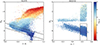 |
Fig. 1 Colour-magnitude diagrams of the whole RAVE and SEGUE G-dwarf data from 2MASS and SDSS photometry, respectively.The applied cuts are shown in black lines. |
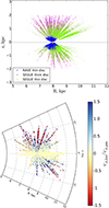 |
Fig. 2 Spatial distribution of the RAVE and SEGUE samples. Top panel: Galactic cylindrical coordinates R and z of thefinal SEGUE (both thin and thick disc stars) and RAVE data samples (only thin disc stars). The position of the Sun at Galactocentric distance R0 = 8 kpc and height z = 0 kpc is marked with a yellow circle. Bottom panel: whole SEGUE sample projected on the Galactic plane. The value of ϕ = 0° corresponds to the Sun-Galactic centre axis. |
3 Jeans analysis
In this section we discuss the properties of the asymmetric drift, when applied to a large volume in Galactocentric distance R and height above the Galactic midplane z. The equation that we are going to formulate here is the basis of our work.
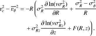
The asymmetric drift is defined as the lag in tangential speed of tracer populations with respect to the rotation curve, 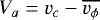 . The exact value of this quantity depends on stellar population properties and varies with the position in the Galaxy. This implies that in order to convert mean tangential velocities
  to the rotation curve, we need to correct them for V a. To quantify the asymmetric drift we use the same notation as in Golubov et al. (2013) and start with the radial Jeans equation for a stationary and axisymmetric system (in cylindrical coordinates and with negligible mean radial and vertical motion):
 (1)
(1)
Here ν and  are the tracer density and velocity ellipsoid,
  is the mean tangential speed of the population, vc is its circular speed defined in the midplane and F(R, z) measures the vertical variation of the radial force, that is,
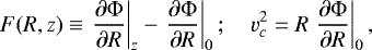 (2)
(2)
where Φ is the total gravitational potential. The right-hand side of Eq. (1) is a measure of the asymmetric drift we are interested in. The last term vanishes at z = 0, but it should not be neglected at z≠0. Indeed, as with the increase of height above the midplane, the radial gradient of the Galactic gravitational potential decreases, as does the measured tangential speed. This effect, if not taken into account, can result in two biases. Firstly, the derived circular velocity can be underestimated by a few killometers per second, causing a shift of the rotation curve as a whole. Secondly, the typical distance of stars from the midplane varies at different Galactocentric radii due to the sample geometry (see SEGUE sample in Fig. 2). This can cause a distortion of the rotation curve, which is unacceptable as the robust reconstruction of the shape of the local rotation curve is the very aim of this work. The penultimate term is the well-known tilt term, which does not vanish in general even in the midplane (see Eq. (4) below). Since these vertical correction terms lead to a systematic variation of the asymmetric drift increasing with |z|, we take them into account throughout this work, even for the relatively local RAVE sample with the range of useful distances limited to ±0.5 kpc from the Sun (Fig. 2, top panel). The details of the derivation and the assumptions made are provided in Appendix A. Here we explain only the essential part of our treatment of Eq. (1).
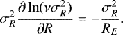
The rotation curve, which we wish to determine, depends on the same Galactic potential. Therefore, we need to check carefully that we are not biasing the result implicitly by adopting a special model for the potential, entering Eq. (1) through the vertical gradients of tracer density and the radial force. We use a five-component model of the Galaxy with a spherical Navarro–Frenk–White (NFW) Dark Matter (DM) halo (Navarro et al. 1995) with a local density ρh⊙ and power law slope γh = −1, a bulge component with mass Mb and three exponential discs for the gas, and the thin and thick disc with local surface densities Σi and radial and vertical scale lengths Ri and hi. The gaseous disc has an inner hole with a radius of Rcut,g = 4 kpc. The values of all used parameters are given in Table 1. With this Galactic model we calculate the exact value of the vertical variation of the radial force using the GalPot code1 (a stand-alone version of Walter Dehnen’s GalaxyPotential C++ code, Dehnen & Binney 1998a).
In the tilt term in Eq. (1) we parametrize  as
as
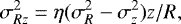 (3)
(3)
where the parameter η describes the orientation of the velocity ellipsoid relative to the direction of the Galactic centre. The logarithmic derivative of 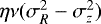 can be further parametrized with some characteristic scale height hνσ (which describes the vertical variation of the tracer density and velocity ellipsoid orientation and is in general a function of R and z), leading to
![Mathematical equation: \begin{equation*} \sigma_{Rz}^2 \frac{\partial \ln (\nu \sigma_{Rz}^2)}{\partial z} = \eta \frac{\sigma_R^2 - \sigma_z^2}{R}\left[ 1 - \frac{z}{h_{\nu \sigma}}\right].\end{equation*}](/articles/aa/full_html/2018/06/aa31143-17/aa31143-17-eq10.png) (4)
(4)
The first term in Eq. (1) can be characterized by the radial scale length RE (which again may depend on R and z), and therefore reads
 (5)
(5)
At this point we note that under the assumption of a constant disc thickness and a constant shape of the velocity ellipsoid  , which implies
  , we find RE related to the radial scale length of thetracer density ν through Rν = 2 RE = const. We use this assumption below in order to convert the measured RE into the radial scale lengths of the subpopulations (see Sect. 4).
Finally, we can write the Jeans equation (Eq. (1)) as
 (6)
(6)
This equation is still equivalent to Eq. (1). With a specification of the parameters/functions F(R, z), η, hνσ, RE (e.g. RE independent of R, z) we lose generality.
Properties of the Galaxy used for calculations.
4 Solar motion and radial scale lengths
Before using the mean measured relative velocities of the tracer stars to find the mean tangential velocities  and correct them for the asymmetric drift, we need to correct for the peculiar motion of the Sun
  , that is, to convert the velocities to the local standard of rest. The determination of U⊙ and W⊙ from the stellar kinematics in the solar neighbourhood is not a matter of difficulty. For the radial and verticalcomponents of the solar motion we adopt the values from Schönrich et al. (2010): U⊙ = 11.1 km s−1, W⊙= 7.25 km s−1, which are also consistent with our data sets. In contrast, the determination of the tangential component V ⊙ is challenging. Due to the fact that the observed tangential motion of stellar populations is affected both by the solar peculiar velocity and the asymmetric drift, the task of disentangling them poses a problem. The classical value based on hipparcos data is V ⊙ = 5.2 km s−1 (Dehnen & Binney 1998b). The more recent and widely used ones lie between approximately 10 and 12 km s−1 (e.g. 12.24 ± 0.47 km s−1 in Schönrich et al. 2010). However, among recent estimates there are also values as high as ~24 km s−1 (Bovy et al. 2012b) indicating that the local stellar motions could also be influenced by non-axisymmetric Galactic features such as spiral arms (Siebert et al. 2012; Monari et al. 2016) and a bar (Dehnen 2000; Monari et al. 2017; Pérez-Villegas et al. 2017). At the lower limit, there is V ⊙ = 3.06 ± 0.68 km s−1 found by uspreviously in Golubov et al. (2013). Rather than taking an old value of V ⊙ together with the radial scale lengths for three metallicity populations, we re-determine them here in order to quantify the impact of our improved analysis in combination with the new distances and improved proper motions. To find the tangential component V ⊙ we apply the new Strömberg relation, as in Golubov et al. (2013), to the local RAVE data, but now including the vertical correction terms discussed in the previous section. We assume a Galactocentric distance of the Sun of R0 = 8 kpc, which is consistent with Reid (1993) as well as with a more recent study by Gillessen et al. (2009). Then adopting the proper motion of Sgr A* from Reid & Brunthaler (2005) we get the solar Galactocentric velocity v⊙ = 241.6 ± 15 km s−1.
Applying Eq. (6) at R = R0 and using v0:= vc(R0) = v⊙− V ⊙ and  , we write for the left-hand side:
 (7)
(7)
This leads to the new version of the Strömberg relation:
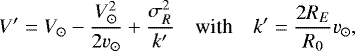 (8)
(8)
and the generalized version of V ′:
![Mathematical equation: \begin{align*} & V^{\prime}:={{\Delta}} V\\ &\quad\quad\,\, +\frac{\sigma_R^2 -\sigma_{\phi}^2 +R_0 F(R_0,z) + \eta (\sigma_R^2 - \sigma_z^2)\left[ 1 - \frac{z}{h_{\nu\sigma}}\right] -{{\Delta}} V^2}{2 v_{\odot}}.\nonumber \end{align*}](/articles/aa/full_html/2018/06/aa31143-17/aa31143-17-eq20.png) (9)
(9)
To make practical use of Eqs. (8) and (9), that is, to determine values of V ⊙ and RE, we need to bin our data sample into sub-bins with different kinematics. For this purpose we separate the RAVE sample into three subpopulations with different metallicities and then bin each subpopulation in (J–K) colour. The top panel of Fig. 3 shows such a binning of the squared radial velocity dispersion  and measured velocity ΔV, which can be calculated straightforwardly, without knowledge of V ⊙. One can clearly see that the kinematic properties change systematically with both metallicity and colour. Using the same binning we plot V ′ versus
  (Fig. 3, bottom panel). For simplicity, we assume here that η = const. = 0.8 as derived in Binney et al. (2014) from the RAVE data. We also treat hνσ as independent of colour, though differing with metallicity and select appropriate values from the disc model of Just & Jahreiß (2010; see Appendix A). The height above the midplane z in Eq. (9) is calculated for each metallicity-colour bin as a mean value of the absolute z for individual stars.
As in Golubov et al. (2013) we still see the systematic difference of  between metallicity bins, but the linear dependencies show a larger scatter. The assumption that RE, similar to hνσ, is approximately the same for all colours inside a given metallicity bin, but differs with metallicity, allows us to derive RE values for the three metallicity subpopulations as well as V ⊙. To do so we perform a simultaneous linear fit of the metallicity-colour sequences (shown with colour-coded dashed lines in Fig. 3, bottom panel). The inverse slopes of the fitting lines
  can be directly converted to RE,i, which under the assumption of constancy of the disc thickness and the shape of velocity ellipsoid (see Sect. 3) gives us the radial scale lengths for the selected populations. The solar peculiar motion can be readout from the V ′ extrapolated to zero radial velocity dispersion:
The updated value of the tangential component of the solar peculiar motion is found to be V ⊙ = 4.47 ± 0.8 km s−1, which translates to the local circular velocity v0 ≈ 237 ± 16 km s−1. The radial scale lengths for the metallicity bins are Rd (0 < [Fe/H] < 0.2) = 2.07 ± 0.2 kpc, Rd (−0.2 < [Fe/H] < 0) = 2.28 ± 0.26 kpc and Rd (−0.5 < [Fe/H] <−0.2) = 3.05 ± 0.43 kpc, which together with V ⊙ is in agreement with our old values from Golubov et al. (2013).
Now we must check whether SEGUE stars also follow the same trend. For this purpose we split the thin disc SEGUE sample into the same metallicity bins and consider only stars with Galactocentric distances 7.5 < R < 8.5 kpc. The subdivision in colours is not possible for this data set because of its narrow colour range. Another characteristic of this sample is that G-dwarfs are distributed over a significantly larger range of |z| (Fig. 2, top). Furthermore, although we do not reconstruct here the shape and orientation of the velocity ellipsoid as a function of R and z, we may roughly account for the vertical gradients of  and
and  . To do so we apply Eq. (9) for the calculation of V ′, not to the whole metallicity bin, but separately in vertical sub-bins (|z| = 0 ... 1.5 kpc with a step of 0.5 kpc) and calculate the resultingV ′ by taking a weighted mean of the valuesobtained for different |z|.
The SEGUE points (filled circles in Fig. 3, bottom panel) demonstrate good consistency with the RAVE data, which means that for further analysis of the SEGUE thin disc sample we can securely use the values of scale lengths derived from RAVE. This is an important result, accounting for all uncertainties of the metallicity calibration in RAVE and possible velocity biases for SEGUE. To be even more precise we can inverse the problem and read out scale lengths for individual points adopting the solar peculiar velocity derived with the RAVE data. The values of Rd calculated for the SEGUE data in such a way (see the three solid black lines in Fig. 3, bottom panel) are: Rd (0 < [Fe/H] < 0.2) = 1.91 ± 0.23 kpc, Rd (−0.2 < [Fe/H] < 0) = 2.51 ± 0.25 kpc, and Rd (−0.5 < [Fe/H] <−0.2) = 3.55 ± 0.42 kpc. We use these new values and V ⊙ = 4.47 ± 0.8 km s−1 in our further analysis.
The linearity of the asymmetric drift correction, that is, constancy of Rd versus  , is still under debate. Nevertheless, even if the asymmetric drift dependence on
  in fact turns out to be non-linear for small
  (as assumed by Schönrich et al. 2010), it will correspond to some shift in the measured circular velocity. We do not, however, expect this shift to change drastically at different Galactocentric radii. To the first approximation this would produce only a parallel displacement of the measured rotation curve. Being interested in the general shape of the rotation curve, not in the exact value of the rotation velocity, we apply the solar velocity and the radial scale lengths derived by Eq. (8) at all Galactocentric radii.
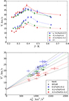 |
Fig. 3 Recalculation and consistency check of the asymmetric drift correction for the RAVE and local SEGUE data samples. The RAVE data are recalculated using the improved distances from McMillan et al. (2018) and UCAC5 proper motions. Top panel: σR and ΔV as functionsof (J–K) 2MASS colour for different metallicity bins (compare to Fig. 2 in Golubov et al. 2013). Bottom panel: V ′ as a functionof |

5 Asymmetric drift and rotation curve
Now, with updated values for the solar peculiar velocity and the radial scale lengths for three populations of the selected metallicities, we proceed to the determination of the rotation curve in the extended solar neighbourhood. We go back to the Jeans equation formulated for arbitrary (R, z) (see Eq. (6)) and apply it to the thin disc SEGUE stars. In principle, Eq. (6) can be directly used for the determination of the rotation velocity as all terms on the right-hand side are now known and the mean tangential speed can be expressed as  , where v⊙ is the tangential speed of the Sun and (−ΔV) is the mean observed tangential velocity with respect to the Sun. However, we would prefer to formulate the expression of the rotation velocity in terms of the asymmetric drift V a, so we recall its definition:
 (11)
(11)
Inserting 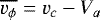 into the left-hand side of Eq. (6), we arrive at the quadratic equation for the asymmetric drift:
![Mathematical equation: \begin{eqnarray*} && V_a^2 -2 v_c V_a - R \Bigg( F(R,z)\\ && \quad\quad + \eta \frac{\sigma_R^2 - \sigma_z^2}{R}\left[ 1 - \frac{z}{h_{\nu \sigma}}\right]- \frac{\sigma_R^2}{R_E}+ \frac{\sigma_R^2 -\sigma_{\phi}^2}{R}\Bigg ) = 0. \nonumber \end{eqnarray*}](/articles/aa/full_html/2018/06/aa31143-17/aa31143-17-eq34.png) (12)
(12)
We solve Eq. (12) with respect to V a and get:
![Mathematical equation: \begin{eqnarray*} V_a &=& v_c(R) - \Bigg\{ v_c^2(R) + R \bigg( F(R,z) \phantom{\bigg(}\\ && \phantom{\bigg(} +\,\eta \frac{\sigma_R^2 - \sigma_z^2}{R}\left[ 1 - \frac{z}{h_{\nu \sigma}}\right] - \frac{\sigma_R^2}{R_E} + \frac{\sigma_R^2 -\sigma_{\phi}^2}{R} \bigg) \Bigg\}^{1/2} \nonumber\\ &\approx & \frac{-R F(R,z) - \eta (\sigma_R^2 - \sigma_z^2)\left[ 1 - \frac{z}{h_{\nu \sigma}}\right] + \sigma_R^2\frac{R}{R_E} - (\sigma_R^2 -\sigma_{\phi}^2)}{2v_c(R)}, \end{eqnarray*}](/articles/aa/full_html/2018/06/aa31143-17/aa31143-17-eq35.png) (13)
(13)
where the last line corresponds to the linear approximation ignoring the  term. The difference of the non-linear and linear values for V a is of the order of 5% or 1 km s−1.
The final formula for calculating the rotation velocity at radius R for each bin (R, z) is from Eq. (11);
 (14)
(14)
with the asymmetric drift correction V a given by Eq. (13). As V a is itself a function of vc(R), the determination of the rotation velocity is an iterative procedure, during which we assume vc ∝ Rα. We start with some small α as initial value. At each step of the iteration, the reconstructed rotation curve is fitted and the new value of α is derived to be plugged back into Eq. (13) via vc(R). The iteration procedure converges very quickly, after two or three cycles.
We bin thin disc SEGUE stars, again separated into three metallicities as before, in Galactocentric distances with equal step of 0.4 kpc. The further data analysis is not the same for all distance bins. As mentioned above, the SEGUE stars are in general distributed over a large range in |z|, so we would like to take into account the vertical gradients in  and
and  by applying our equations separately at different heights for each distance. As one can see from the top panel of Fig. 2, such |z|-binning for the thin disc sample is justified only close to R0, approximately for 7 kpc < R < 9 kpc, because at larger Galactocentric distances the majority of stars are located at approximately the same height, such that low-|z| bins would be essentially empty and suffering from high Poisson noise. For this reason we do not bin in |z| outside this distance range. Taking this into account, at R < 7 kpc and R > 9 kpc for each R-bin we find the mean tangential velocity
  (dashed colour-coded lines in Fig. 4), as well as three velocity dispersions and mean values of R and |z|. Then we apply the correction for the asymmetric drift from Eq. (13), which is typically ~20 km s−1. For 7 kpc < R < 9 kpc we do the same, but separately for three vertical bins (as before, |z| = 0 ... 1.5 kpc with a step of 0.5 kpc), and then calculate the weighted mean vc at each R. The obtained rotation curves representing different metallicity bins are shown as solid lines in Fig. 4 and are broadly consistent with each other within the error bars.
Between 8 and 10 kpc the rotation curve is flat to an accuracy of a few kilometres per second, and definitely does not show the 10 km s−1 dip described by Sofue et al. (2009, 2010). On the other hand, the inner part of our rotation curve demonstrates a metallicity-dependent rise with the amplitude up to 10 km s−1, similar to the one attested by Sofue et al. (2009, 2010).
We perform a power-law fit V c ∝ Rα simultaneously to all three rotation curves and find a small power law index α = 0.033 ± 0.034 (fit shown in Fig. 4 with a dashed line). This transforms into the local slope of the rotation curve d V c ∕dR = 0.98 ± 1 km s−1 kpc−1. However, the existing measurements of the Oort constants point to a moderately negative slope: the classical value from Binney & Tremaine (2008) is dV c ∕dR = −2.4 ± 1 km s−1 kpc−1, while the more recent study by Bovy (2017) from TGAS data suggests an even steeper slope of − 3.4 ± 0.6 km s−1 kpc−1. Still, we must keep in mind that the Oort constants measure only a very local slope of the rotation curve, which may be more strongly perturbed by the local spiral arm structure and the bar, while our analysis goes all the way to 1–2 kpc away from the Sun.
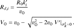
The thick disc SEGUE stars are not very instrumental in reconstructing the rotation curve, as the radial scale length of the thick disc is poorly constrained. We can solve the inverse problem by using the data to reconstruct the radial scale length of the thick disc assuming the rotation curve already known. We express Rd from Eq. (8) and calculate it for ten metallicity bins of the thick disc. For the parameter hνσ of the thick disc we use a value of 800 pc, similar to its scale height (Just et al. 2011). Furthermore, we take only the local thick disc sample with 7.5 kpc < R < 8.5 kpc in order to avoid regions where our results can be biased by the uncertainty in the vertical correction term (this effect is not so important for the thin disc sample, as its stars are in general located at smaller |z| than those of the thick disc). The resulting Rd is shown in Fig. 5 with red points. Though the data points show some small variation of Rd with [Fe/H], the constant value of the scale length 2.1 ± 0.05 kpc is more robust (see the darker one-sigma area in Fig. 5). In other words, the chemically defined thick disc behaves as a single kinematically homogeneous population. The value of the thick disc scale length found here is consistent with simulations by Minchev et al. (2015) and with the data analysis by Bovy et al. (2012b) and Kordopatis et al. (2017). When binning the local SEGUE thick disc sample in metallicity, we calculate Rd for the “effective” quantities in the bin: velocity dispersions are determined for all stars and also mean |z| and R. Such “effective” values are representative in the cases of R and velocity dispersions because our data are very local in terms of Galactocentric distances and are expected to be kinematically homogeneous, so the velocity dispersions should not have a strong gradient in vertical direction. On the other hand, the mean value of |z| might be misleading as the vertical distribution of stars is inhomogeneous. The vertical correction and the tilt term in V ′ (Eq. (9)) are quite sensitive to z, so to cross-check our results we apply Eq. (8) for 4 |z|-bins (0 to 2 kpc with a 0.5 kpc step) with no binning in metallicity as the data are not abundant enough to allow a simultaneous separation in both |z| and [Fe/H]. The resulting scale length, which is calculated again as a weighted mean of the values found for different |z|, deviates only slightly from the value found at the previous step: Rd = 2.05 ± 0.22 kpc. We overplot it in Fig. 5 with a blue dot for the mean metallicity of the local thick disc sample. A good agreement between the values of scale length calculated via the different binning of our sample in the parameter space ensures us of the robustness of the derived result.
 |
Fig. 4 Rotation curve in the extended solar neighbourhood traced via SEGUE stars. The thin disc stars are split into the same three metallicity bins as in Sect. 4. For each distance bin the mean rotation velocity |
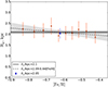 |
Fig. 5 Radial scale length Rd of the thick disc versus metallicity. Considered are SEGUE thick disc stars with 7.5 kpc < R < 8.5 kpc, 4195 in total. Red points show the radial scale lengths calculated for each metallicity bin with the “effective” quantities in Eq. (9). The points are fitted with a constant and also with Rd linearly dependent on [Fe/H] (solid and dashed lines). One-sigma areas are shown in grey. The blue point corresponds to the value of scale length derived in case of binning the same sample in 4 |z|-bins. |
6 Discussion and conclusions
In this paper we performed the revision and improvement of the methods developed previously in Golubov et al. (2013). Starting from the classical Jeans analysis we arrived at the new Strömberg relation for the asymmetric drift and applied it locally to the most recent RAVE data. This enabled us to update the value of the solar peculiar motion to V ⊙ = 4.47 ± 0.8 km s−1. This is lower than the typical values reported by other authors, which are around 10–12 km s−1. However, in the study of Sharma et al. (2014) also based on the RAVE data, though in the framework of a different Galaxy model, the solar peculiar velocity is smaller as well:  km s−1. We also found radial scale lengths for the three metallicity populations, which are Rd (0 < [Fe/H] < 0.2) = 2.07 ± 0.2 kpc, Rd (−0.2 < [Fe/H] < 0) = 2.28 ± 0.26 kpc, and Rd (−0.5 < [Fe/H] <−0.2) = 3.05 ± 0.43 kpc. Our analysis demonstrates good consistency of the SEGUE and the RAVE data in terms of kinematics. With the peculiar velocity of the Sun derived from the RAVE sample, SEGUE data give similar values for the scale lengths: Rd (0 < [Fe/H] < 0.2) = 1.91 ± 0.23 kpc, Rd (−0.2 < [Fe/H] < 0) = 2.51 ± 0.25 kpc, and Rd (−0.5 < [Fe/H] <−0.2) = 3.55 ± 0.42 kpc.
Subsequently, we used the SEGUE sample of the thin disc G-dwarfs to reconstruct the rotation curve of the Milky Way, ranging from 7 to 10 kpc in Galactocentric radius. We took into account the asymmetric drift correction (Eq. (13)) and showed that the resulting rotation curve is essentially flat (Fig. 4). Thus, the existence of any features in the rotation curve just outside the solar radius is discarded in the framework of our analysis. The formal power-law fit to the rotation curve implies a positive slope α =0.033 ± 0.034 consistent with a flat rotation curve, although we see that its local value is probably smaller. The corresponding radial gradient of the circular speed is d V c ∕dR = 0.98 ± 1 km s−1 kpc−1, which is in agreement with the findings of Sharma et al. (2014), who derived a similar value from the RAVE data: 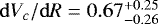 km s−1 kpc−1.
Using SEGUE data and relying on the determined slope of the rotation curve, we also calculated the radial scale length of the thick disc: 2.05 ± 0.22 kpc. No strong dependence on metallicity was observed. Values of the quantities derived in this paper are summarized in Table 2.
Finally, we must discuss the dependence of our results on the assumed constants and parameters. The pair (R0,v⊙), on the one hand, influences the derived stellar spatial distribution and velocities from the observables. On the other hand, it enters the equation for the asymmetric drift correction (see Eq. (13)). For the recommended values from Bland-Hawthorn & Gerhard (2016) (R0,v⊙) = (8.2 kpc, 248 km s−1) the change in the re-calculated solar peculiar velocity and scale heights for the three metallicity bins lie well within one sigma and the changes in the rotation curve can be mostly described in terms of a vertical shift to higher velocities and horizontal translation to larger Galactocentric distances; a slope of α =0.024 ± 0.031 is found, which is again consistent with a flat rotation curve.
What is the impact of the solar peculiar motion? Changes of  add quadratically to the corresponding velocity dispersions. The vertical velocity has no other impact on the result, but we should check that the vertical component of the mean measured relative velocity of the stars in the sample is approximately − W⊙, which is indeed the case. U⊙ enters the velocity transformations to cylindrical coordinates, so every time we change V ⊙, R0 or v⊙, we have to adapt it to have
  as we assumed in Sect. 3. However, this correction is small and we can neglect it as it is surely beyond the accuracy we can hope to achieve in the framework of our approach. V ⊙ has a largerimpact on the results as the asymmetric drift correction depends on it, mainly via vc and the scale lengths (see Eq. (13)). We test two values of V ⊙, ~3 km s−1 (Golubov et al. 2013) and ~7.6 km s−1 (Sharma et al. 2014). The rotation curve slope is then α = 0.039 ± 0.034 and α = 0.014 ± 0.028, respectively.We also test the sensitivity of our results to the vertical scale heights hνσ as they are not tightly constrained. Changing hνσ by ± 20% leads to slopes of α = 0.022 ± 0.03 and α =0.049 ± 0.038, which deviate from our standard value by less than 0.5σ.
To quantify the vertical gradient of the radial force term we assume a Galaxy model, that is, we use some form of the potential as an input. However, we believe that the rotation curve obtained in Sect. 5 is not strongly predefined by this choice. The RF(R, z) term is not a dominating one in the asymmetric drift correction, so with respect to the rotation velocity, it is a first-order correction. The modification of the potential will enter vc as a second-order correction only, and this already meets the limit of our accuracy. As we inferred by running the tests with the GalPot code, the main contribution to the vertical correction of the radial force comes from the thin disc, thus its scale length and scale height are the main sources of uncertainty in this term. Taking a Rd value of 2 or 3 kpc we arrive at a rotation curve that is correspondingly slightly steeper (α = 0.041 ± 0.041) or flatter (α = 0.027 ± 0.029) than the one we presented in Fig. 4. Testing hz of 200 and 400 pc results in similar changes: α = 0.041 ± 0.036 and α = 0.026 ± 0.03. The impact of varying Rd and hz of the other discs is negligible.
None of these deviations from our main result produce essential changes in the derived rotation curve shape. We therefore conclude that, in the framework of the developed analysis, our outcome is robust with respect to the small changes of our constants and the pre-choice of the Galactic potential. Our analysis of the local rotation curve does not support the existence of any special features in its shape, such as a significant dip at R = 9 kpc.
Summary of the results.
Acknowledgements
This work was supported by Sonderforschungsbereich SFB 881 “The Milky Way System” (subprojects A6 and A5) of the German Research Foundation (DFG). Funding for RAVE has been provided by: the Australian Astronomical Observatory; the Leibniz-Institut fuer Astrophysik Potsdam (AIP); the Australian National University; the Australian Research Council; the French National Research Agency; the German Research Foundation (SPP 1177 and SFB 881); the European Research Council (ERC-StG 240271 Galactica); the Istituto Nazionale di Astrofisica at Padova; The Johns Hopkins University; the National Science Foundation of the USA (AST-0908326); the W. M. Keck foundation; the Macquarie University; the Netherlands Research School for Astronomy; the Natural Sciences and Engineering Research Council of Canada; the Slovenian Research Agency (P1-0188); the Swiss National Science Foundation; the Science & Technology Facilities Council of the UK; Opticon; Strasbourg Observatory; and the Universities of Groningen, Heidelberg and Sydney. The RAVE web site is at https://www.rave-survey.org. Funding for SDSS-I and SDSS-II has been provided by the Alfred P. Sloan Foundation, the Participating Institutions, the National Science Foundation, the U.S. Department of Energy, the National Aeronautics and Space Administration, the Japanese Monbukagakusho, the Max Planck Society, and the Higher Education Funding Council for England. The SDSS Web Site is http://www.sdss.org. UCAC5 proper motions and the distances from McMillan et al. (2018) were obtained with the use of the European Space Agency (ESA) mission Gaia (https://www.cosmos.esa.int/gaia), processed by the Gaia Data Processing and Analysis Consortium (DPAC, https://www.cosmos.esa.int/web/gaia/dpac/consortium). Funding for the DPAC has been provided by national institutions, in particular the institutions participating in the Gaia Multilateral Agreement. The authors are very grateful to Young-Sun Lee and Timothy C. Beers for providing their SEGUE data sample for our analysis and for fruitful discussions. We also thank the anonymous referee for the detailed suggestions, which improved the paper significantly.
Appendix A Vertical gradient of tracer populations
The tilt term in Eq. (1) describes the vertical density gradient and the change in the tilt of the velocity ellipsoid. The tilt angle of the velocity ellipsoid is defined as
 (A.1)
(A.1)
On the other side, the tilt angle can be parametrized with a parameter η, which describes the orientation of the velocity ellipsoid relative to the Galactic centre
 (A.2)
(A.2)
Assuming that αtilt is small, one then arrives at the following relation for  :
:
 (A.3)
(A.3)
The derivative of  is
is
![Mathematical equation: \begin{align*} &\frac{\partial \sigma_{Rz}^2}{\partial z} = \frac{\eta}{R}(\sigma_R^2-\sigma_z^2) - \frac{z}{R}(\sigma_R^2-\sigma_z^2)\frac{\partial \eta}{\partial z}\\ &\quad\quad\quad\,\,+\eta \frac{z}{R} \left(\frac{\partial \sigma_R^2}{\partial z} - \frac{\partial \sigma_z^2}{\partial z}\right) = \sigma_{Rz}^2 \left[ \frac{1}{z} + \frac{\partial \ln \eta}{\partial z} + \frac{\partial \ln(\sigma_R^2-\sigma_z^2)}{\partial z} \right]. \nonumber \end{align*}](/articles/aa/full_html/2018/06/aa31143-17/aa31143-17-eq50.png) (A.4)
(A.4)
Thus, the tilt term in Eq. (1) together with Eq. (A.4) gives
![Mathematical equation: \begin{equation*} \sigma_{Rz}^2 \left[ \frac{1}{z} + \frac{\partial \ln(\eta\nu (\sigma_R^2-\sigma_z^2))}{\partial z} \right].\end{equation*}](/articles/aa/full_html/2018/06/aa31143-17/aa31143-17-eq51.png) (A.5)
(A.5)
The second term in the brackets can be parametrized with some characteristic scale height hνσ, so we arrive at
![Mathematical equation: \begin{align*} &\sigma_{Rz}^2 \frac{\partial \ln (\nu \sigma_{Rz}^2)}{\partial z} = \frac{\sigma_{Rz}^2}{z} \left[ 1 - \frac{z}{h_{\nu \sigma}}\right] \nonumber\\ & \quad\quad\quad\quad\quad\,\,\,\,= \eta \frac{\sigma_R^2 - \sigma_z^2}{R}\left[ 1 - \frac{z}{h_{\nu \sigma}}\right].\end{align*}](/articles/aa/full_html/2018/06/aa31143-17/aa31143-17-eq52.png) (A.6)
(A.6)
We expect that the vertical variation of η and of  is small compared to the gradient of the tracer density ν. We can therefore relate the scale height hνσ to the characteristic scale height of the tracer density. For this purpose we use the half-thickness values of the mono-age subpopulations with ages of 4, 6, and 10 Gyr, taken from the local thin disc model (Just & Jahreiß 2010). The youngest subpopulation represents the bin with the highest metallicity. The adopted values of hνσ are 360, 430, and 530 pc, respectively.
References
- Binney, J., & Tremaine, S. 2008, Galactic Dynamics (Princeton: Princeton Univ. Press) [Google Scholar]
- Binney, J., Burnett, B., Kordopatis, G., et al. 2014, MNRAS, 439, 1231 [NASA ADS] [CrossRef] [Google Scholar]
- Bland-Hawthorn, J., & Gerhard, O. 2016, ARA&A, 54, 529 [NASA ADS] [CrossRef] [EDP Sciences] [Google Scholar]
- Bovy, J. 2017, MNRAS, 468, L63 [NASA ADS] [CrossRef] [Google Scholar]
- Bovy, J., Allende Prieto, C., Beers, T. C., et al. 2012a, ApJ, 759, 131 [NASA ADS] [CrossRef] [Google Scholar]
- Bovy, J., Rix, H.-W., Liu, C., et al. 2012b, ApJ, 753, 148 [NASA ADS] [CrossRef] [Google Scholar]
- Chemin, L., Renaud, F., & Soubiran, C. 2015, A&A, 578, A14 [NASA ADS] [CrossRef] [EDP Sciences] [Google Scholar]
- Chemin, L., Huré, J.-M., Soubiran, C., et al. 2016, A&A, 588, A48 [NASA ADS] [CrossRef] [EDP Sciences] [Google Scholar]
- Cheng, J. Y., Rockosi, C. M., Morrison, H. L., et al. 2012, ApJ, 752, 51 [NASA ADS] [CrossRef] [Google Scholar]
- Dehnen, W. 2000, AJ, 119, 800 [NASA ADS] [CrossRef] [Google Scholar]
- Dehnen, W., & Binney, J. 1998a, MNRAS, 294, 429 [NASA ADS] [CrossRef] [Google Scholar]
- Dehnen, W., & Binney, J. 1998b, MNRAS, 298, 387 [NASA ADS] [CrossRef] [Google Scholar]
- Eisenstein, D. J., Weinberg, D. H., Agol, E., et al. 2011, AJ, 142, 72 [Google Scholar]
- Gaia Collaboration (Brown, A. G. A., et al.), 2016, A&A, 595, A2 [NASA ADS] [CrossRef] [EDP Sciences] [Google Scholar]
- Gillessen, S., Eisenhauer, F., Fritz, T. K., et al. 2009, ApJ, 707, L114 [NASA ADS] [CrossRef] [Google Scholar]
- Golubov, O., Just, A., Bienaymé, O., et al. 2013, A&A, 557, A92 [NASA ADS] [CrossRef] [EDP Sciences] [Google Scholar]
- Huang, Y., Liu, X.-W., Yuan, H.-B., et al. 2016, MNRAS, 463, 2623 [NASA ADS] [CrossRef] [Google Scholar]
- Just, A., & Jahreiß, H. 2010, MNRAS, 402, 461 [NASA ADS] [CrossRef] [Google Scholar]
- Just, A., Gao, S., & Vidrih, S. 2011, MNRAS, 411, 2586 [NASA ADS] [CrossRef] [Google Scholar]
- Kafle, P. R., Sharma, S., Lewis, G. F., & Bland-Hawthorn, J. 2012, ApJ, 761, 98 [NASA ADS] [CrossRef] [Google Scholar]
- Kordopatis, G., Wyse, R. F. G., Chiappini, C., et al. 2017, MNRAS, 467, 469 [NASA ADS] [Google Scholar]
- Kunder, A., Kordopatis, G., Steinmetz, M., et al. 2017, AJ, 153, 75 [NASA ADS] [CrossRef] [Google Scholar]
- Lee, Y. S., Beers, T. C., An, D., et al. 2011, ApJ, 738, 187 [NASA ADS] [CrossRef] [Google Scholar]
- Liu, X.-W., Yuan, H.-B., Huo, Z.-Y., et al. 2014, in Setting the Scene for Gaia and LAMOST, eds. S. Feltzing, G. Zhao, N. A. Walton, & P. Whitelock, IAU Symp., 298, 310 [NASA ADS] [Google Scholar]
- López-Corredoira, M. 2014, A&A, 563, A128 [NASA ADS] [CrossRef] [EDP Sciences] [Google Scholar]
- McMillan, P. J., Kordopatis, G., Kunder, A., et al. 2018, MNRAS, in press, [arXiv:1707.04554] [Google Scholar]
- Minchev, I., Martig, M., Streich, D., et al. 2015, ApJ, 804, L9 [NASA ADS] [CrossRef] [Google Scholar]
- Monari, G., Famaey, B., & Siebert, A. 2016, MNRAS, 457, 2569 [NASA ADS] [CrossRef] [Google Scholar]
- Monari, G., Kawata, D., Hunt, J. A. S., & Famaey, B. 2017, MNRAS, 466, L113 [NASA ADS] [CrossRef] [Google Scholar]
- Navarro, J. F., Frenk, C. S., & White, S. D. M. 1995, MNRAS, 275, 720 [NASA ADS] [CrossRef] [Google Scholar]
- Pérez-Villegas, A., Portail, M., Wegg, C., & Gerhard, O. 2017, ApJ, 840, L2 [NASA ADS] [CrossRef] [Google Scholar]
- Reid, M. J. 1993, ARA&A, 31, 345 [NASA ADS] [CrossRef] [Google Scholar]
- Reid, M. J., & Brunthaler, A. 2005, in Future Directions in High Resolution Astronomy, eds. J. Romney & M. Reid, ASP Conf. Ser., 340, 253 [NASA ADS] [Google Scholar]
- Reid, M. J., Menten, K. M., Brunthaler, A., et al. 2014, ApJ, 783, 130 [Google Scholar]
- Robin, A. C., Reylé, C., Derrière, S., & Picaud, S. 2003, A&A, 409, 523 [NASA ADS] [CrossRef] [EDP Sciences] [Google Scholar]
- Schönrich, R., Binney, J., & Dehnen, W. 2010, MNRAS, 403, 1829 [NASA ADS] [CrossRef] [Google Scholar]
- Sharma, S., Bland-Hawthorn, J., Binney, J., et al. 2014, ApJ, 793, 51 [NASA ADS] [CrossRef] [Google Scholar]
- Siebert, A., Famaey, B., Binney, J., et al. 2012, MNRAS, 425, 2335 [NASA ADS] [CrossRef] [Google Scholar]
- Skrutskie, M. F., Cutri, R. M., Stiening, R., et al. 2006, AJ, 131, 1163 [NASA ADS] [CrossRef] [Google Scholar]
- Sofue, Y., Honma, M., & Omodaka, T. 2009, PASJ, 61, 227 [NASA ADS] [Google Scholar]
- Sofue, Y., Honma, M., & Omodaka, T. 2010, PASJ, 62, 1367 [NASA ADS] [CrossRef] [Google Scholar]
- Steinmetz, M., Zwitter, T., Siebert, A., et al. 2006, AJ, 132, 1645 [NASA ADS] [CrossRef] [Google Scholar]
- Wegg, C., Gerhard, O., & Portail, M. 2015, MNRAS, 450, 4050 [NASA ADS] [CrossRef] [Google Scholar]
- Wojno, J., Kordopatis, G., Steinmetz, M., et al. 2016, MNRAS, 461, 4246 [NASA ADS] [CrossRef] [Google Scholar]
- Wojno, J., Kordopatis, G., Piffl, T., et al. 2017, MNRAS, 468, 3368 [NASA ADS] [CrossRef] [Google Scholar]
- Yanny, B., Rockosi, C., Newberg, H. J., et al. 2009, AJ, 137, 4377 [NASA ADS] [CrossRef] [Google Scholar]
- Zacharias, N., Finch, C., & Frouard, J. 2017, AJ, 153, 166 [NASA ADS] [CrossRef] [Google Scholar]
Developed by P. McMillan and available at https://github.com/PaulMcMillan-Astro/GalPot
All Tables
All Figures
|
Fig. 1 Colour-magnitude diagrams of the whole RAVE and SEGUE G-dwarf data from 2MASS and SDSS photometry, respectively.The applied cuts are shown in black lines. |
| In the text | |
|
Fig. 2 Spatial distribution of the RAVE and SEGUE samples. Top panel: Galactic cylindrical coordinates R and z of thefinal SEGUE (both thin and thick disc stars) and RAVE data samples (only thin disc stars). The position of the Sun at Galactocentric distance R0 = 8 kpc and height z = 0 kpc is marked with a yellow circle. Bottom panel: whole SEGUE sample projected on the Galactic plane. The value of ϕ = 0° corresponds to the Sun-Galactic centre axis. |
| In the text | |
|
Fig. 3 Recalculation and consistency check of the asymmetric drift correction for the RAVE and local SEGUE data samples. The RAVE data are recalculated using the improved distances from McMillan et al. (2018) and UCAC5 proper motions. Top panel: σR and ΔV as functionsof (J–K) 2MASS colour for different metallicity bins (compare to Fig. 2 in Golubov et al. 2013). Bottom panel: V ′ as a functionof |
| In the text | |
|
Fig. 4 Rotation curve in the extended solar neighbourhood traced via SEGUE stars. The thin disc stars are split into the same three metallicity bins as in Sect. 4. For each distance bin the mean rotation velocity |
| In the text | |
|
Fig. 5 Radial scale length Rd of the thick disc versus metallicity. Considered are SEGUE thick disc stars with 7.5 kpc < R < 8.5 kpc, 4195 in total. Red points show the radial scale lengths calculated for each metallicity bin with the “effective” quantities in Eq. (9). The points are fitted with a constant and also with Rd linearly dependent on [Fe/H] (solid and dashed lines). One-sigma areas are shown in grey. The blue point corresponds to the value of scale length derived in case of binning the same sample in 4 |z|-bins. |
| In the text | |
Current usage metrics show cumulative count of Article Views (full-text article views including HTML views, PDF and ePub downloads, according to the available data) and Abstracts Views on Vision4Press platform.
Data correspond to usage on the plateform after 2015. The current usage metrics is available 48-96 hours after online publication and is updated daily on week days.
Initial download of the metrics may take a while.