| Issue |
A&A
Volume 613, May 2018
|
|
|---|---|---|
| Article Number | A64 | |
| Number of page(s) | 6 | |
| Section | Interstellar and circumstellar matter | |
| DOI | https://doi.org/10.1051/0004-6361/201731739 | |
| Published online | 01 June 2018 | |
Solid H2 in the interstellar medium
Geneva Observatory, University of Geneva,
Sauverny,
Switzerland
e-mail: andreas.fueglistaler@unige.ch
Received:
8
August
2017
Accepted:
24
January
2018
Context. Condensation of H2 in the interstellar medium (ISM) has long been seen as a possibility, either by deposition on dust grains or thanks to a phase transition combined with self-gravity. H2 condensation might explain the observed low efficiency of star formation and might help to hide baryons in spiral galaxies.
Aims. Our aim is to quantify the solid fraction of H2 in the ISM due to a phase transition including self-gravity for different densities and temperatures in order to use the results in more complex simulations of the ISM as subgrid physics.
Methods. We used molecular dynamics simulations of fluids at different temperatures and densities to study the formation of solids. Once the simulations reached a steady state, we calculated the solid mass fraction, energy increase, and timescales. By determining the power laws measured over several orders of magnitude, we extrapolated to lower densities the higher density fluids that can be simulated with current computers.
Results. The solid fraction and energy increase of fluids in a phase transition are above 0.1 and do not follow a power law. Fluids out of a phase transition are still forming a small amount of solids due to chance encounters of molecules. The solid mass fraction and energy increase of these fluids are linearly dependent on density and can easily be extrapolated. The timescale is below one second, the condensation can be considered instantaneous.
Conclusions. The presence of solid H2 grains has important dynamic implications on the ISM as they may be the building blocks for larger solid bodies when gravity is included. We provide the solid mass fraction, energy increase, and timescales for high density fluids and extrapolation laws for lower densities.
Key words: equation of state / ISM: clouds / ISM: kinematics and dynamics / ISM: molecules / methods: numerical / protoplanetary disks
© ESO 2018
1 Introduction
The possibility of solid H2 in the interstellar medium (ISM) was first proposed by van de Hulst (1949). Most of the subsequent literature concentrates on solid H2 deposited on grains (e.g. Wickramasinghe 1968; Hoyle & Wickramasinghe 1968; Sandford & Allamandola 1993). Walker (2013) analyses the lifetime of solid H2 grains of different sizes and concludes that they are longer than usually assumed. This article considers pure condensed H2, formed during a phase transition.
As is well-known in statistical physics, when a medium is in phase transition it typically develops self-similar, power law fluctuations at all scales. In the astrophysical context this means that self-gravity (large-scale) may interfere with a phase transition (small-scale). In Füglistaler & Pfenniger (2015, 2016, hereafter FP2015 and FP2016), and briefly recalled in Sect. 2, we showed that indeed a uniform fluid in phase transition is also automatically gravitationally unstable because an overdensity fluctuation does not lead to a pressure increase, but to a condensed phase increase, so nothing prevents gravity amplifying the overdensity. We showed with numerical simulations that solid H2 (and gaseous He) bodies can form in the ISM: a fluid in a phase transition first forms small accumulations of molecules called oligomers (indeed, even out of a phase transition a very small percentage of oligomers form). Thanks to their more important gravitational pull and dynamical friction, these oligomers attract each other, segregating towards larger bodies. In the present work, we quantify these findings, giving scaling laws of the solid H2 fraction and the energy increase during its formation for different densities and temperatures to be used as subgrid physics in larger simulations.
H2 condensation properties are well-known from laboratory data (e.g. Air Liquide 1976). On the other hand, observations of solid H2 is a different story altogether, as H2 is only emitting at temperatures ≥512 K. Molecular clouds are therefore mostly inferred from CO emissions (Bolatto et al. 2013), but it is now well-established (Grenier et al. 2005; Planck Collaboration XIX 2011) that some H2 is not traced by CO, the so-called “dark gas”. There are other direct and indirect ways to detect H2, as described in Combes & Pfenniger (1997), but most of them only apply for gaseous H2. Lin et al. (2011) argue that H detection would indicate solid H2, as this ion is not formed by gas-phase reactions.
Solid H2 bodies, evenplanet-sized, are presently too small for direct detection, but ongoing surveys such as Gaia might probe short microlensing events that were not detectable with previous microlensing surveys (Laurent Eyer, private communication). We can speculate that dirty solid H2 bodies couldform in the coldest conditions in the ISM, such as the densest parts of well self-shielded molecular clouds or in globulettes (Gahm et al. 2007, 2013). As soon as radiation and cosmic rays from stars start to heat up these regions, volatile species such as H2 and He will be the first to evaporate, leaving bodies similar to asteroids or comets. So some interstellar comets, asteroids (Meech et al. 2017), or meteorites (Belyanin et al. 2018) may be the remnants of former much larger H2 bodies containing traces of heavier atoms and molecules. The lifetime of solid H2 km-sized bodies is much longer than grains because cosmic rays and radiation cannot penetrate deep inside a solid body. The lifetime of km-sized bodies can be evaluated by knowing the heating flux from stellar radiation and cosmic rays (~ 10−5 J s−1 m−2) matching the H2 latent heat (~500 kJ∕kg) in a body of mass M and solid H2 density (~ 90 kg m−3). Lifetimes over a broad interval are obtained, such as 107–1010 yr, depending on the heating conditions and sizes of the assumed bodies.
The presence of solid H2 in the ISM can have important implications. The formation of comet- or planet-sized solid H2 bodies may help to explain the observed low efficiency of star formation (McKee & Ostriker 2007; Draine 2011; Kennicutt & Evans 2012) if a large fraction of molecular cloud cores (the low mass tail of the Salpeter law) condenses first as small bodies and then subsequently most of them evaporate as the freshly formed stars heat them. The surviving substellar solid H2 bodies might help to “hide” baryons for several Gyr. Cold, dense H2 clouds could then be a component of the dark matter in the outer part of galaxies (e.g. Pfenniger et al. 1994; Gerhard & Silk 1996; Revaz et al. 2009). Pfenniger & Combes (1994) argue that condensed H2 may exist in the core of dense clouds, and Wardle & Walker (1999) discuss that solid bodies would help to thermally stabilize the clouds.
In addition to the formation of condensations due to H2 condensation during a collapse in the ISM, the topic is more general and may be relevant in different contexts where a phase transition acts together with gravity to produce interesting physics, such as planetesimal formation in protoplanetary disks where temperatures can drop below 10 K (Guilloteau et al. 2016).
2 Physics
In this section, we briefly summarize the findings on phase transition fluids described in FP2015/FP2016.
2.1 Equation of state
Usually, the ISM is described as an ideal gas. However, an ideal gas cannot be in a phase transition. One of the simplest equations of state to describe a phase transition is the van der Waals equation of state (van der Waals 1910). It reads in reduced units
 (1)
(1)
where Pr = P∕Pc is the reduced pressure, nr = ρr = n∕nc the reduced number density, and Tr = T∕Tc the reduced temperature. The critical values of H2 are Tc = 33.1 K, nc = 9.34 × 1027 m−3, and Pc =1.30 × 10⁶ Pa (Air Liquide 1976).
Figure 1 shows the phase diagram for a van der Waals fluid. A fluid with T < Tc can be in a gaseous or condensed phase. When the fluid is in a phase transition, i.e. when the two phases coexist, a constant pressure marked by a horizontal line replaces the van der Waals equation of state. This constant pressure level is determined by the Maxwell equal area construct, demanding a total zero P ⋅ v = P∕n work for an adiabatic cycle between the fully gaseous to the fully condensed state (Clerk-Maxwell 1875; Johnston 2014). The isothermal density derivative of such a fluid is
 (2)
(2)
The van der Waals equation of state describes a fluid from a continuum point of view, which is unable to encompass the rich physics taking placein a phase transition, such as phase separation in a gravity field (rain). In order to include these effects we use a particle-based code where particles have a typical molecular interaction potential. This potential, the Lennard-Jones potential, is able to reproduce in the average the van de Waals equation of state, and automatically takes care of the correct latent heat of the H2 molecules, and the Maxwell construct
![\begin{equation*} {\mathrm{\Phi}}_{\mathrm{LJ}}(r) = 4{\epsilon \over m}\left[\left({\sigma \over r}\right)^{12} - \left({\sigma \over r}\right)^{6}\right] \ , \end{equation*}](/articles/aa/full_html/2018/05/aa31739-17/aa31739-17-eq4.png) (3)
(3)
where m is the mass of a molecule. The Lennard-Jones energy ϵ and distance σ can be linked to the van der Waals equation of state with the following relations (Caillol 1998):
The critical pressure is calculated using the critical compression factor Zc =pc∕(Tcnc) = 3∕8 (Johnston 2014).
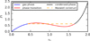 |
Fig. 1 van der Waals phase diagram for a fluid with Tr = 0.9. The gas phase and condensed phase are linked by the phase transition. As a negative |

2.2 Gravitational stability of fluids in a phase transition
The Jeans criterion (Jeans 1902) states that a fluid is gravitationally unstable if a perturbation has a wavelength larger than
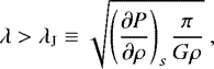 (7)
(7)
where  is the speed of sound cs squared, G the gravitational constant, P the pressure, ρ the density, and s the entropy.
In the case of a perfect gas,  , with γ the adiabatic index, kB the Boltzmann constant, T the temperature, and m the molecular weight. So for a perfect gas λJ is always positive; that is, there is always a scale below which the gas is gravitationally stable.
However,  with the adiabatic index γ > 0. Therefore, a fluid in a phase transition has
  (Maxwell’s construct), consequently λJ = 0. Formally, a fluid in a phase transition is gravitationally unstable even at microscopic scale.
2.3 Formation of condensations
The Jeans length (Eq. (7)) of an ideal gas is
 (8)
(8)
We showed (FP2015 and FP2016) that a fluid with λ > λJ,id collapses in a short time (Jeans time), heats up, and forms a gaseous body. This happens independently whether thefluid is in a pure gaseous phase or in a phase transition. On the other hand, if λ < λJ,id we need to distinguish between a pure gaseous fluid and a fluid in a phase transition. The former will remain gaseous, the perturbation being simply a sound wave.
Fluids in a phase transition, however, are always gravitationally unstable (see above). Small condensations quickly form due to the phasetransition. After a short period a new equilibrium is reached and the fluid has two phases, gaseous and solid. After that, the condensation fraction remains the same, but the grain size increases.
At first, the condensations only consist of a few molecules called oligomers. Thanks to dynamical friction, these oligomers attract each other and form bigger clumps, and the condensation size increases from snowballs, then comets, and up to planetoids. The final size of the solid body depends on the total mass, the solid mass fraction, and the formation timescale. The latter two are dependent on the density (see Sect. 4).
The accumulation of molecules towards oligomers and then larger bodies happens first by three-body interactions where one of the molecules carries away the excess energy. This leads to a temperature increase of the gaseous part of the fluid. However, this energy increase is only a fraction of the initial temperature (see Fig. A.1(B) and FP2015, FP2016), and gets smaller with increasing initial temperature. Therefore, the temperature does not exceed the critical value of H2. If there is rapid cooling, the fluid remains at its initial temperature.
A non-trivial result of our previous works is that the solid mass fraction Msolid∕Mtot is the same with or without gravity for phase transition fluids. The formation of larger bodies happens only by accumulating solid objects, and thus does not increase the solid fraction. In order to include phase transition effects in astrophysical hydrodynamical simulations it is therefore crucial to know this value for different densities and temperatures.
2.4 Paths to a phase transition state
The H2 phase transition happens well at typical temperatures (<33 K) for the cold ISM, but at very high densities (>1020 m−3) more typical of laboratory conditions. Thus, solid H2 is usually not expected to form directly in traditional collapse scenarios (one-step spherical collapse). However, two ingredients must be considered. Typical gravitational collapses occur along a sequence of geometries: first pancake (2D), then filament (1D), and finally point (0D) collapses (Lin et al. 1965; Zel’dovich 1970), and this in a recursive, fractal manner until the microphysics changes and reacts to the increased density and pressure. In FP2016, we discuss different collapsing geometries. A pancake or sheet-like collapse is not only the fastest collapsing geometry, but also leads at most to a doubling of temperature when density increases by more than a factor 100 in adiabatic conditions.
Cooling by radiation loss, depending on the opacity of the medium, leads to a smaller or negligible temperature increase. In addition, in sheet-like geometry the opacity increases only slightly, so reaching an optically thick condition is harder. Taking into account the multiscale, recursive nature of gravitational collapses, a cascade of collapses at higher and higher densities should proceed, allowing phase-transition conditions to be reached. Thus, a cascade of sheet-like, transparent to radiation collapses, combined with some cooling, can lead to a H2 phase transition. Along the cascade of collapses the specific angular momentum present in the initial density fluctuations must increase, increasingly favouring (as the scale decreases) the disk geometry instead of mere non-rotating pancake geometry.
Figure 2 shows the phase diagram of H2. A gas with typical properties of molecular clouds is compressed using different paths. While one-step filament- and point-like collapses lead to divergent temperatures, a sheet-like collapse without cooling only doubles the temperature. Assuming fast cooling, an increase of density without any temperature increase is conceivable, as the fluid opacity is not increased much during a sheet-like collapse. We also sketch the case of a cascade including partial cooling, which reaches a H2 phase transition after five recursive steps.
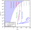 |
Fig. 2 Phase diagram of H2. Different adiabatic collapsing geometries and collapses including cooling are shown of a fluid with typical properties of a molecular cloud: T = 10 K, n = 1012 m−3. |
3 Simulations
Our goal is to calculate the solid mass fraction Msolid∕Mtot, the energy increase ΔEcond, and the timescale τcond of the formation of oligomers due to a phase transition. Figure 2 indicates the different temperature and densities of the simulations. The lower density limit is given by the needs of computing power: with decreasing density molecular encounters become rarer and the fraction Msolid∕Mtot lower. As a result, the time needed to reach a stable value for a fraction is much longer. In addition, to have a high enough resolution, more particles are needed. However, as we see in Sect. 4, we do reach sufficiently low densities in order to obtain a power law regime that allows us to extrapolate to lower densities with good confidence.
As described in more detail in FP2015 and FP2016, we use the popular molecular dynamics simulator LAMMPS (Plimpton 1995) to perform our simulations using the Lennard-Jones potential. As we want to calculate the fraction Msolid∕Mtot, which is independent of the strength of the gravitational potential, we do not need to include gravity in these simulations.
Most of the simulations have N = 105 molecules (see Sect. 4.1 for scaling), distributed initially randomly in a cube with periodic boundary conditions. We choose the volume V of the cube for different n = N∕V with number densities of log10(nr) = −6, −5.5, …, −1. The molecules have a Maxwellian velocity distribution with temperatures of log 10(Tr) = −1, −0.8, …, 0.4. The cut-off distance is rc = 4σ.
4 Results
Figure 3 shows a typical evolution of the solid mass fraction and kinetic energy increase during an adiabatic simulation. Both values follow an exponential law ∝ 1 − exp(−t∕τ), with time t and timescale τ. Once the simulation reaches a steady-state value, we measure the solid mass fraction and energy increase. These average values, ⟨Msolid⟩ and ⟨Δ Econd⟩, and the standard deviation are shown in Fig. A.1(A) and (B).
At high density and low temperature (especially log10(Tr) = −1 and − 0.8), there is a high fraction of condensations. These are the fluids which are “officially”, according to the van der Waals equation of state, in a phase transition. However, even fluids out of a phase transition, which have lower densities and/or higher temperatures, form a small amount of condensations.
The amount of condensations in phase transition fluids cannot be linked linearly to the density or temperature, as the intermolecular interactions are non-linear (∝ r−6 and r−12). The fluids out of a phase transition form condensations due to chance interaction between two or more molecules. The number of these interactions is linearly dependent on the density, and the probability of forming condensations increases with decreasing temperature. They follow a linear law:
 (9)
(9)
The simulations are adiabatic: the condensation formation implies a decrease in potential energy and therefore an increase in kinetic energy. One can recognize the similarities between the energy increase (Fig. A.1(B)) with the solid mass fraction (A): again the phase transition fluids are non-linear, but for fluids with low densities and/or high temperatures the energy of condensation follows a linear law
 (10)
(10)
where Ekin0 is the initial kinetic energy.
For all practical astrophysical uses, condensation should be considered an instantaneous process. Even simulations with many time steps (the simulations had up to 109 time steps) are orders of magnitude shorter than 1s in real time. We measure the condensation timescale by identifying the first appearance of ⟨Msolid⟩, and we average τ for all values up to that point. As seen in Fig. 3, the resulting value approximates the data rather well.
Figure A.1(C) shows the condensation timescales of the simulation for reaching the average ⟨Msolid⟩ value. No universal power law seems to govern the timescales. The timescales of low temperature fluids (Tr ≤ 10−0.4) follow an inverse power law:
 (11)
(11)
The timescales of high temperature fluids (T ≥ 10−0.2 Tc) follow an inverse square root law:
 (12)
(12)
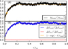 |
Fig. 3 Evolution of the solid mass fraction Msolid, kinetic energy increase ΔEcond, and total energy increase ΔEtot of the simulation with nr = 10−3.5, Tr = 10−0.6, and N = 105. ⟨Msolid ⟩ and ⟨Δ Econd⟩ are the average values and the error bars show the standard deviation. The extrapolation is ∝ 1 − exp(−t∕τ) with timescale τ. |
4.1 Scaling
In order to show the independence from the number of particles N, we ran several simulations with different values for N. Figure 4 shows the solid mass fraction, energy increase, and timescale as a function of N for such a simulation. All three values remain constant.
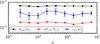 |
Fig. 4 Scaling of the simulation with nr = 10−3.5, Tr = 10−0.6, and differentnumbers of molecules N. Average values and standard deviation are shown for the solid fraction Msolid∕Mtot, condensation energy ΔEcond, and condensation timescale τcond. |
4.2 Extrapolation
The values of Msolid∕Mtot, Δ Econd, and τcond are non-linear for fluids in a phase transition. However, they can be extrapolated for fluids out of a phase transition. Fluids with temperatures of Tr = 0.1 are in a phase transition for densities down to ISM values (however, densities below 10−6nc cannot be simulated using molecular dynamics on today’s computers). Extrapolation laws are given for fluids with temperatures Tr > 0.1.
Least-squares extrapolations of the type alog10(n) + b for Msolid∕Mtot and ΔEcond show that a = 1 ± 0.05 ∀T. A linear approach is thus appropriate for these two laws. The least-square extrapolation for the condensation timescale τcond gives higher errors with a = −1 ± 0.2 for Tr ≤ 10−0.4, and a = −0.5 ± 0.2 for Tr ≥ 10−0.2.
We giveextrapolation laws for the timescales, but caution that they are speculative. This is not a large practical issue, however, as the linear laws overestimate the timescales, and even the extrapolated values for densities as low as the ISM are below one year.
The values for M(Tr), E(Tr), and Θ (Tr) are given in Table 1.
5 Conclusions
In astrophysical conditions, solid H2 formation can be seen as an instantaneous process with respect to gravitational processes. The solid mass fraction Msolid∕Mtot is high for fluids in a phase transition, ranging from 0.01 to >0.1. However, it does not drop to 0 for fluids out of a phase transition. A small fraction of the gas is always condensing as a result of the encounters of two or more molecules. The solid fraction is small and declines linearly with decreasing density. Nonetheless, even a mass fraction as small as 10−6 can make a difference, e.g. in planet formation where the ratio Mplanet∕M⊙ lies in the same range.
We present extrapolation laws to calculate the solid mass fraction Msolid∕Mtot and amount of energy increase ΔEcond due to the formation of oligomers for fluids out of a phase transition for temperatures from T =0.15 Tc to 2.5 Tc. The extrapolated values, together with the non-linear values for fluids in a phase transition from the simulations can be interpolated for subgrid physics in larger, continuous fluid simulations.
A phase transition in the ISM, especially the H2 transition inview of its high abundance, may have important dynamical implications which cannot be described using continuous physics, as is done in current simulation codes. Since in a phase transition all scales interact, and such a medium is always gravitationally unstable, the combination of gravity and phase transition is ideal to form bodies with sizes ranging from small oligomers to snowballs up to comet-sized bodies. Oligomers are seeds that facilitate the condensation of larger bodies on small scales, while gravitational condensations (clumps, spiral arms) on large scales combine with the phase transition scales to form bodies dominated by gravity (spherical bodies).
The ideal locations for condensing H2 in comet- or planet-sized bodies are cold starless cores, self-shielded from radiation in molecular clouds in the outskirts of galaxy disks where the local temperature should drop well below 10 K. Possibly bodies mostly made of H2 may form there and subsequently become a collisionless component of the disk until heating evaporates them, leaving heavier element bodies similar to comets.
Acknowledgements
This work is supported by the STARFORM Sinergia Project funded by the Swiss National Science Foundation. We thank the LAMMPS team1 for providing a powerful open source tool to the scientific community. We thank the referee for a thorough reading of the manuscript and constructive comments which substantially improved the paper.
Appendix A Additional figure
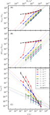 |
Fig. A.1 Simulation results for different temperatures Tr and number densities nr. The points show the average values, and the error bars show the standard deviation. (A) Solid mass fraction; (B) Temperature increase during condensation; and (C) Condensation time. |
References
- Air Liquide 1976, Gas Encyclopedia (Amsterdam: Elsevier) [Google Scholar]
- Belyanin, G. A., Kramers, J. D., Andreoli, M. A. G., et al. 2018, Geochim. Cosmochim. Acta, 223, 462 [NASA ADS] [CrossRef] [Google Scholar]
- Bolatto, A. D., Wolfire, M., & Leroy, A. K. 2013, Annu. Rev. Astron. Astrophys., 51, 207 [Google Scholar]
- Caillol, J. M. 1998, J Chem. Phys., 109, 4885 [NASA ADS] [CrossRef] [Google Scholar]
- Clerk-Maxwell, J. 1875, Nature, 11, 357 [NASA ADS] [CrossRef] [Google Scholar]
- Combes, F., & Pfenniger, D. 1997, A&A, 327, 453 [NASA ADS] [Google Scholar]
- Draine, B. T. 2011, Physics of the Interstellar and Intergalactic Medium (Princeton: Princeton University Press) [Google Scholar]
- Füglistaler, A., & Pfenniger, D. 2015, A&A, 578, A18 [NASA ADS] [CrossRef] [EDP Sciences] [Google Scholar]
- Füglistaler, A., & Pfenniger, D. 2016, A&A, 591, A100 [NASA ADS] [CrossRef] [EDP Sciences] [Google Scholar]
- Gahm, G. F., Grenman, T., Fredriksson, S., & Kristen, H. 2007, AJ, 133, 1795 [NASA ADS] [CrossRef] [Google Scholar]
- Gahm, G. F., Persson, C. M., Mäkelä, M. M., & Haikala, L. K. 2013, A&A, 555, A57 [NASA ADS] [CrossRef] [EDP Sciences] [Google Scholar]
- Gerhard, O., & Silk, J. 1996, ApJ, 472, 34 [Google Scholar]
- Grenier, I. A., Casandjian, J.-M., & Terrier, R. 2005, Science, 307, 1292 [NASA ADS] [CrossRef] [PubMed] [Google Scholar]
- Guilloteau, S., Piétu, V., Chapillon, E., et al. 2016, A&A, 586, L1 [NASA ADS] [CrossRef] [EDP Sciences] [Google Scholar]
- Hoyle, F., & Wickramasinghe, N. C. 1968, Nature, 218, 1124 [NASA ADS] [CrossRef] [Google Scholar]
- Jeans, J. H. 1902, R. Soc. London Philos. Trans. Ser. A, 199, 1 [Google Scholar]
- Johnston, D. C. 2014, Advances in Thermodynamics of the van der Waals Fluid (San Rafael, Morgan & Claypool Publishers) [Google Scholar]
- Kennicutt, R. C., & Evans, N. J. 2012, ARA&A, 50, 531 [NASA ADS] [CrossRef] [Google Scholar]
- Lin, C. C., Mestel, L., & Shu, F. H. 1965, ApJ, 142, 1431 [NASA ADS] [CrossRef] [Google Scholar]
- Lin, C. Y., Gilbert, A. T. B., & Walker, M. A. 2011, ApJ, 736, 91 [NASA ADS] [CrossRef] [Google Scholar]
- McKee, C. F., & Ostriker, E. C. 2007, ARA&A, 45, 565 [NASA ADS] [CrossRef] [Google Scholar]
- Meech, K. J., Weryk, R., Micheli, M., et al. 2017, Nature, 552, 378 [NASA ADS] [CrossRef] [Google Scholar]
- Pfenniger, D., & Combes, F. 1994, A&A, 285, 94 [NASA ADS] [Google Scholar]
- Pfenniger, D., Combes, F., & Martinet, L. 1994, A&A, 285, 79 [NASA ADS] [Google Scholar]
- Planck Collaboration XIX. 2011, A&A, 536, A19 [NASA ADS] [CrossRef] [EDP Sciences] [Google Scholar]
- Plimpton, S. 1995, J. Comput. Phys., 117, 1 [Google Scholar]
- Revaz, Y., Pfenniger, D., Combes, F., & Bournaud, F. 2009, A&A, 501, 171 [NASA ADS] [CrossRef] [EDP Sciences] [Google Scholar]
- Sandford, S. A., & Allamandola, L. J. 1993, ApJ, 409, L65 [NASA ADS] [CrossRef] [Google Scholar]
- van de Hulst, H. C. 1949, The Solid Particles in Interstellar Space (Utrecht: Drukkerij Schotanus & Jens) [Google Scholar]
- van der Waals, J. D. 1910, in Proc. Ser. B Phys. Sci. (Amsterdam: KNAW), 13, 1253 [Google Scholar]
- Walker, M. A. 2013, MNRAS, 434, 2814 [NASA ADS] [CrossRef] [Google Scholar]
- Wardle, M., & Walker, M. 1999, ApJ, 527, L109 [NASA ADS] [CrossRef] [PubMed] [Google Scholar]
- Wickramasinghe, N. C. 1968, Nature, 218, 661 [NASA ADS] [CrossRef] [Google Scholar]
- Zel’dovich, Y. B. 1970, A&A, 5, 84 [NASA ADS] [Google Scholar]
All Tables
All Figures
|
Fig. 1 van der Waals phase diagram for a fluid with Tr = 0.9. The gas phase and condensed phase are linked by the phase transition. As a negative |
| In the text | |
|
Fig. 2 Phase diagram of H2. Different adiabatic collapsing geometries and collapses including cooling are shown of a fluid with typical properties of a molecular cloud: T = 10 K, n = 1012 m−3. |
| In the text | |
|
Fig. 3 Evolution of the solid mass fraction Msolid, kinetic energy increase ΔEcond, and total energy increase ΔEtot of the simulation with nr = 10−3.5, Tr = 10−0.6, and N = 105. ⟨Msolid ⟩ and ⟨Δ Econd⟩ are the average values and the error bars show the standard deviation. The extrapolation is ∝ 1 − exp(−t∕τ) with timescale τ. |
| In the text | |
|
Fig. 4 Scaling of the simulation with nr = 10−3.5, Tr = 10−0.6, and differentnumbers of molecules N. Average values and standard deviation are shown for the solid fraction Msolid∕Mtot, condensation energy ΔEcond, and condensation timescale τcond. |
| In the text | |
|
Fig. A.1 Simulation results for different temperatures Tr and number densities nr. The points show the average values, and the error bars show the standard deviation. (A) Solid mass fraction; (B) Temperature increase during condensation; and (C) Condensation time. |
| In the text | |
Current usage metrics show cumulative count of Article Views (full-text article views including HTML views, PDF and ePub downloads, according to the available data) and Abstracts Views on Vision4Press platform.
Data correspond to usage on the plateform after 2015. The current usage metrics is available 48-96 hours after online publication and is updated daily on week days.
Initial download of the metrics may take a while.