| Issue |
A&A
Volume 612, April 2018
|
|
|---|---|---|
| Article Number | A45 | |
| Number of page(s) | 15 | |
| Section | Stellar atmospheres | |
| DOI | https://doi.org/10.1051/0004-6361/201731633 | |
| Published online | 20 April 2018 | |
PEPSI deep spectra
II. Gaia benchmark stars and other M-K standards★
Leibniz-Institute for Astrophysics Potsdam (AIP),
An der Sternwarte 16,
14482
Potsdam, Germany ; ;
e-mail: This email address is being protected from spambots. You need JavaScript enabled to view it.
; This email address is being protected from spambots. You need JavaScript enabled to view it.
; This email address is being protected from spambots. You need JavaScript enabled to view it.
Received:
24
July
2017
Accepted:
22
November
2017
Abstract
Context. High-resolution échelle spectra confine many essential stellar parameters once the data reach a quality appropriate to constrain the various physical processes that form these spectra.
Aim. We provide a homogeneous library of high-resolution, high-S/N spectra for 48 bright AFGKM stars, some of them approaching the quality of solar-flux spectra. Our sample includes the northern Gaia benchmark stars, some solar analogs, and some other bright Morgan-Keenan (M-K) spectral standards.
Methods. Well-exposed deep spectra were created by average-combining individual exposures. The data-reduction process relies on adaptive selection of parameters by using statistical inference and robust estimators. We employed spectrum synthesis techniques and statistics tools in order to characterize the spectra and give a first quick look at some of the science cases possible.
Results. With an average spectral resolution of R ≈ 220 000 (1.36 km s−1), a continuous wavelength coverage from 383 nm to 912 nm, and S/N of between 70:1 for the faintest star in the extreme blue and 6000:1 for the brightest star in the red, these spectra are now made public for further data mining and analysis. Preliminary results include new stellar parameters for 70 Vir and α Tau, the detection of the rare-earth element dysprosium and the heavy elements uranium, thorium and neodymium in several RGB stars, and the use of the 12C to 13C isotope ratio for age-related determinations. We also found Arcturus to exhibit few-percent Ca II H&K and Hα residual profile changes with respect to the KPNO atlas taken in 1999.
Key words: stars: atmospheres / stars: late-type / stars: abundances / stars: activity / stars: fundamental parameters
Based on data acquired with PEPSI using the Large Binocular Telescope (LBT) and the Vatican Advanced Technology Telescope (VATT). The LBT is an international collaboration among institutions in the United States, Italy, and Germany. LBT Corporation partners are the University of Arizona on behalf of the Arizona university system; Istituto Nazionale di Astrofisica, Italy; LBT Beteiligungsgesellschaft, Germany, representing the Max-Planck Society, the Leibniz-Institute for Astrophysics Potsdam (AIP), and Heidelberg University; the Ohio State University; and the Research Corporation, on behalf of the University of Notre Dame, University of Minnesota and University of Virginia.
© ESO 2018
1 Introduction
High-resolution spectroscopy is key for progress in many fields of astrophysics, most obviously for fundamental stellar physics. The advent of ESA’s Gaia mission spurred a large high-spectral-resolution survey of FGK-type stars at ESO with significant results now coming online (e.g., Smiljanic et al. 2014). This survey, dubbed the Gaia-ESO survey (Gilmore et al. 2012), also defined a list of 34 benchmark FGK stars in both hemispheres (Blanco-Cuaresma et al. 2014) that were analyzed with many different spectrum-synthesis codes and with data from different spectrographs. The analysis focused, among other topics, on global stellar parameters like effective temperatures and gravities (Heiter et al. 2015), metallicity (Jofré et al. 2014) and chemical abundances (Jofré et al. 2015), and on some stars in detail (e.g., Creevey et al. 2015 on HD 140283). A recent addition to low-metallicity stars was presented by Hawkins et al. (2016).
One of the major conclusions from this program is that even for main sequence stars the spectroscopically determined quantities may differ significantly with respect to the fundamental value obtained from direct radius and flux measurements. But even within the spectroscopic analyzes the global parameters Teff, logg, and metallicity, along with micro- and macroturbulence and rotational line broadening, differ uncomfortably large (see, for example the discussion in Heiter et al. 2015). Among the least cooperative stars appear to be the giants and metal-poor dwarfs. Comparisons indicate, for example that for solar-metallicity giants with Teff ≈ 5000 K and logg ≈ 2.8, the spectroscopic approach can lead to overestimated gravities. Intrinsic line-profile variability may become the limit for precision, in particular due to (non-detected) p-mode oscillations for the K giants and rotationally-modulated stellar activity (spots, faculae, etc.) for all of the cool stars. Besides intrinsic stellar variability, one extra source of uncertainty is the remaining blending situation with weak molecular lines due to finite spectral resolution.
The data in the Gaia benchmark spectral library provided by Blanco-Cuaresma et al. (2014) were originally homogenized to the highest minimum spectral resolution of the different spectrographs involved, and corresponded in practice to R = λ∕Δλ = 70 000. The vast majority of the spectra for the benchmarks are from HARPS (Mayor et al. 2003) with an original resolution of 115 000. NARVAL spectra (Auriére 2003) have an average resolution of 65 000 (Paletou et al. 2015), and the UVES data (Dekker et al. 2000) have 78 000–115 000. Peak signal-to-noise ratios (S/N) of between 150 to 824 were achieved. Higher S/N was obtained for eight bright stars in the UVES-POP library (Bagnulo et al. 2003) but with the lower spectral resolution of ≈80 000. Yet, if some of the most decisive astrophysical processes for stellar variability, that is, stellar convection, is to be detected and characterized in spectra, it requires much higher spectral resolution and even higher S/N, and thus even larger telescopes. Most of the stars analyzed in work previous to the Gaia-ESO survey had even lower resolution than the minimum resolution for the benchmark stars, for example the bright M-giantγ Sge with 50–60 000, which is still the typical spectral resolution for a fixed-format échelle spectrograph on a smaller telescope.
We havejust put into operation the optical high-resolution échelle spectrograph PEPSI (Potsdam Echelle Polarimetric and Spectroscopic Instrument) at the currently largest aperture optical telescope in the world; the effective 11.8 m Large Binocular Telescope (LBT; Hill et al. 2012). PEPSI provides a spectral resolution of up to 270 000 for the wavelength range 383–912 nm and can alternatively be fed by the nearby 1.8 m Vatican Advanced Technology Telescope (VATT) or by a small solar disk integration (SDI) telescope. The instrument is described in detail in Strassmeier et al. (2015) and we refer to this paper for technical and operational details. Solar flux spectra with PEPSI were presented and analyzed in paper I (Strassmeier et al. 2018), where we also described the data reduction in more detail. A further application is presented in paper III to Kepler-444 (Mack et al. 2018).
The current paper presents first PEPSI spectra for 48 bright stars including those of the original 34 Gaia benchmark stars that were observable from the northern LBT site. Data were taken during several instrument commissioning runs throughout 2015 until March 2017. Peak S/N of several thousand in the red wavelength regions were achieved with average-combining individual exposures. All these spectra are extremely rich in detail and therefore are made public for further data mining and analysis. Science-ready FITS files of the average-combined spectra are available for download1 and raw data may be requested. Section 2 describes the observations and the spectrograph while Sect. 3 briefly reiterates the data reduction. Section 4 gives a first quality assessment of the data product. The stellar sample and its science cases with a few additions to the original Gaia benchmark stars are discussed in Sects. 5 and 6, respectively. Section 7 is a summary.
2 Observations
High-resolution spectra with R = λ∕Δλ between 200 000 and up to 270 000 were obtained with PEPSI (Strassmeier et al. 2015) at the 2 × 8.4 m LBT (Hill et al. 2012). PEPSI is a fiber-fed white-pupil échelle spectrograph with two arms (blue and red optimized) covering the wavelength range 383–912 nm with six different cross dispersers (CD). The instrument is stabilized in a pressure and thermally controlled chamber and is fed by three pairs of octagonal fibers per LBT unit telescope (named SX and DX). The different core diameters of the fibers and their respective image slicers set the three different resolutions of the spectrograph (43 000, 120 000 and 250 000). In use for this paper was image slicer block #2. Its 250 000-mode, which was used for the spectra in this paper, is made possible with the seven-slice image slicers and a 100-μm fiber with a projected sky aperture of 0.74′′, comparable to the median seeing of the LBT site. Its resolution element is sampled with two pixels. One resolution element corresponds to 1.2 km s−1 for the resolving power of 250 000. Two 10.3 k × 10.3 k STA1600LN CCDs with 9-μm pixels record a total of 92 échelle orders in six wavelength settings. The dispersion changes from 8 mÅ/pixel at 400 nm to 18 mÅ/pixel at 900 nm and results in a ≈430 000 pixel long spectrum with unequally spaced step size. An example spectrum is shown in Fig. 1.
The six wavelength settings are defined by the six cross dispersers (CD I to VI), three per arm and two always simultaneously. It takes three exposures to cover the entire wavelength range 383–912 nm. Several of the spectra extend out to 914 nm because we repositioned cross disperser VI during commissioning and then gained another échelle order. Any of the three resolution modes can be used either with sky fibers for simultaneous sky and target exposures or with light from a stabilized Fabry–Pérot etalon (FPE) for simultaneous fringe and target exposures for precise radial velocities (RV). However, the short integrations for the targets in this paper made the use of the sky fibers obsolete. Therefore, all spectra in this paper were taken in target+target mode, i.e., without simultaneous sky or FPE exposures, leaving two simultaneous target spectra on the CCD (one from each of the 8.4 m LBT unit telescopes). We always refer to the combined target+target spectrum when referring to “an LBT spectrum”, e.g. for example in the number of spectra in the tables. The SDI telescope makes use of PEPSI during day time and also consists of two spectra per exposure. Paper I in this series dealt with these spectra. A 450-m fiber feed (Sablowski et al. 2016) from the 1.8 m VATT was used for very bright stars on several occasions. We note that the VATT spectra consist of just a single target spectrum on the CCD because it is only a single telescope.
Table A.1 summarizes the detailed observing log and identifies the individual spectra. Observations with the LBT were conducted during the epochs April 1–2 and 8–10, May 23–25, September 25 and 27, and November 19, in 2015; during June 2-4 and September 29–30 in 2016; and on March 3, 2017. Observations with the VATT were done during the epochs April 1–7, May 1–10, May 26–June 1, June 17–24, in 2015, and April 2–9 and May 24–June 2 in 2016. At around mid November 2015 the Blue CCD developed a bad amplifier (amp #5) affecting a section of 5000 × 1280 pixels on the CCD. It resulted in a drastically degraded quantum efficiency and practically in a loss of the three halves of the respective échelle orders that fell on this CCD section. This was repaired in early 2016 and the affected wavelength region was re-observed for some of the stars (but at a grossly different epoch). The spectrograph was in different states of alignment and focus and thus resulted in slightly different dependencies of spectral resolution vs wavelength. Also, acceptable barometric stability of the chamber was not achieved until summer 2015.
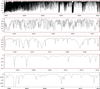 |
Fig. 1 Example spectrum of 70 Vir, spectral type G4 V–IV (x-axis is wavelength in Angstrom, y-axis is relative intensity). Top: full 5290-Å wavelength coverage. The other panels show magnifications of four selected wavelength regions. Top down: numerous Fe I lines around 4250 Å, the Mg I triplet at 5175 Å, the Li I 6708-Å region, and the 8004-Å line region commonly used for 12 C / 13C determination. |
3 Data reduction
PEPSI data reduction was described in detail in paper I. The Sun is the only target where we can compare to even higher quality data from Fourier Transform Spectrographs (e.g., Wallace et al. 2011; Reiners et al. 2016). The stellar PEPSI data in the present paper do not differ principally from the solar PEPSI data except for the S/N. This allows a direct comparison of solar flux spectra with stellar spectra because the solar light passes through exactly the same optical path as the stellar light. A full-wavelength PEPSI exposure in the R = 250 000 mode is always merged from seven (image) slices per échelle order, 17 échelle orders per cross disperser, and two arms recorded with two different CCDs optimized for blue and red response.
The data were reduced with the Spectroscopic Data System for PEPSI (SDS4PEPSI) which is a generic software package written in C++ under a Linux environment and loosely based upon the 4A software (Ilyin 2000) developed for the SOFIN spectrograph at the Nordic Optical Telescope. It relies on adaptive selection of parameters by using statistical inference and robust estimators. The standard reduction steps include bias overscan detection and subtraction, scattered light surface extraction from the inter-order space and subtraction, definition of échelle orders, optimal extraction of spectral orders, wavelength calibration, and a self-consistent continuum fit to the full 2D image of extracted orders. Every target exposure is made with a simultaneous recording of the light from a Fabry–Pérot etalon through the sky fibers. For the spectra in this paper, the Fabry–Pérot wavelength solution was not implemented. Instead, exposures with a standard Thorium–Argon (Th-Ar) hollow-cathode lamp were used for the wavelength calibration. Its solution is based on about 5000 spectral lines from all seven image slices and all spectral orders. A 3D Chebychev polynomial fit achieves an accuracy of about 3–5 m s−1 in the image center with a rms of about 50 m s−1 across the entire CCD. The Th-Ar calibration images are taken during daytime before the observing night and the wavelength scale zero point of the science images is thus relying on the stability of the PEPSI chamber. Wavelengths in this paper are given for air and radial velocities are reduced to the barycentric motion of the solar system. We note that the spectra in the present paper were reduced and extracted just like the Sun-as-a-star data in paper I with the only difference that the continuum normalization was adjusted to the spectral classification.
In order to achieve the high S/N, we employ a “super master” flat-fielding procedure that is based on a combined flat-field image made from ≈2000 individual images taken during daytime. Individual stellar spectra are first flat fielded, then extracted, and then average combined with a χ2 minimization procedure weighted with the inverse variance in each CCD pixel. For three taps on the STA1600LN CCDs surface, the pixel response is a function of the exposure level. This blemish is dubbed fixed-pattern noise and described in detail in paper I. In order to achieve very high S/N, all raw images are corrected for nonlinearity of each CCD pixel vs its ADU level with the use of the super master flat field image. It comprises a polynomial fit of the CCD fixed-pattern response function in 70 de-focused flat field images at different exposure levels. Each of such an image is again the sum of 70 individual exposures made in order to minimize the photon noise. The fixed-pattern response function is the ratio of the flat field image and its 2D smoothed spline fit which removes all signatures of the de-focused spectral orders. The accuracy of this correction allows reaching a S/N in the combined spectra of as high as 4500. Because the pattern shows a spatial periodicity with a spacing of 38 pixels, which is wavelength dependent on the red CCD (but not on the blue CCD), it leaves residual ripples with a periodicity of 38 pixels in the spectrum. It is being removed to the best possible level but the residual pixel-to-pixel non uniformity after the super master flat division currently limits the effective S/N from the affected CCD taps to ≈1300:1. Other regions are unaffected.
4 Data product
4.1 Building deep spectra
Deep spectra in this paper are build by average-combining individual spectra, usually taken back-to-back within a single night. For some targets individual spectra are from different nights or even different runs. The observing log is given in Table A.1. Any spectrum co-addition is prone to variations of the entire spectrograph system, including errors from the seeing-dependent fiber injection or the temperature-sensitive CCD response or the optical-path differences due to the LBT being two telescopes and/or when using the VATT as the light feed.
When two spectra from different LBT sides are combined, the spectra are re-sampled into the wavelength grid of the first spectrum, then they are averaged with their corresponding weights (inverse variance in each pixel). First, the optimally extracted spectra from every slice of the image slicer are combined into a single spectrum for each spectral order. Prior to its averaging, all spectra are re-sampled into the common wavelength grid of the middle slice. The wavelength in each pixel is defined by the Th-Ar wavelength solution and remains unequally sampled. Then, the two average spectra from the two sides of the LBT telescope are combined into a single spectrum with the weighted average to the common wavelength grid of the first spectrum. One spectrum is re-sampled to the other by means of spline interpolation.
Because the spectra are normalized to a pseudo-continuum I∕Ic , there is no need to re-scale them in intensity and the final continuum level will be adherent to the one with the higher S/N. The very same procedure is applied for building the average-combined deep spectra. For more details we refer to paper I.
4.2 Intrinsic spectrum variations
A deep spectrum may be affected by intrinsic stellar changes, for example due to rotational modulation by spots and plages, non-radial surface oscillations, or Doppler wobbling due to unseen stellar companions or exoplanets. However, exposure times are usually rather short compared to the typical stellar variability timescales. When using the LBT the exposure times are typically just tens of seconds up to a few minutes but exposure times with the VATT and its 450-m fiber link can be up to 60 min. Nevertheless, even after adding the CCD read-out overhead of 90 s and the co-adding of, say, typically four spectra, the total time on target still sums up to a relatively short period in time, typically just tens of minutes for the LBT data and up to a maximum of 3 h for the VATT targets. Any intrinsic changes with a timescale significantly longer than this we can safely dub non critical. This is certainly the case for rotational modulation and the revolution of orbital companions where we expect periods in excess of many days up to thousands of days. An example is α Tau, which shows RV variations of up to 140 m s−1 with a period of 629 d due to a super-Jupiter companion as well as rotational modulation with a period of 520 d (Hatzes et al. 2015).
Solar-like non-radial oscillations act on much shorter time scales than rotation and were discovered in several of our targets, for example for η Boo (Kjeldsen et al. 2003). Frandsen et al. (2002) detected oscillation periods of as short as 2–5 h in the giant ξ Hya, another target in this paper. Just recently, Grundahl et al. (2017) identified 49 pulsation modes in the G5 subgiant μ Her, originally discovered by Bonanno et al. (2008) as an excess of power at 1.2 mHz. There is also evidence that sub-m s−1 RV oscillations of as short as 50 min were found in HARPS spectra of the active subgiant HR 1362 (Dall et al. 2010) (not part of the target list in this paper). While the solar 5-min oscillation produces only a disk-averaged full RV amplitude of order 0.5 m s−1 (see paper I, but also Christensen-Dalsgaard & Frandsen 1983; Probst et al. 2015), this amplitude could amount to tens of m s−1 for K and M giants. For example, Kim et al. (2006) found α Ari to be a pulsating star with a period of 0.84 d and a RV amplitude of 20 m s−1 while Hatzes et al. (2012) found for β Gem up to 17 pulsation periods with individual RV amplitudes of up to 10 m s−1 . A mix of rotational and orbital, and pulsation periods of 230 d and 471 d, respectively, were found for the single-lined M0 giant μ UMa (Lee et al. 2016).
In case there are line-profile and RV changes in our targets due to radial or non-radial oscillations, we would then obtain an intrinsically averaged spectrum. For one of the late-type giant targets, β UMi (K4III), Fig. 2 shows a visual comparison of all 22 individual spectra (from 11 consecutive back-to-back exposures in binocular mode) with its combined spectrum. Only a single spectral line is shown; K I 7699 Å (loggf = −0.176, χ = 1.6 eV). Panels a and b are for two levels of magnified details, while the right panel c shows the S/N per pixel just for the line core. Note that the zoom factor in the plot in Fig. 2b is considerable; all there is shown is a 0.08-Å region centered at the K I-7699 line core. The width of the entire plot is approximately one spectral resolution element of UVES or HARPS. We chose this line because of its absorption components from the local interstellar medium (LISM) which, if present, may be used as a reference with respect to the stellar photospheric contribution. No such LISM lines are seen in β UMi. Not unexpected, the largest spread of intensity is found with a 0.3% peak-to-valley (p-v) after 15 min on target (rms of 0.1%), sampled with 11 consecutive 15-s exposures with both LBT telescopes. For the line core, this spread is expected for the data quality of a single exposure of typical S/N of ≈200 in the K I-line core. The average-combined spectrum has a S/N of 2250 in the continuum on both sides of the line and still around 900 in the line core itself (Fig. 2c). Therefore, a p-v spread of 0.3% near the continuum is a significant deviation with respect to the photon noise and is likely due to the combined effects of remaining systematic errors (mostly continuum setting) and yet unverified intrinsic stellar variations, presumably non-radial pulsations.
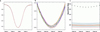 |
Fig. 2 Comparison of an average-combined spectrum and its individual exposures for β UMi (K4III). Thex-axes are wavelengths in Å. The 22 individual exposures are shown as lines, the average combined “deep spectrum” as dots. Panel a: a 0.8-Å section showing the 22 exposures of the K I 7699 Å line profile. The y-axis is relative intensity. No differences can be seen at this plot scale. Panel b: a zoom into a 0.08-Å subsection of the line core. The spacing of the dots represent the CCD pixel dispersion. Panel c: S/N per pixel in the K I line core for the same spectral window as in panel b. |
4.3 Signal-to-noise ratio
Table 1 lists the S/N for the deep spectra. S/N is always given for the continuum and per pixel at the mid wavelength of each cross disperser. The variance of each CCD pixel in the raw image is originally calculated after bias subtraction given the measured CCD gain factor for each of the 16 amplifiers of the STA1600LN CCD. The original variance is then propagated at every data reduction step and its final value is used to determine the S/N in every wavelength pixel of the final continuum normalized spectrum. The number of individual spectra employed for a deep-spectrum varies from star to star and is given in the last column of Table 1. It may differ from Table A.1 because not always all existing spectra wereincluded for the combined average spectrum. In case of bad seeing when spectra had significantly lower S/N, or when we had better spectra from different epochs, we simply did not use all of the available spectra but still list them in Table A.1. Several of our dwarf stars (HD 84937, HD 189333, HD 101364, HD 82943, HD 128311, and HD 82106) have S/N below 70:1 at the mid wavelength of CD-I at 400 nm and are thus not recommended for a quantitative analysis at these wavelengths. Note that due to the relatively small fiber entrance aperture of 0.74′′ the S/N strongly depends on seeing. Blue-arm spectra that were taken only with the VATT and its 450 m fiber generally have lesser S/N. The fibre transmission at 500 nm is 30% (see Strassmeier et al. 2015, their Fig. 41).
Figure 3a is a plot of a typical distribution of S/N across wavelength for one of the targets. Note that wavelength regions at the edges of spectral orders repeat in adjacent orders. Because the order merging procedure in our SDS4PEPSIpipeline is a weighted average of the overlapping wavelength regions, the S/N for these strips of wavelength is a weighted average from two different orders and thus formally higher than the rest, but not necessarily more accurate due to continuum-setting uncertainties.
Stellar sample of deep PEPSI spectra.
4.4 Spectral resolution
As in any échelle spectrograph, the resolution changes along and across each spectral order due to the change of the optical image quality and the anamorphism of the grating. The optical design of PEPSI includes a small 0.7° off-plane angle of the incident beam, which results in a small tilt of 4° of the spectral lines formed by the image slicers. This tilt is compensated by a fixed counter-rotation of the entire imageslicer. The residual tilt of the slices that are further away from the optical axis is of the order of 1°, which degrades the resolving power only by ≈2%. The main contributor to the resolving power variations in PEPSI is the change of the optimal focus position across the large area of the two 10 k CCDs.
The nominal spectrograph resolving power vs wavelength was shown in our paper I. The true resolution varied from run to run, in particular for the data taken during commissioning because the line FWHM and, thus, the resolution is computed from the Th-Ar lines at the focus positions achieved at that time. Specifically, we calculated the resolving power for every Th-Ar emission line from its FWHM in pixels and the dispersion at the line position derived from the 3D dispersion polynomial. The best focus position is selected as the maximal median resolving power of all spectral orders vs focus position. An example for July 2016 is shown in Fig. 3b. Focus sequences for every observing run and for all CDs were made with the Th-Ar cathode as the light source. A FFT auto-correlation for a central region on the CCD with 3000 × 300 pixels is applied for focus determination, its FWHM is then converted to effective spectral resolution as a function of wavelength. Our spectra in this paper were all taken with a focus selected to suit all CDs at once. One could do a wavelength dependent focus, that is, refocus for every CD combination, but that was not done for the present data. Therefore, the average resolution for the stars in this paper falls mostly short of λ∕Δλ of 250 000 with a range from 180 000 near the blue cut-off to a peak of 270 000 near 700 nm. The grand average from 383 to 912 nm is approximately 220 000 or 1.36 km s−1 . When modeling individual spectral regions, or line profiles, it is advisable to consult Fig. 3b or the FITSheader for the true resolution at a particular wavelength. Resolution dispersion is approximately ±30 000 for the entire 383 to 912 nm range.
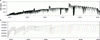 |
Fig. 3 Examples for the typical S/N and spectral resolution of the library stars in this paper. Panel a: S/N of the deep spectrum of the G4 subgiant 70 Vir. The larger S/N in the very red wavelengths is mostly due to the larger number of individual spectra. Note that the local peaks in S/N are due to the wavelength overlap of the cross dispersers, which effectively doubles the number of pixels there. Panel b: spectral resolution for the focus achieved for the July 2016 run. |
4.5 Continuum
Continuum-setting errors are among the largest uncertainties for high-resolution spectroscopy. It is particularly problematic for cool stars where line blanketing effectively removes any clean continuum signature. This is typical for blue wavelengths short of ≈450 nm as well as those red wavelengths that are affected by the wide terrestrial O2 absorption bands. It is generally the case for M stars due to increasing molecular bands with decreasing effective temperature. For solar-like stars in this paper, we referenced to the dry NSO FTS solar spectrum for continuum definition just like we did in paper I for the Sun itself. For ≈K1 giants, we use as a reference the KPNO Arcturus atlas from Hinkle et al. (2000). The final continuum is obtained from synthetic spectra. We tabulated synthetic spectra generated with the MARCS model atmospheres (Gustafsson 2007), the VALD atomic line list (Kupka et al. 2011), the SPECTRUM code (Gray & Corbally 1994), and the atmospheric parameters from the literature (taken from Blanco-Cuaresma et al. 2014). These synthetic spectra are first trimmed to the reference stars (Sun and Arcturus) and then employed to build a continuum free of spectral lines, which is then used for division for all targets of the atlas. We noticed a systematic opacity deficiency for giant-star spectra near our blue cut-off wavelength. Currently, we bypassed this by fitting the Arcturus atlas and deriving a fudge parameter that is then multiplied with the synthetic continuum.
There will always be residual continuum errors left in the data. For the red spectra these are generally caused by the increasing telluric contamination toward longer wavelengths. Although a small effect, it can cause systematic shifts at some wavelength regions of the order of 1%. However, such small shifts may simply be compensated posteriori to the data reduction. More problematic is the line blanketing in the blue together with the lowered S/N of the blue spectra in general. It can lead to continuum errors of 10–20% for the regions bluer than 397 nm. Targets with very low S/N near the blue cutoff wavelength may appear with line depths that are negative and peaks that are above continuum. When comparing these PEPSI spectra to synthetic spectra it is advisable to also refit the continuum level in question.
4.6 RV zero point
In paper I, we have shown that our absolute RV zero point was within a rms of just 10 m s−1 of the HARPS laser-comb calibrated solar atlas (Molaro et al. 2013). This allows us to combine spectra taken over a long period of time, at least as long as the spectrograph chamber is not opened. Besides, there is a small systematic difference of on average 9 m s−1 between the zero points of LBT SX and LBT DX spectra due to its separate light coupling. The shift between SXand DX is not a single constant but depends on the CD, ranging between 5 to 30 m s−1. The major contribution is because SX and DX have different foci, hence the stellar images can be offset from one another. We will investigate further whether the shift can be compensated with the simultaneous FPE reference source. For the present paper, any differential RV shifts were removed for each individual CD by means of a least-squares minimization with respect to the SX side. Larger than expected shifts occurred during commissioning because we realigned the CDs once in the blue arm and twice in the red arm, and the spectrum image had unavoidably moved on the detector. Despite that these data periods were treated with special attention, it created residual RV inhomogeneities of the order of the uncertainties themselves. Because we do not intend to provide RVs for the library stars, we shifted all spectra in this library to their respective barycentric RV value by subtracting the RV given in the header of the respective FITS file. This shall enable easier inter comparisons. The date given in the average combined FITS file is the average date resulting from the combination of the individual CDs, it has no physical meaning.
4.7 Wavelength coverage
The free spectral range for each CD has been graphically shown in our technical paper in Strassmeier et al. (2015) as well as in paper I, and we refer the reader to these papers for more details. Here we recap the wavelength coverage in nm for each cross disperser; CD-I 383.7–426.5, CD-II 426.5–480.0, CD-III 480.0–544.1, CD-IV 544.1–627.8, CD-V 627.8–741.9, and CD-VI 741.9–912. All spectra in this paper cover the full wavelength range 383–912 nm. Because of the comparably low efficiency in the bluest cross disperser (CD-I), and the accordingly longer exposure times, its exposures had sometimes to be done on different nights for some targets. For a total of six dwarf-star targets, we lacked the telescope time to redo the CD-I exposure with an appropriate longer integration time (see Sect. 4.3). Their initial spectra provided only poor S/N for wavelengths shorter than or around Ca II H&K, and we recommend not to use these wavelength sections for the six stars. For one of these target, HD 82106, we did not include the spectrum shorter than 398 nm because it affected the continuum setting for the remaining wavelengths of CD-I. For the other five stars, we decided to keep these wavelengths in the library for the sake of completeness. Note that the bluest wavelength regions are not accessible with the VATT because of the 450-m fibre link and its effectively 95% absorption loss at 400 nm. The stars affected can also be identified in Table A.1 by their two-digit S/N for CD I/404 nm.
4.8 Blemishes
Four stars observed in the time frame November–December 2015 have only a fractal wavelength coverage in the blue arm. On Nov. 13, 2015, we discovered a degrading amplifier in the blue 10k CCD that left its section on the CCD (approximately 5000 × 1280 pixels) with an effective gain of 1.2 instead of 0.5. This in turn resulted in a non-linear behavior at our exposure levels and lowered the quantum efficiency, which both caused intensity jumps in the spectrum at the amplifier edges and thus confused the order tracing algorithm of the data reduction. It affects one half of altogether three échelle orders. The jumps were corrected and spectra extracted but with approximately half the S/N for the regions affected. The chip was repaired in early 2016 and the problem did not occur again (bonding at the CCD had gotten loose and introduced a variable ohmic resistance). The consequence of this is that we do not recommend to use the wavelength regions of this section of the blue CCD of the four stars (51 Peg, 7 Psc, α Ari, and α Cet), which were all taken during above time window. Table 2 lists the detailed wavelengths affected.
Several of the spectra show a (time-variable) HeNe-laser emission line at 6329 Å. This line was picked-up accidentally as stray light from the LBT laser tracker system (which should have been turned off). Its FWHM is around 53 mÅ and its shape appears rather asymmetric with an emission intensity of up to 1.4 relative to the (stellar) continuum. Spectra are usually not affected unless the laser line falls within a stellar line like, for example in the 61 Cyg A spectra taken during the May 2015 run.
Wavelength regions in Å that are affected by a bad-amplifier problem with the Blue CCD for the epoch November–December 2015.
4.9 A comparison with the KPNO Arcturus atlas
Hinkle et al. (2000) assembled an atlas spectrum of Arcturus from a large number of individual spectral segments obtained with the KPNO coudé feed telescope and spectrograph at Kitt Peak. It took 15 nights to complete all exposures (from Apr. 20 to June 13, 1999). Its spectral resolution ranges between 130 000 to 200 000 for the wavelength range 373 to 930 nm and has been an outstanding reference for more than a decade. It succeeded the photographic Arcturus atlas of Griffin (1968).
We employ the KPNO atlas spectrum to find its continuum and use it for PEPSI division. Then, the PEPSI spectrum matches the KPNO spectrum almost perfectly. Figure 4a shows a comparison of the KPNO atlas and the PEPSI spectrum for the Fraunhofer G-band. PEPSI’s slightly higher spectral resolution shows up with slightly deeper lines, on average 0.5% deeper than the KPNO lines (in particular in the red wavelengths). The wavelength distribution of the achieved S/N is rather inhomogeneous for the PEPSI spectrum because CD-III was employed for only four short VATT exposures while CD-VI had included nine LBT exposures (exposure time with the LBT was 3 s, with the VATT 4 min for similar S/N). Red ward of ≈400 nm the photon noise is not noticeable anymore in the plots, peaking at 6000:1 at 710 nm, but is inferior than the KPNO atlas for the very blue parts shorter than ≈397 nm, where values below 100:1 are reached.
The wavelength zero point of the KPNO and the PEPSI spectra differs by several hundred m s−1 . A cross correlation of each PEPSI spectrum with the appropriate part of the KPNO atlas suggests the following shifts PEPSI-minus-KPNO in m s−1 (CD-I 545, CD-II 631, CD-III 576, CD-IV 740, CD-V 783, and CD-VI 871). Note that the higher differences for the red CDs are due to the increase of telluric lines in these wavelength regions which makes the cross correlation more prone to systematic errors. When comparing the two spectra these shifts were applied so that both spectra are in barycentric rest frame. The pixel-to-pixel ratio spectrum (PEPSI spectrum divided by the KPNO atlas) is in general dominated by the variable water content of Earth’s atmosphere which creates numerous artifacts. Three wavelength sections containing the Ca II H line core, Hα, and Li I 6708 are shown in Fig. 4b. The presence of emission in the cores of these lines is a simple diagnostic of magnetic activity in the chromospheres of late-type stars. As can be seen in Fig. 4b, the ratio spectrum shows weak differences in the Ca II H and Hα profiles at a few per cent level (10% peak-to-valley in the H&K line core and 8% in Hα). Note that the time difference between the KPNO spectrum and the PEPSI spectrum is 16 years. We usually interpret such residual emission due to changing magnetic activity. While just a preliminary result, it supports the earlier claims of the existence of both Ca II H&K variability (with a period of ≤14 yr) by Brown et al. (2008) and the detection of a (very weak) longitudinal magnetic field by Hubrig et al. (1994) and Sennhauser & Berdyugina (2011).
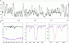 |
Fig. 4 Comparison of the deep PEPSI spectrum of Arcturus with the KPNO Arcturus atlas from Hinkle et al. (2000). Panel a: numerous CH lines centered around the Fe I/Ca I blend at 4308 Å that constitute the Fraunhofer G-band. The dots are the PEPSI spectrum and the line is the KPNO atlas. The match is nearly perfect. Panel b: three wavelength regions where chromospheric activity may be detected. Each panel shows the ratio spectrum PEPSI:KPNO (line around unity), the KPNO spectrum as a line, and the PEPSI spectrum as dots. From left to right, the core of the Ca II H line, Hα , and the Li I 6707.9-Å line region. |
5 Notes on the stellar sample
The sample in Table 1 consists mostly of the Gaia FGK benchmark stars (Blanco-Cuaresma et al. 2014) that are accessible from the northern hemisphere. These are complemented by a few well-known Morgan-Keenan spectroscopic standard stars from the list of Keenan & McNeil (1989) and partly available in the PASTEL database (Soubiran et al. 2010). A few stars were added that we had kept as serendipitous references from the STELLA binary survey (Strassmeier et al. 2012).
5.1 Giants
Chemical abundances and evolutionary indicators of giants are widely used as probes for the galactic chemical evolution but their precision and accuracy continue to remain a challenge (Gustafsson 2007; Luck & Heiter 2007; Luck 2014). We provide spectra for 22 red giant branch (RGB) stars and subgiants in the present library. These are mostly very bright and well-studied stars like Arcturus (α Boo) or Procyon (α CMi) but include a few less well-studied targets like 32 Gem (=HD 48843, HR 2489) or 16 Vir (=HD 107328). Spectral M-K classifications are rather mature for these bright targets except maybe for 32 Gem which had been listed as A9 III by Morgan (1972), A7 II by Cowley & Crawford (1971), A9 II-III by Cowley & Fraquelli (1974), and most recently, as A8 II by Fekel (2003). Given the deep and structured Na D and K I absorption profiles it must a distant and thus likely a bright-giant star. Another target, γ Aql (HD 186791), has been consistently identified in the literature as a K3 bright giant of luminosity class II since the fifties of the last century (Morgan & Roman 1950), although Keenan & Hynek (1945) assigned a K3 supergiant classification based on infrared spectra. Three M giants comprise the very cool end of our classification sequence; two M0 III stars (μ UMa = HD 89758 and γ Sge = HD 189319) and one M1.5 III (α Cet = HD 18884). Just recently, Lee et al. (2016) reported secondary RV variations of the (single-lined) spectroscopic binary μ UMa and concluded on an origin from pulsations and chromospheric activity. Planetary companions were found for the two K giants μ Leo and β UMi (Lee et al. 2014). Lebzelter et al. (2012) presented a comparative spectroscopic analysis of two cool giants that are also in the present paper; α Tau (K5 III) and α Cet.
5.2 Dwarfs
Spectra for 26 dwarfs are presented. Note that the benchmark star HD 52265 (G0V) was observed only during a bad weather epoch with the VATT and therefore we do not include it into the PEPSI library but still keep its entry in the observing log in Table A.1. During a search for the white dwarf companion of α CMa (Sirius), we took a spectrum of its A1 V primary, the brightest star in the sky, which we include in this paper for the sake of spectral mining. HD 189333 = BD+38 3839 (V = 8. m5), a star similar and close to the famous planet-transit star HD 189733, was classified F5 V from photographic spectra by as long ago as Nassau &MacRae (1949), which is pretty much all there is known for this star. We took a single spectrum of it and make it available in the library. Another target, HD 192263, has a checkered history as a planet host, see the full story in the introductionin the paper by Dragomir et al. (2012). Its planet was found, lost, and re-found in the course of a couple years. Our spectrum shows the star with strong Ca II H&K emission and thus being chromospherically very active. Another planet-host star recently revisited in the literature (McArthur et al. 2014 and references therein) is HD 128311 = υ And. Together with ϵ Eri it is among the targets known to contain planets and debris disks.
6 Representative science examples
6.1 Global stellar parameters
Global stellar surface parameters like effective temperature, gravity, and metallicity are basics for our understanding of stars. Observed spectra are usually compared to synthetic spectra from model atmospheres, analog to what had been exercised for the benchmark stars of the Gaia-ESO survey and many other such attempts in the literature (e.g., Paletou et al. 2015). The main advantage to do so again for benchmark stars is the homogeneity of the data in this paper and their significantly higher spectral resolution. There is no need to homogenize the data by artificially broadening the spectra to match the resolution of the lowest contributor. For a first trial, we employ our spectrum synthesis code ParSES to two selected deep spectra; 70 Vir (G4V-IV) and α Tau (K5III). ParSES is based on the synthetic spectrum fitting procedure of Allende-Prieto et al. (2006) and described in detail in Allende-Prieto (2004) and Jovanovic et al. (2013).
Model atmospheres were taken from MARCS (Gustafsson 2007). Synthetic spectra are pre-tabulated with metallicities between –2.5 dex and +0.5 dex in steps of 0.5 dex, logarithmic gravities between 1.5 and 5 in steps of 0.5, and temperatures between 3500 K and 7250 K in steps of 250 K for a wavelength range of 380–920 nm. This grid is then used to compare with selected wavelength regions. For this paper, we used the wavelength range of only one of the six cross dispersers (CD IV 544.1–627.8 nm). We adopted the Gaia-ESO clean line list (Jofré et al. 2014) with various mask widths around the line cores between ±0.05 to ±0.25 Å. Table 3 summarizes the best-fit results. We emphasize that these values are preliminary and meant for demonstration.
We first applied ParSES to the PEPSI solar spectrum, same wavelength range and line list as for the other two example stars. It reproduces the expected basic solar parameters very well (Table 3). Its parametric errors based on the χ2 fit are likely not representative for the other stars because we adopted the NSO FTS continuum for rectification.
70 Vir is more a subgiant than a dwarf. A logg of 3.89 was given by Fuhrmann et al. (2011) based on the HIPPARCOS distance from which the iron ionization equilibrium temperature of 5531 K results. A previous FOCES analysis by (Bernkopf et al. 2001) gave 5481 ± 70 K, log g of 3.83 ± 0.10, and a metallicity of –0.11 ± 0.07, the latter was revised to –0.09 ± 0.07 from a single BESO spectrum (Fuhrmann et al. 2011). Its vsini of 1.0 was just mentioned in a figure caption and it is not clear whether this was actually derived or assumed.Jofré et al. (2014) lists results from an ELODIE spectrum with 5559 K and a log g of 4.05. Our values are 5475 K, logg of 3.86, and with a metallicity of –0.13. A rotational broadening was actually not detected.
α Tau’s stellar parameters were determined by many sources summarized in Heiter et al. (2015). Its Teff ranges between 3987 and 3887 K, its log g between 1.20 and 1.42. Our values are 3900 K, logg of 1.45, and a metallicity of –0.33. Continuum setting for α Tau was iteratively improved but many unknown lines make the fit vulnerable to line-list deficiencies. Also note that the v sin i of 3.5 km s−1 from our R = 220 000 spectra is smaller than any other value published so far. Otherwise, the benchmark values are matched properly.
Example results from PEPSI using ParSES.
6.2 Rare-earth elements
Figure 5 shows the detection of the rare-earth element dysprosium (Z = 66). The figure plots several stars ranging from main-sequence stars like the Sun and 70 Vir to the RGB stars α Boo, α Ari, and μ Leo (all ≈K1-2 III). The singly-ionized Dy line at 4050.55 Å is indicated with a vertical line. Dysprosium’s name comes from greek dusprositos and means “hard to get at”, which spurred us to use it as a case example. The Dy II line shown is weak and almost buried by a nearby Zr II, an Fe I, and an unidentified line blend, but still among the more easily detectable lines. There are many more Dy lines in the spectral range of PEPSI that could be exploited for an abundance determination. The element has been detected in the solar spectrum as well as in some Ap stars (e.g., Ryabchikova et al. 2006) and is possibly synthesized only in supernovae. Experimental wavelengths and oscillator strengths for Dy II lines are available from Wickliffe et al. (2000).
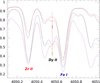 |
Fig. 5 Detection of the rare-earth element dysprosium (Dy) in the spectra of several library stars (from top to bottom for the Fe I line core; Sun, 70 Vir, α Boo, α Ari, μ Leo). Dysprosium’s name comes from greek dusprositos and means “hard to get at”. The singly-ionized Dy line at 4050.55 Å is indicated along with one Zr II and one Fe I line. |
6.3 Carbon 12C to 13C ratio
Meléndez et al. (2009) have shown that the Sun exhibits a depletion of refractory elements relative to volatile elements and related this to a cleansing effect during its rocky-planet formation. The engulfment of a close-orbiting planet during the RGB evolution may lead to the opposite effect, an overabundance of refractory elements, if fully transferred to the envelope of the host star. Various authors searched for signatures of such a replenishment in the Li abundances and its isotope ratio (e.g., Kumar et al. 2011) but also in 12C / 13C (e.g., Carlberg et al. 2012). Accurate C-isotope ratios require high-resolution and high S/N spectra while applicable only to stars cool enough to enable CN formation and with low vsini (e.g., Berdyugina & Savanov 1994). No conclusive statements on engulfing could be made so far from carbon abundances but it seems clear that initial protostellar Li abundances and 12C / 13C may be more diverse than originally thought (Carlberg et al. 2012). It is thus advisable also analyzing the carbon isotope ratio in benchmark RGB stars.
Figure 6 shows a comparison of the 800-nm region of three of the RGB stars in this paper (Arcturus, K1.5III; Hamal, K1IIIb; and Rasalas, K2III). The measurement of 12 C / 13C usually comes from fitting a small group of CN lines in the spectral region between 8001 and 8005 Å. There, one can see the isotope ratio even by eye, that is, by comparing the 8004 Å line depth, which is solely due to 12 CN, to the depth of the feature at 8004.7 Å, which is solely due to 13CN. CN identifications in the plot were taken from Carlberg et al. (2012). Spectra of this region are contaminated by telluric lines. We have demonstrated this in paper I for the solar spectra and for the solar twin 18 Sco. Figure 6 shows for comparison the Kurucz et al. (1984) telluric spectrum. For our plot the telluric spectrum was scaled and shifted to match the observed telluric spectrum of μ Leo (and can thus only be compared to the μ Leo spectrum in the plot in Fig. 6). It is self explaining that one should take its contamination into account when determining the carbon isotope ratio.
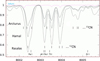 |
Fig. 6 Comparison of the 800-nm region of three RGB stars in this library; from top to bottom, Arcturus (α Boo, K1.5III), Hamal (α Ari, K1IIIb), Rasalas (μ Leo, K2III). The region contains many 12CN and 13 CN lines from which the 12C to 13 C ratio is derived. A telluric spectrum scaled to the Rasalas observation is shown on the top. |
6.4 Heavy elements
The formation of very heavy elements like uranium (Z = 92) or thorium (Z = 90) requires a process with rapid neutron capture, the so-called r-process, which is naturally happening during supernova explosions. The explosion ejects these elements into space where they are then available for the next generation of stars. Common uranium isotopes have half-life decay times of 108 to 109 years, and had been used to determine the age of the universe by observing ultra-metal-poor stars (Frebel et al. 2007). Gopka et al. (2007) identified Th II 5989.045 Å in the KPNO Arcturus spectrum from Hinkle et al. (2000). They followed this up by the identification of more such lines from the KPNO atlas (Gopka et al. 2013). The most widely used line is Th II 4019.129 Å. Together with the nearby neodymium line Nd II 4018.8 Å this line is used to form the chronometric ratio Th/Nd, first suggested by Butcher (1987) as an age indicator. However, there is no systematic identification of heavy-element lines in benchmark stars.
We have visually searched our library sample for the strong lines of U II at, for example 3859.57 Å and 4241.67 Å as well as Th IIat 4019.129 Å and 5989.045 Å, leaning on new oscillator strengths from Nilsson et al. (2002a,b). Some of these lines are indeed identified, for example the Th II-Nd II line pair at 5989 Å in giant stars like Arcturus, α Ari, or μ Leo or the U II transition at 4241-Å in ϵ Vir. Figure 7 is a comparison of above three targets with the Sun for the Th 5989-Å region. For many others there is only vague evidence due to blending. Note again that the solar spectrum in this plot was also taken with PEPSI in the same manner as the other stars. It shows a dominant telluric blend on the blue side of the expected Nd II line. Th II 5989.045 may be present in the solar spectrum with an upper limit at the <1 mÅ level.
In connection with chronometry, the s-process elements Ba and Sr (a.o.) are also key elements. The most prominent barium line is the one Ba II transition at 4554.02 Å. Other comparably weaker lines are 3891.78 Å and 4130.64 Å (see, e.g., Siqueira Mello et al. 2014).Strontium lines are comparably more prominent than U and Th, for example Sr II at 4077.72 Å or 5215.52 Å. The 4077-Å line is commonly used in the M-K system to classify cool, low-gravity, stellar atmospheres because of its density sensitivity (Gray & Garrison 1989). Our library spectra may be used to investigate spectral lines from heavy elements in greater detail than before.
 |
Fig. 7 Th II 5989.045-Å and Nd II 5989.378-Å lines in three RGB stars (full lines, from top to bottom in the Ti I line core; Arcturus, Hamal, Rasalas). The top spectrum shown as dots is a spectrum of the Sun. |
7 Summary
We present a library of high-resolution (on average ≈220 000), high-S/N optical spectra of a sample of 48 bright reference stars. The sample includes the northern Gaia benchmark stars and a few well-known M-K standards. Deep spectra are build by average combining individual exposures and reach S/N of many hundreds and, in some cases, even thousands. Continua are set by predetermining synthetic spectra that match the target classification. Continuum adjustments of several tens of per cent were necessary for wavelengths shorter than 400 nm. For all other wavelengths the differences in the continuum were always less than 1% and for wavelength regions with clear continuum visibility more like 0.2%.
A comparison with the KPNO Arcturus atlas revealed nearly perfect agreement with our library spectrum. At some wavelength regions the pixel-to-pixel differences are equal to or comparable to the photon noise level after both spectra were shifted in wavelength to the barycentric rest frame. We also found very weak Ca II H&K and Hα residual emission in Arcturus, thereby further strengthening earlier claims that it has a magnetic field and even an H&K activity cycle. The spectrum is still to be examined in detail whether the match also holds for other spectral lines. After all, the two spectra were taken 16 yr apart.
We identified several archival science cases possible to be followed up with the present data. Among these are the determination of global stellar parameters like effective temperature, gravity, metallicity, and elemental abundances. For a demonstration, we applied our spectrum synthesis code ParSES to a number of selected wavelength regions of 70 Vir (G4V-IV) and α Tau (K5III). The resulting values are summarized and compared with the literature in Table 3. These numbers are not intended to be the final verdict but shall just demonstrate the capabilities and the expected uncertainties.
Of particular interest are isotopic line ratios. The most asked for in the literature is the 6 Li to 7 Li ratio from the two Li doublets at 6708 Å. Its science cases range from rocky planet engulfment, internal stellar mixing and dredge-up mechanisms, to the primordial Li production rate. In our paper I on the Sun-as-a-star, we had analyzed this wavelength region of the Sun in detail and refer the reader to this paper. Another isotope ratio of general interest is 12 C / 13C. Its primary science case is the main chain of the CNO cycle in stellar evolution but also allows the quantification of dredge-up episodes on the RGB in more detail. Finally, elemental abundances of species “that are hard to get at” are made accessible, for example the rare-earth element dysprosium or the heavy elements uranium and thorium, just to name a few.
The reduced deep spectra can be downloaded in FITS format from our web page2. We also provide the deep 1D data prior to the final continuum normalization.
Log of individual spectra.
Continued.
Acknowledgements
We thank all engineers and technicians involved in PEPSI, in particular our Forschungstechnik team and its late EmilPopow who passed away much too early, but also Mark Wagner and John Little and his LBTO mountain crew. Our thanks also go to Christian Veillet, LBT director, and to Paul Gabor, VATT director, for their clever telescope scheduling. Walter Seifert, LSW Heidelberg, is warmly thanked for making some hours of his LUCI commissioning time available to us. It is also our pleasure to thank the German Federal Ministry (BMBF) for the year-long support through their Verbundforschung for LBT/PEPSI through grants 05AL2BA1/3 and 05A08BAC. Finally, the many telescope operators are thanked for their patience and even –partial– enthusiasm when we wanted to observe Sirius with a 12 m telescope. This research has made use of the SIMBAD database, operated at CDS, Strasbourg, France.
Appendix A: Detailed observing log
References
- Allende-Prieto, C. 2004, Astron. Nachr., 325, 604 [NASA ADS] [CrossRef] [Google Scholar]
- Allende-Prieto, C., Beers, T. C., Wilhelm, R., et al. 2006, ApJ, 636, 804 [NASA ADS] [CrossRef] [Google Scholar]
- Auriére, M. 2003, eds. J. Arnaud & N. Meunier, in EAS Pub. Ser. 9, 105 [CrossRef] [Google Scholar]
- Bagnulo, S., Jehin, E., Ledoux, C., et al. 2003, The Messenger, 114, 10 [NASA ADS] [Google Scholar]
- Berdyugina, S. V., & Savanov, I. S. 1994, Astron. Lett., 20, 639 [NASA ADS] [Google Scholar]
- Bernkopf J., Fiedler A., & Fuhrmann K. 2001, in Astrophysical Ages and Times Scales, eds. T. von Hippel, C. Simpson, & N. Manset (San Francisco: ASP), ASP Conf. Ser., 245, 207 [NASA ADS] [Google Scholar]
- Blanco-Cuaresma, S., Soubiran, C., Jofre, P., & Heiter, U. 2014, A&A, 566, A98 [NASA ADS] [CrossRef] [EDP Sciences] [Google Scholar]
- Bonanno, A., Benatti, S., Claudi, R., et al. 2008, ApJ, 676, 1248 [NASA ADS] [CrossRef] [Google Scholar]
- Brown, S. F., Gray, D. F., & Baliunas, S. L. 2008, ApJ, 679, 1531 [NASA ADS] [CrossRef] [Google Scholar]
- Butcher, H. 1987, Nature, 328, 127 [NASA ADS] [CrossRef] [Google Scholar]
- Carlberg, J. K., Cunha, K., Smith, V. V., & Majewski, S. R. 2012, ApJ, 757, 109 [NASA ADS] [CrossRef] [Google Scholar]
- Christensen-Dalsgaard, J., & Frandsen, S. 1983, Sol. Phys., 82, 469 [Google Scholar]
- Cowley, A., & Fraquelli, D. 1974, PASP, 86, 70 [NASA ADS] [CrossRef] [Google Scholar]
- Cowley, A. P., & Crawford, D. L. 1971, PASP, 83, 296 [NASA ADS] [CrossRef] [Google Scholar]
- Creevey, O. L., Thévenin, F., Berio, P., et al. 2015, A&A, 575, A26 [NASA ADS] [CrossRef] [EDP Sciences] [Google Scholar]
- Dall, T. H., Bruntt, H., Stello, D., & Strassmeier, K. G. 2010, A&A, 514, A25 [NASA ADS] [CrossRef] [EDP Sciences] [Google Scholar]
- Dekker, H., D’Odorico, S., Kaufer, A., Delabre, B., & Kotzlowski, H. 2000, SPIE, 4008, 534 [Google Scholar]
- Dragomir, D., Kane, S. R., Henry, G. W., et al. 2012, ApJ, 754, 37 [NASA ADS] [CrossRef] [Google Scholar]
- Fekel, F. C. 2003, PASP, 115, 807 [NASA ADS] [CrossRef] [Google Scholar]
- Frandsen, S., Carrier, F., Aerts, C., et al. 2002, A&A, 394, L5 [NASA ADS] [CrossRef] [EDP Sciences] [Google Scholar]
- Frebel, A., Christlieb, N., Norris, J. E., et al. 2007, ApJ, 660, L117 [NASA ADS] [CrossRef] [Google Scholar]
- Fuhrmann, K., Chini, R., Hoffmeister, V. H., et al. 2011, MNRAS, 411, 2311 [NASA ADS] [CrossRef] [Google Scholar]
- Gilmore, G., Randich, S., Asplund, M., et al. 2012, The Messenger, 147, 25 [NASA ADS] [Google Scholar]
- Gopka, V. F., Vasileva, S. V., Yushchenko, A. V., & Andrievsky, S. M. 2007, Odessa Astron. Publ., 20, 58 [NASA ADS] [Google Scholar]
- Gopka, V. F., Shavrina, A. V., Yushchenko, V. A., et al. 2013, Bull. of the Crimean Astrophys. Obs., 109, 41 [NASA ADS] [CrossRef] [Google Scholar]
- Gray, R. O., & Corbally, C. J. 1994, AJ, 107, 742 [NASA ADS] [CrossRef] [Google Scholar]
- Gray, R. O., & Garrison, R. F. 1989, ApJS, 69, 301 [NASA ADS] [CrossRef] [Google Scholar]
- Griffin, R. F. 1968, A photometric atlas of the spectrum of Arcturus, λ3600-8825Å (Cambridge: Cambridge Philosophical Society) [Google Scholar]
- Grundahl, F., Fredslund Andersen, M., Christensen-Dalsgaard, J., et al. 2017, ApJ, 836, 142 [NASA ADS] [CrossRef] [Google Scholar]
- Gustafsson, B. 2007, in Why Galaxies Care About AGB Stars: Their Importance as Actors and Probes, eds. F. Kerschbaum, C. Charbonnel, & R. F. Wing (San Francisco: ASP), ASP Conf. Ser., 378, 60 [NASA ADS] [Google Scholar]
- Hatzes, A. P., Zechmeister, M., Matthews, J., et al. 2012, A&A, 543, A98 [NASA ADS] [CrossRef] [EDP Sciences] [Google Scholar]
- Hatzes, A. P., Cochran, W. D., Endl, M., et al. 2015, A&A, 580, A31 [NASA ADS] [CrossRef] [EDP Sciences] [Google Scholar]
- Hawkins, K., Jofré, P., Heiter, U., et al. 2016, A&A, 592, A70 [NASA ADS] [CrossRef] [EDP Sciences] [Google Scholar]
- Heiter, U., Jofré, P., Gustafsson, B., et al. 2015, A&A, 582, A49 [NASA ADS] [CrossRef] [EDP Sciences] [PubMed] [Google Scholar]
- Hill, J., Green, R. F., Ashby, D. S., et al. 2012, SPIE, 8444-1 [Google Scholar]
- Hinkle, K., Wallace, L., Valenti, J., & Harmer, D. 2000, Visible and Near Infrared Atlas of the Arcturus Spectrum 3727–9300 Å (San Francisco: ASP) [Google Scholar]
- Hubrig, S., Plachinda, S. I., Hünsch, M., & Schröder, K. P. 1994, A&A, 291, 890 [NASA ADS] [Google Scholar]
- Ilyin, I. 2000, PhD Thesis, Univ. of Oulu [Google Scholar]
- Jofré, P., Heiter, U., Soubiran, C., et al. 2014, A&A, 564, A133 [NASA ADS] [CrossRef] [EDP Sciences] [Google Scholar]
- Jofré, P., Heiter, U., Soubiran, C., et al. 2015, A&A, 582, A81 [NASA ADS] [CrossRef] [EDP Sciences] [Google Scholar]
- Jovanovic, M., Weber, M., & Allende-Prieto, C. 2013, Publ. Astron. Obs. Belgrade, 92, 169 [NASA ADS] [Google Scholar]
- Keenan, P. C.,& Hynek, J. A. H. 1945, ApJ, 101, 265 [NASA ADS] [CrossRef] [Google Scholar]
- Keenan, P. C.,& McNeil, R. C. 1989, ApJS, 71, 245 [NASA ADS] [CrossRef] [Google Scholar]
- Kim, K. M., Mkrtichian, D. E., Lee, B. C., Han, I., & Hatzes, A. P. 2006, A&A, 454, 839 [NASA ADS] [CrossRef] [EDP Sciences] [Google Scholar]
- Kjeldsen, H., Bedding, T. R., Baldry, I. K., et al. 2003, AJ, 126, 1483 [NASA ADS] [CrossRef] [Google Scholar]
- Kumar, Y. B., Reddy, B. E., & Lambert, D. L. 2011, ApJ, 730, L12 [NASA ADS] [CrossRef] [Google Scholar]
- Kupka, F., et al. (VAMDC Collaboration) 2011, Baltic Astron., 20, 503 [NASA ADS] [Google Scholar]
- Kurucz, R. L., Furenlid, I., Brault, J., & Testerman, L. 1984, Solar Flux Atlas from 296 to 1300 nm, (Sunspot: National Solar Observatory) [Google Scholar]
- Lebzelter, T., Heiter, U., Abia, C., et al. 2012, A&A, 547, A108 [NASA ADS] [CrossRef] [EDP Sciences] [Google Scholar]
- Lee, B.-C., Han, I., Park, M.-G., et al. 2014, A&A, 566, A67 [NASA ADS] [CrossRef] [EDP Sciences] [Google Scholar]
- Lee, B. C., Han, I., Park, M.-G., et al. 2016, AJ, 151, 106 [NASA ADS] [CrossRef] [Google Scholar]
- Luck, R. E. 2014, AJ, 147, 137 [NASA ADS] [CrossRef] [Google Scholar]
- Luck, R. E., & Heiter, U. 2007, AJ, 133, 2464 [NASA ADS] [CrossRef] [Google Scholar]
- Mack, C. E. III, Strassmeier, K. G., Ilyin, I., Schuler, S. C., & Spada, F. 2018, A&A, 612, A46 [NASA ADS] [CrossRef] [EDP Sciences] [Google Scholar]
- Mayor, M., Pepe, F., Queloz, D., et al. 2003, The Messenger, 114, 20 [NASA ADS] [Google Scholar]
- McArthur, B. E., Benedict, F. G., Henry, G. W. et al. 2014, ApJ, 795, 41 [NASA ADS] [CrossRef] [Google Scholar]
- Meléndez, J., Asplund, M., Gustafsson, B., & Yong, D. 2009, ApJ, 704, L66 [NASA ADS] [CrossRef] [Google Scholar]
- Molaro, P., Esposito, M., Monai, S. et al. 2013, A&A, 560, A61 [NASA ADS] [CrossRef] [EDP Sciences] [Google Scholar]
- Morgan, W. W. 1972, AJ, 77, 35 [NASA ADS] [CrossRef] [Google Scholar]
- Morgan, W. W., & Roman, N. G. 1950, ApJ, 112, 362 [NASA ADS] [CrossRef] [Google Scholar]
- Nassau, J. J., & MacRae, D. A. 1949, ApJ, 110, 478 [NASA ADS] [CrossRef] [Google Scholar]
- Nilsson, H., Zang, Z. G., Lundberg, H., Johansson, S., & Nordström, B. 2002a, A&A, 382, 368 [NASA ADS] [CrossRef] [EDP Sciences] [Google Scholar]
- Nilsson, H., Ivarsson, S., Johansson, S., & Lundberg, H. 2002b, A&A, 381, 1090 [NASA ADS] [CrossRef] [EDP Sciences] [Google Scholar]
- Norlen, G. 1973, Phys. Scr., 8, 249 [NASA ADS] [CrossRef] [Google Scholar]
- Paletou, F., Böhm, T., Watson, V., & Trouilhet, J.-F. 2015, A&A, 573, A67 [NASA ADS] [CrossRef] [EDP Sciences] [Google Scholar]
- Palmer, B. A.,& Engleman, R. 1983, Atlas of the Thorium Spectrum (Los Alamos: National Laboratory) [Google Scholar]
- Probst, R. A., Wang, L., Doerr, H.-P. et al. 2015, New J. Phys., 17, 023048 [NASA ADS] [CrossRef] [Google Scholar]
- Reiners, A., Mrotzek, N., Lemke, U., Hinrichs, J., & Reinsch, K. 2016, A&A, 587, A65 [NASA ADS] [CrossRef] [EDP Sciences] [Google Scholar]
- Ryabchikova, T., Ryabtsev, A., Kochukhov, O., & Bagnulo, S. 2006, A&A, 456, 329 [NASA ADS] [CrossRef] [EDP Sciences] [Google Scholar]
- Sablowski, D. P., Weber, M., Woche, M., et al. 2016, SPIE, 99125H [Google Scholar]
- Sennhauser, C., & Berdyugina, S. V. 2011, A&A, 529, A100 [NASA ADS] [CrossRef] [EDP Sciences] [Google Scholar]
- Siqueira Mello, C., Hill, V., Barbuy, B., et al. 2014, A&A, 565, A93 [NASA ADS] [CrossRef] [EDP Sciences] [Google Scholar]
- Smiljanic, R., Korn, A. J., Bergemann, M., et al. 2014, A&A, 570, A122 [NASA ADS] [CrossRef] [EDP Sciences] [Google Scholar]
- Soubiran, C., Le Campion, J.-F., Cayrel de Strobel, G., & Caillo, A. 2010, A&A, 515, A111 [NASA ADS] [CrossRef] [EDP Sciences] [Google Scholar]
- Strassmeier, K. G. 2009, A&ARv, 17, 251 [NASA ADS] [CrossRef] [Google Scholar]
- Strassmeier, K. G., Weber, M., Granzer, T., & Järvinen, S. 2012, Astron. Nachr., 333, 663 [NASA ADS] [CrossRef] [Google Scholar]
- Strassmeier, K. G., Ilyin, I., Järvinen, A., et al. 2015, Astron. Nachr., 336, 324 [NASA ADS] [CrossRef] [Google Scholar]
- Strassmeier, K. G., Ilyin, I., & Steffen, M. 2018, A&A, 612, A44 [NASA ADS] [CrossRef] [EDP Sciences] [Google Scholar]
- Wallace, L., Hinkle, K. H., Livingston, W. C., & Davis, S. P. 2011, ApJS, 195, 6 [NASA ADS] [CrossRef] [Google Scholar]
- Wickliffe, M. E., Lawler, J. E., & Nave, G. 2000, J. Quant. Spectr. Rad. Transf., 66, 363 [NASA ADS] [CrossRef] [Google Scholar]
All Tables
Wavelength regions in Å that are affected by a bad-amplifier problem with the Blue CCD for the epoch November–December 2015.
All Figures
|
Fig. 1 Example spectrum of 70 Vir, spectral type G4 V–IV (x-axis is wavelength in Angstrom, y-axis is relative intensity). Top: full 5290-Å wavelength coverage. The other panels show magnifications of four selected wavelength regions. Top down: numerous Fe I lines around 4250 Å, the Mg I triplet at 5175 Å, the Li I 6708-Å region, and the 8004-Å line region commonly used for 12 C / 13C determination. |
| In the text | |
|
Fig. 2 Comparison of an average-combined spectrum and its individual exposures for β UMi (K4III). Thex-axes are wavelengths in Å. The 22 individual exposures are shown as lines, the average combined “deep spectrum” as dots. Panel a: a 0.8-Å section showing the 22 exposures of the K I 7699 Å line profile. The y-axis is relative intensity. No differences can be seen at this plot scale. Panel b: a zoom into a 0.08-Å subsection of the line core. The spacing of the dots represent the CCD pixel dispersion. Panel c: S/N per pixel in the K I line core for the same spectral window as in panel b. |
| In the text | |
|
Fig. 3 Examples for the typical S/N and spectral resolution of the library stars in this paper. Panel a: S/N of the deep spectrum of the G4 subgiant 70 Vir. The larger S/N in the very red wavelengths is mostly due to the larger number of individual spectra. Note that the local peaks in S/N are due to the wavelength overlap of the cross dispersers, which effectively doubles the number of pixels there. Panel b: spectral resolution for the focus achieved for the July 2016 run. |
| In the text | |
|
Fig. 4 Comparison of the deep PEPSI spectrum of Arcturus with the KPNO Arcturus atlas from Hinkle et al. (2000). Panel a: numerous CH lines centered around the Fe I/Ca I blend at 4308 Å that constitute the Fraunhofer G-band. The dots are the PEPSI spectrum and the line is the KPNO atlas. The match is nearly perfect. Panel b: three wavelength regions where chromospheric activity may be detected. Each panel shows the ratio spectrum PEPSI:KPNO (line around unity), the KPNO spectrum as a line, and the PEPSI spectrum as dots. From left to right, the core of the Ca II H line, Hα , and the Li I 6707.9-Å line region. |
| In the text | |
|
Fig. 5 Detection of the rare-earth element dysprosium (Dy) in the spectra of several library stars (from top to bottom for the Fe I line core; Sun, 70 Vir, α Boo, α Ari, μ Leo). Dysprosium’s name comes from greek dusprositos and means “hard to get at”. The singly-ionized Dy line at 4050.55 Å is indicated along with one Zr II and one Fe I line. |
| In the text | |
|
Fig. 6 Comparison of the 800-nm region of three RGB stars in this library; from top to bottom, Arcturus (α Boo, K1.5III), Hamal (α Ari, K1IIIb), Rasalas (μ Leo, K2III). The region contains many 12CN and 13 CN lines from which the 12C to 13 C ratio is derived. A telluric spectrum scaled to the Rasalas observation is shown on the top. |
| In the text | |
|
Fig. 7 Th II 5989.045-Å and Nd II 5989.378-Å lines in three RGB stars (full lines, from top to bottom in the Ti I line core; Arcturus, Hamal, Rasalas). The top spectrum shown as dots is a spectrum of the Sun. |
| In the text | |
Current usage metrics show cumulative count of Article Views (full-text article views including HTML views, PDF and ePub downloads, according to the available data) and Abstracts Views on Vision4Press platform.
Data correspond to usage on the plateform after 2015. The current usage metrics is available 48-96 hours after online publication and is updated daily on week days.
Initial download of the metrics may take a while.