| Issue |
A&A
Volume 610, February 2018
|
|
|---|---|---|
| Article Number | A42 | |
| Number of page(s) | 5 | |
| Section | The Sun | |
| DOI | https://doi.org/10.1051/0004-6361/201731490 | |
| Published online | 23 February 2018 | |
Energy spectra of carbon and oxygen with HELIOS E6
Radial gradients of anomalous cosmic ray oxygen within 1 AU
1
Christian-Albrechts-Universität zu Kiel,
Leibnizstr. 11,
24118
Kiel, Germany
e-mail: This email address is being protected from spambots. You need JavaScript enabled to view it.
2
Centre for Space Research, North-West-University,
Potchefstroom
2520, South Africa
Received:
3
July
2017
Accepted:
6
December
2017
Abstract
Context. Anomalous cosmic rays (ACRs) are well-suited to probe the transport conditions of cosmic rays in the inner heliosphere. We revisit the HELIOS data not only in view of the upcoming Solar Orbiter experiment but also to put constraints on particle transport models in order to provide new insight into the boundary conditions close to the Sun.
Aims. We present here the energy spectra of galactic cosmic ray (GCR) carbon and oxygen, as well as of ACR oxygen during solar quiet time periods between 1975 to 1977, utilizing both HELIOS spacecraft at distances between ~0.3 and 1 AU. The radial gradient (Gr ≈ 50%/AU) of 9–28.5 MeV ACR oxygen in the inner heliosphere is about three times larger than the one determined between 1 and 10 AU by utilizing the Pioneer 10 measurements.
Methods. The chemical composition as well as the energy spectra have been derived by applying the dE∕dx − E-method. In order to derive these values, special characteristics of the instrument have been taken into account.
Results. A good agreement of the GCR energy spectra of carbon and oxygen measured by the HELIOS E6 instrument between 0.3 and 1 AU and the Interplanetary Monitoring Platform (IMP) 8 at 1 AU was found. For ACR oxygen, we determined a radial gradient of about 50%/AU that is three times larger than the one between 7 and 14 AU, indicating a strong change in the inner heliosphere.
Key words: Sun: heliosphere / solar-terrestrial relations / cosmic rays
© ESO 2018
1 Introduction
The current paradigm of anomalous cosmic rays (ACRs) can be summarized as follows: interstellar neutrals that have been swept into the heliosphere are ionized in the heliosphere to become so-called pickup ions (PUIs; Fisk et al. 1974). Because of their high ionization potentials, He, N, O, and Ne are able to penetrate to within a few AU of the Sun before this happens (see Drews et al. 2016, and references therein). These singly ionized PUIs (Moebius et al. 1985) are subject to the Lorentz force and are therefore bound to the outward convecting heliospheric magnetic field. They become accelerated at the heliospheric termination shock (Pesses et al. 1981) and then diffuse into the heliosphere as mainly singly ionized energetic particles (Klecker et al. 1995). The crossings of the termination shock first by Voyager 1 (V1) and later by Voyager 2 (V2) have led to a new paradigm because the ACR spectra were not of the expected form (Decker et al. 2005). Several alternative acceleration models have been introduced since then (for a review, see Potgieter 2013, and references therein).
The interaction of energetic charged particles with the heliospheric magnetic field (HMF) reduces their intensities with decreasing distance to the Sun. Transport effects, in particular the adiabatic energy lose effect, yield the well known I(E) ∝ E proportionality for galactic cosmic rays (GCRs) at energies below about 100 MeV nucleon−1 (for a review, see Moraal 1993, and references therein).
Figure 1 displays the quiet-time energy spectra of hydrogen, helium, oxygen, nitrogen and carbon as measuredduring the 1970s solar minimum. While hydrogen shows the expected energy dependence with I(E) ∝ E1, all other elements show an upturn in the spectrum that is caused by the anomalous component that is most prominent for oxygen and nitrogen. Thus ACRs were first recognized by their different spectral shape at low energies (Hovestadt et al. 1973; Garcia-Munoz et al. 1973). The radial and latitudinal distribution of ACRs in the heliosphere can be determined by studying the evolution of the energy spectra of ions as a function of radial distance as well as latitude. The resulting radial and latitudinal gradients are therefore important to understand the transport of energetic particles in the heliosphere. Most studies concentrate on the gradients in the outer heliosphere using data from the pioneering space missions launched in the 1970s, such as Pioneer 10, Pioneer 11, V1, and V2,with the Interplanetary Monitoring Platform (IMP) 8 utilized as a baseline for their studies (see Fig. 1).
Webber et al. (1977) found a mean radial gradient of 20%/AU with a value of 25%/AU within 5 AU and 10%/AU from 5 to 10 AU, and of 5%/AU beyond 10 AU for anomalous oxygen. In a later publication, Webber et al. (1979) revised the values to 15%/AU. This value was used by Trattner et al. (1995, 1996) for the 1990s A > 0-solar magnetic epoch in order to determine the latitudinal gradients utilizing Ulysses and Solar Anomalous and Magnetospheric Particle Explorer (SAMPEX) measurements. However, Cummings et al. (1990, 1995) found the radial gradient to depend on the radial distance as r−0.96 and r−1.7 for an A < 0 and A > 0 solar magnetic epoch, respectively. Recent determinations of the radial gradient were performed by Cummings et al. (2009) for an A < 0-magnetic epoch utilizing the measurements from the low-energy telescopes aboard the Solar Terrestrial Relations Observatory (STEREO) A and B and Ulysses leading to a radial gradient of 45%/AU and 51%/AU at 4.5 to 15 and 7.3 to 15.6 MeV nucleon−1, respectively. Because of the strong dependence of the radial gradient on distance, larger radial gradients are expected in the inner than in the outer heliosphere. The only future measurements of ACR oxygen within the inner heliosphere will be performed by the Parker Solar Probe (Fox et al. 2016). However, recently we showed that the HELIOS E6 detector (Kunow 1981) is capable of separating the chemical composition up to neon (Marquardt et al. 2015). Therefore, we revisit here the energetic particle measurements gathered by the HELIOS experiment during the solar minimum from 1974 to 1977. In what follows, we apply the pulse height analysis developed by Marquardt et al. (2015) in order to determine reliable energy spectra for carbon and oxygen to infer the non-local differential radial gradient for ACR oxygen in the inner heliosphere between ~0.3 and 1 AU.
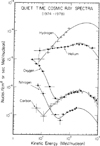 |
Fig. 1 Quiet-time energy spectra for the elements H, He, C, N, and O measured at 1 AU over the period from 1974 to 1978. We note the “anomalous” enhancements in the low-energy spectra of He, N, and O (Fig. 1.2 of Christian 1989). |
2 HELIOS and experiment 6 (E6)
HELIOS A and HELIOS B were launched on December 10, 1974 and January 15, 1976, respectively. The two almost identical space probes were sent into ecliptic orbits around the Sun. The orbital period around the Sun was 190 days for HELIOS A and 185 days for HELIOS B, and their perihelia were 0.3095 and 0.290 AU, respectively. The upper panels of Figs. 2 and 3 display the radial distance of HELIOS A and B from the launch of HELIOS A in 1974 to the end of 1978, receptively. Marked by the green and blue shaded regions are the close and far periods for which the spacecraft were within 0.45 AU and beyond 0.9 AU from the Sun. The lower panels of both figures indicate the hourly averaged count rate of 4 to 13 MeV nucleon−1 ions with z ≥ 2. Time periods that indicate intensity increases due to solar energetic particle events are indicated by the red shaded regions and have been omitted in our analysis.
The Kiel experiment, E6, has been described in detail by Kunow (1981). It is one of three particle detectors aboard HELIOS that allowed the study of energetic particles in the energy range from 1.3 MeV nucleon−1 to above 1000 MeV nucleon−1 for ions andfrom 0.3 to 8 MeV for electrons. Recently, Marquardt et al. (2015) showed that the instrument is capable of determining the chemical composition from hydrogen to neon in the energy range from a few to several tenths of a MeV nucleon−1.
The detector system is sketched in Fig. 4 and consists of five semi-conductor detectors of increasing thickness indicated in the figure; while the first two detectors, D1(A) and D2(B), are silicon-surface-barrier detectors with a thickness of 100 and 1000 μm, the other three are lithium drifted detectors with a thickness of 3000 μm. The first two (D1 and D2) are used for determining the lowest energy channels for the definition of the geometry factor for stopping particles (energy ranges below 51 MeV nucleon−1), as well as for discriminating between electrons and ions. Since the thickness of 100 μm does not allow us to measure minimum ionizing particles, electrons are separated from ions by the following trigger conditions:
-
no signal in the first detector → electron;
-
signal in the first detector → ion.
To avoid false identifications by these discrimination conditions, the first andsecond detectors are as close as possible to each other. Charged particles, which penetrate the fifth detector and the aluminum absorber beneath, are detected in the Sapphire-Cerenkov-detector. The Cerenkov-threshold for this material (n = 1.8) is Es =210 MeV nucleon−1. Because the Sapphire-Cerenkov-detector also delivers scintillation light, particles in the energy range above 51 MeV nucleon−1 are included in an integral channel.
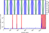 |
Fig. 2 Upper panel: radial distance of the HELIOS A space-probefrom the Sun. Indicated by the green and blue shaded regions are the close and far periods for which the spacecraft was within 0.3 and 0.45 AU, and 0.9 and 1 AU, respectively. Lower panel: count rate of Z ≥ 2 ions with energies from about 4 to 13 MeV nucleon−1 for helium.Shaded periods have been omitted in our analyses. |
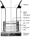 |
Fig. 4 Schematic of the HELIOS E6 (adapted from Marquardt et al. 2015). |
3 Data correction and analysis
The E6 particle telescope relies on the d E∕dx − E-method (see e.g. McDonald & Ludwig 1964). In order to interpret the measured data, a detailed understanding of the instrument is needed and can be obtained by modelling the physical processes inside the detector taking into account the instrument geometry as well as the environment (e.g. Heber et al. 2005; Marquardt et al. 2015). We need to correct for the so-called edge effects. Due to the decreasing charge collecting efficiency, from a certain radius outward the measured energy loss is spatially-dependent. This effect is particularly severe for the first two detectors, as described by Marquardt et al. (2015). Figure 5 displays the energy spectra of carbon (magenta symbols) and oxygen (black and red symbols) measured by HELIOS E6, binned in the same way as the energy spectra shown in Fig. 1. For oxygen we were able to restrict the time period under investigation to the periods when the spacecraft was beyond 0.9 AU. Due to the limited counting statistics, the whole time period, including periods when the spacecraft was close to the Sun, has to be used for carbon. The values for carbon (blue symbols) and oxygen (green symbols) from Fig. 1 have been added, indicating a reasonableagreement between the HELIOS and IMP observations. We note that for oxygen we utilized time periods when the spacecraft was beyond 0.9 AU. Due to the reduced statistics we need to take into account all periods for carbon, including the ones when HELIOS is within 0.9 AU. Therefore, we utilize only the HELIOS measurements in what follows. In order to determine radial gradients in the inner heliosphere, we divide the radial distances from the Sun into a set of measurements obtained during all far (1.0–0.9 AU) and close (0.45–0.3 AU) time periods (see Figs. 2 and 3). Since an upturn in the energy spectra is notable for energies below 30 MeV nucleon−1, oxygen ions below and above 30 MeV nucleon−1 are classified as ACRs and GCRs, respectively. For carbon, the total number of observed particles is insufficient to determine a radial gradient.
4 Results
Table 1 and Fig. 5 summarize the oxygen fluxes measured by HELIOS E6. The fluxes for oxygen are given in the same energy ranges as for IMP 8 (see Fig. 1). We use the fluxes during the far periods as a proxy for the 1 AU measurements.
Table 1 provides the oxygen fluxes in the energy range 9–28 MeV nucleon−1, similar to the energy range of 19–23.5 MeV nucleon−1 used by Webber et al. (1981). Assuming that temporal changes of the ACR oxygen flux are smaller than radial changes, we can calculate the corresponding radial gradient, Gr , as
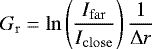 (1)
using Δr = 0.6 AU. These gradients are summarized in Table 2. The uncertainties given in the table take into account the statistical uncertainties only.
(1)
using Δr = 0.6 AU. These gradients are summarized in Table 2. The uncertainties given in the table take into account the statistical uncertainties only.
For GCR oxygen the ratio Ifar ∕Iclose is consistent with unity, thus implying a very small radial gradient. Webber et al. (1981) investigated the radial gradients of ACR oxygen measured from 1972 to 1980 by the Pioneer 10 and IMP spacecraft. They showed that the radial gradient had only slight variations from 1974 to 1977 when Pioneer 10 moved from about 7 AU to about 14 AU. In their Fig. 2 they give a mean value of Gr =15 %/AU. The upper panel of Fig. 6 shows the Pioneer 10 to IMP ratio in the energy range between 9 and 28.5 MeV nucleon−1 as a function of radial distance for the solar minimum period of solar cycle 22. The data are taken from (Webber et al. 1981) Fig. 2, and indicated on the figure by magenta triangles. Inaddition, the HELIOS close to far ratio, at ~0.38 AU, obtained during the time span from 1975 to mid 1977, is included as the black square. The middle and lower panels of the figure show the radial gradient, calculated by using Eq. (1), as a function of time and distance. From this figure itis evident that a strong increase with decreasing distance in the radial gradient must occur in the inner heliosphere within 2 AU.
The red triangles in the lower panel of Fig. 6 show the results of the computations described by Strauss & Potgieter (2010). Whereas the computations show an increase of the ACR-oxygen gradient from 14 AU inwards, peaking between 2 and 3 AU, the Pioneer 10 measurements show a nearly constant radial gradient of about 10 to 15%/AU from 3 to 14 AU, but the gradient then follows the predicted trend beyond 10 AU. However, the HELIOS measurements indicate a larger radial gradient that is in good agreement with the maximum gradient of the model, although much closer to the Sun. Pioneer 10 measurements between 7 to 14 AU coincide with the time of the HELIOS observations.
The results shown in Fig. 6 therefore indicate that ACR oxygen can easily penetrate into the inner heliosphere within 0.6 AU. The fact that the model and observations agree beyond ~ 10 AU is indeed encouraging, even more so that the maximum value of the gradient,  %/AU, also seems to be consistent with the model prediction.
The quantitative differences between the model and observationsshould, however, be investigated in detail in future. Reasons for the disagreement may include: (1) Since the Pioneer observations within 7 AU were obtained during a different phase of the solar cycle, these measurements may be influenced by temporal effects, while the computations are solutions of a steady-state model. (2) Near the Sun, and especially within 1 AU, the inner boundary condition assumed in the model may influence the calculated gradient (see also the discussion by Strauss & Potgieter 2010). (3) The assumed Parker (1965) transport equation might not be valid closer to the Sun as magnetic focussing can lead to an anisotropic ACR distribution. (4) Ultimately, the computed gradients depend on the diffusion and drift coefficients as assumed in the model. They, on their part, are based on the underlaying assumed turbulence, diffusion, and drift theories, which may need to be refined for ACR oxygen by observance of the new measurements presented here.
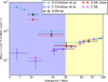 |
Fig. 5 Energy spectra of carbon and oxygen measured by the E6 in comparison with the data taken from Fig. 1. |
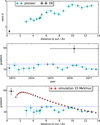 |
Fig. 6 Upperpanel: radial dependence of the ACR oxygen flux ratio in the energy range between 9 and 23.5 MeV nucleon−1 . Data beyond 1 AU are taken from Webber et al. (1981). Middle and lower panels: temporal and radial variation of the radial gradient. The red symbols show the computations from the modelling of Strauss & Potgieter (2010). |
5 Summary and conclusion
Marquardt et al. (2015) showed that the HELIOS E6 experiment is well suited for measuring the chemical composition of particles from carbon to neon. Here, we determined the quiet-time spectrum of carbon and oxygen in the energy range from 9 MeV nucleon−1 to above 80 MeV nucleon−1. A good agreement between the HELIOS and the IMP measurements, as reported by Christian (1989), was found. In order to compute the radial gradient in the inner heliosphere, the data set was divided into a period when the spacecraft was within 0.45 AU (Iclose) and another period with distances greater than 0.9 AU (Ifar ).
For GCR oxygen with energies between 30 and 80 MeV nucleon−1, the ratio between the fluxes measured close to and far from the Sun is consistent with 1.0 ± 0.1, indicating no significant radial gradient. However, for ACR oxygen, a significant radial gradient of  %/AU and
  %/AU was found for 9 to 13 and 13 to 28 MeV nucleon−1. By assuming a spectral shape of I(E) ∝ E1 for the GCRs and subtracting this GCR contribution from the flux in the 13 to 28 MeV nucleon−1 range, the gradient increases to Gr = 40%/AU. However, due to the uncertainties of this method a detailed error estimation is beyond the scope of this work.
When using the whole energy range from 9 to 28.5 MeV nucleon−1, we find  %/AU. This energy range was used also by Webber et al. (1981) to determine the radial dependence of Gr beyond 1 AU. The radial gradient that we report here is about three times larger than the one determined between 1 and 10 AU by utilizing the Pioneer 10 measurements.
Comparing results from these Pioneer 10 measurements to HELIOS results, we find that the radial gradient of ACR oxygen significantly increases within the first 2 AU from the Sun. Evidently, ACR oxygen, with a rigidity much larger than GCR oxygen, may penetrate the heliosphere to come very close to the Sun, exhibiting in the process a very steep gradient. Future information to validate our results will come from the Parker Solar Probe.
Acknowledgments
The work was partly carried out within the framework of the bilateral BMBF-NRF-project “Astrohel” (01DG15009) as supported by the Bundesministerium für Bildung und Forschung (BMBF) and the South African National Research Foundation (NRF).
References
- Christian, E. R. 1989, PhD thesis, California Institute of Technology, Pasadena [Google Scholar]
- Cummings, C. A., Mewaldt, A. R., Stone, C. E., & Webber, R. W. 1990, Int. Cosmic Ray Conf., 6, 206 [NASA ADS] [Google Scholar]
- Cummings, A. C., Mewaldt, R. A., Blake, J. B., et al. 1995, Geophys. Res. Lett., 22, 341 [NASA ADS] [CrossRef] [Google Scholar]
- Cummings, A. C., Tranquille, C., Marsden, R. G., Mewaldt, R. A., & Stone, E. C. 2009, Geophys. Res. Lett., 36, L18103 [NASA ADS] [CrossRef] [Google Scholar]
- Decker, R. B., Krimigis, S. M., Roelof, E. C., et al. 2005, Science, 309, 2020 [NASA ADS] [CrossRef] [PubMed] [Google Scholar]
- Drews, C., Berger, L., Taut, A., & Wimmer-Schweingruber, R. F. 2016, A&A,588, A12 [NASA ADS] [CrossRef] [EDP Sciences] [Google Scholar]
- Fisk, L. A., Kozlovsky, B., & Ramaty, R. 1974, ApJ, 190, L35 [NASA ADS] [CrossRef] [Google Scholar]
- Fox, N. J., Velli, M. C., Bale, S. D., et al. 2016, Space Sci. Rev., 204, 7 [NASA ADS] [CrossRef] [Google Scholar]
- Garcia-Munoz, M., Mason, G. M., & Simpson, J. A. 1973, ApJ, 182, L81 [NASA ADS] [CrossRef] [Google Scholar]
- Heber, B., Kopp, A., Fichtner, H., & Ferreira, S. E. S. 2005, Adv. Space Res., 35, 605 [NASA ADS] [CrossRef] [Google Scholar]
- Hovestadt, D., Vollmer, O., Gloeckler, G., & Fan, C. Y. 1973, Int. Cosmic Ray Conf., 2, 1498 [NASA ADS] [Google Scholar]
- Klecker, B., McNab, M. C., Blake, J. B., et al. 1995, ApJ, 442, L69 [NASA ADS] [CrossRef] [Google Scholar]
- Kunow, H. 1981, Cosmis ray experiment on board the solar probes Helios-1 and 2 (experiment no. 6), Tech. Rep. [Google Scholar]
- Marquardt, J., Heber, B., Hörlöck, M., Kühl, P., & Wimmer-Schweingruber, R. F. 2015, J. Phys. Conf. Ser., 632, 012016 [CrossRef] [Google Scholar]
- McDonald, F. B., & Ludwig, G. H. 1964, Phys. Rev. Lett., 13, 783 [NASA ADS] [CrossRef] [Google Scholar]
- Moebius, E., Hovestadt, D., Klecker, B., Scholer, M., & Gloeckler, G. 1985, Nature, 318, 426 [NASA ADS] [CrossRef] [Google Scholar]
- Moraal, H. 1993, Nucl. Phys. B Proc. Suppl., 33, 161 [NASA ADS] [CrossRef] [Google Scholar]
- Parker, E. N. 1965, Planet. Space Sci., 13, 9 [Google Scholar]
- Pesses, M. E., Eichler, D., & Jokipii, J. R. 1981, ApJ, 246, L85 [NASA ADS] [CrossRef] [Google Scholar]
- Potgieter, M. S. 2013, Liv. Rev. Sol. Phys., 10, 3 [Google Scholar]
- Strauss, R. D., & Potgieter, M. S. 2010, J. Geophys. Res. (Space Phys.), 115, A12111 [NASA ADS] [CrossRef] [Google Scholar]
- Trattner, K. J., Marsden, R. G., Sanderson, T. R., et al. 1995, Geophys. Res. Lett., 22, 337 [NASA ADS] [CrossRef] [Google Scholar]
- Trattner, K. J., Marsden, R. G., Bothmer, V., et al. 1996, A&A, 316, 519 [NASA ADS] [Google Scholar]
- Webber, W. R., McDonald, F. B., & Trainor, J. H. 1977, Int. Cosmic Ray Conf., 3, 233 [NASA ADS] [Google Scholar]
- Webber, W. R., McDonald, F. B., Trainor, J. H., & von Rosenvinge, T. T. 1979, Int. Cosmic Ray Conf., 5, 353 [NASA ADS] [Google Scholar]
- Webber, W. R., McDonald, F. B., von Rosenvinge, T. T., & Mewaldt, R. A. 1981, Int. Cosmic Ray Conf., 10, 92 [NASA ADS] [Google Scholar]
All Tables
All Figures
|
Fig. 1 Quiet-time energy spectra for the elements H, He, C, N, and O measured at 1 AU over the period from 1974 to 1978. We note the “anomalous” enhancements in the low-energy spectra of He, N, and O (Fig. 1.2 of Christian 1989). |
| In the text | |
|
Fig. 2 Upper panel: radial distance of the HELIOS A space-probefrom the Sun. Indicated by the green and blue shaded regions are the close and far periods for which the spacecraft was within 0.3 and 0.45 AU, and 0.9 and 1 AU, respectively. Lower panel: count rate of Z ≥ 2 ions with energies from about 4 to 13 MeV nucleon−1 for helium.Shaded periods have been omitted in our analyses. |
| In the text | |
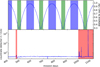 |
Fig. 3 Similar to Fig. 2, but for HELIOS 2. |
| In the text | |
|
Fig. 4 Schematic of the HELIOS E6 (adapted from Marquardt et al. 2015). |
| In the text | |
|
Fig. 5 Energy spectra of carbon and oxygen measured by the E6 in comparison with the data taken from Fig. 1. |
| In the text | |
|
Fig. 6 Upperpanel: radial dependence of the ACR oxygen flux ratio in the energy range between 9 and 23.5 MeV nucleon−1 . Data beyond 1 AU are taken from Webber et al. (1981). Middle and lower panels: temporal and radial variation of the radial gradient. The red symbols show the computations from the modelling of Strauss & Potgieter (2010). |
| In the text | |
Current usage metrics show cumulative count of Article Views (full-text article views including HTML views, PDF and ePub downloads, according to the available data) and Abstracts Views on Vision4Press platform.
Data correspond to usage on the plateform after 2015. The current usage metrics is available 48-96 hours after online publication and is updated daily on week days.
Initial download of the metrics may take a while.