© ESO 2018

1 Introduction

Models of solar flares and coronal heating mechanisms require the build-up and storage of magnetic energy in the coronal magnetic field. This build-up of magnetic energy is frequently modelled by imposing slow photospheric motions that gently stress the coronal field. The common assumption, valid when the driving velocities are very low compared with the coronal Alfvén speed, is that the magnetic field will simply pass through a sequence of equilibrium states until the critical conditions, for either an instability or non-equilibrium, are reached and the magnetic energy is subsequently released.

Ideally, one would like to model this evolution through the full time-dependent non-linear magnetohydrodynamic (MHD) equations. This requires the adoption of a computational approach, but at present, limitations on resources make the slow evolution over long times difficult to complete. Instead, a variety of approximate approaches that treat the coronal magnetic field in a simplified way have been used. These make different assumptions in order to achieve tractability, and it is important to understand how these approaches compare with each other and, especially, how they compare with a full MHD treatment. This has not been carried out before and is the purpose of this paper.

To this end, we consider an idealised problem of the shearing of an initially uniform magnetic field in a straightened coronal loop (with the photosphere modelled as two parallel boundaries). Four approximate methods are used, two that consider quasi-static evolution and calculate equilibrium fields and two that consider the time evolution of the field. We note that in the former category, one can calculate a sequence of equilibria in response to footpoint motions, but the intermediate time evolution is lost. The success of these approximate models are benchmarked against solutions of the full MHD equations using the Lare computational method Arber et al. (2001). The first quasi-static methodology considered is the relaxation or magneto-frictional method Yang et al. (1986); Yang (1989, 1990, 1992); Klimchuk & Sturrock (1992), which – together with a flux transport model Mackay & van Ballegooijen (2006a,b) – can be used to track the long time evolution of the force-free, coronal magnetic field from days to years. How the field reaches equilibrium is not considered in this approach, but the relaxed state, for the given time evolution of the photospheric magnetic field, is the main goal. This is discussed in Sect. 2.3. If there is no equilibrium, for example if a coronal mass ejection (CME) occurs, the relaxation code fails to converge.

The second method is based on the well-known idea that 2D equilibria satisfy the Grad-Shafranov equation for the magnetic flux function, A (see Sect. 2.4), but in general it is difficult to determine, for specified footpoint displacements, the unknown functional dependencies of the gas pressure and the shear component of the magnetic field on A. However, Lothian & Hood (1989) and Browning & Hood (1989) used the fact that there is a narrow boundary layer through which the various variables rapidly change from their boundary values to coronal values and that the coronal values only depend on one coordinate. Thus, the 2D approach can be reduced to a 1D problem (in the case when the length of the coronal loop is much greater than the scale of variation of the footpoint motions).

With time-dependent methods, the simplest and most common way to study the evolution is to linearise the MHD equations about a simple initial uniform initial state, as described by Rosner & Knobloch (1982). While linearised MHD is straightforward, the possible complexities for this class of problem can be demonstrated by taking the expansion procedure to a higher order. Thus, we can study weakly non-linear effects, due to the non-linear back reaction of the linear solution. The solutions, described in detail in Sect. 2.5 and in the appendix, also reveal features that help to justify the use of the 1D solution mentioned above.

Finally, time-dependent non-linear evolution can also be described by the reduced MHD (RMHD) equations. By eliminating the fast magnetoacoustic waves and utilising the difference in horizontal and parallel length scales, a set of simpler equations can be obtained. The method of RMHD was introduced for laboratory fusion plasma by e.g. Kadomtsev & Pogutse (1974); Strauss (1976); Zank & Matthaeus (1992), and used for coronal plasmas by e.g. Scheper & Hassam (1999) and Rappazzo et al. (2010, 2013). A recent review by Oughton et al. (2017) discusses the validity of the RMHD equations.

There are a few similar investigations for other situations, for example Pagano et al. (2013), who have compared the relaxation method with an MHD simulation for the onset of a CME; Dmitruk et al. (2005), who compare RMHD with MHD for the case of turbulence; and Schrijver et al. (2006), who test force-free extrapolations against a known solution. Examples of footpoint driven simulations include Murawski & Goossens (1994); Meyer et al. (2011, 2012, 2013).

Section 2 describes the simple footpoint shearing experiment, and outlines the details of the four approximate models we examine. Section 3 presents a comparison between these models and benchmarks them against solutions to the full MHD equations. We find that some methods perform quite well, even when their basic assumptions are not necessarily satisfied. A discussion of the results and possible future benchmarking exercises are presented in Sect. 4.

2 MHD equations and solution methods

2.1 MHD: basic equations

The time evolution of our simple experiment, which is outlined below, is determined by solving the viscous, ideal MHD equations. The full set of equations are expressed as $$\begin{array}{l}\rho \frac{\partial \overrightarrow{v}}{\partial t}+\rho (\overrightarrow{v}\cdot \nabla )\overrightarrow{v}=-\nabla p+\overrightarrow{j}\times \overrightarrow{B}+\nabla \cdot \overrightarrow{S},\\ \frac{\partial \rho }{\partial t}+\nabla \cdot (\rho \overrightarrow{v})=0,\\ \frac{\partial \overrightarrow{B}}{\partial t}=\nabla \times (\overrightarrow{v}\times \overrightarrow{B}),\\ \frac{\partial }{\partial t}\left(\frac{p}{\gamma -1}\right)+\overrightarrow{v}\cdot \nabla \left(\frac{p}{\gamma -1}\right)=-\frac{\gamma p}{\gamma -1}\nabla \cdot \overrightarrow{v}+{ϵ}_{ij}{S}_{ij},\end{array}$$

together with $$j=\frac{\nabla \times B}{\mu }\text{ and }\nabla \cdot B=0,$$

where v is the plasma velocity, ρ the mass density, p the gas pressure, B the magnetic field, and j the current density. Gravity is neglected. The viscous stress tensor is given by $$S_{ij}=2\rho \nu \left({ϵ}_{ij}-\frac{1}{3}{\delta }_{ij}\nabla \cdot v\right),$$

where ν is the viscosity and the strain rate is $${ϵ}_{ij}=\frac{1}{2}\left(\frac{\partial v_i}{\partial x_j}+\frac{\partial v_j}{\partial x_i}\right)\cdot$$

Equations (1)–(4) conserve the total energy, E = $\frac{1}{2}\rho v^2+\frac{B^2}{2\mu }+\frac{p}{\gamma -1}$, so that the dissipation of kinetic energy must go either into an increase in magnetic energy or an increase in internal energy (i.e. the gas pressure) defined as $e=\frac{p}{\gamma -1}$. The form of the viscous stress tensor does not include the anisotropies introduced by the magnetic field. However, for this experiment the main role of the viscosity is to damp out the waves generated by the boundary motions and to allow the field and plasma to evolve through sequences of equilibrium states so its exact form is not essential. Resistivity is not included as, in general, it decreases the magnetic energy. It has been confirmed that numerical resistivity is negligible as the energy injected at the boundaries equals the energy in the system within ~ 1%. The aim is to follow a sequence of magnetostatic equilibria.

It is normal to express the variables in the MHD equations in terms of non-dimensional ones and look for dimensionless parameters in the system. Then, it may be possible to use the fact that these parameters are either very large or very small to determine approximate solutions. Hence, we define a length scale R, a density ρ₀, and a magnetic field strength B₀. The dimensionless speed is the Alfvén speed, V_A = B₀/$\sqrt{\mu {\rho }_0}$, and time isexpressed in terms of the Alfvén travel time, t₀ = R∕V_A. Hence, we set $$\begin{array}{l}\left(x,y,z\right)=R\left(\tilde{x},\tilde{y},\tilde{z}\right),t=\frac{R}{V_{\text{A}}}\tilde{t},B=B_0\tilde{B},\\ p=\frac{B_0^2}{\mu }\tilde{p},v=V_{\text{A}}\tilde{v},\rho ={\rho }_0\tilde{\rho }.\end{array}$$(5)

Substituting these expressions into Eqs. (1)–(4) and dropping the tildes, the equations remain exactly the same, except that μ = 1 and ν is a non-dimensionless viscosity that is the inverse of the Reynolds number. For the values R = 2 × 10⁷ m, ρ₀ = 1.67 × 10⁻¹² kg m⁻³, and B₀ = 10⁻³ tesla, the Alfvén speed is V_A = 690 km s⁻¹ and the Alfvén travel time is t₀ = 29 s.

2.2 Experiment description

Consider a computational box − l ≤ x ≤ l and − L ≤ y ≤ L, and an initial uniform magnetic field B = B₀ŷ, uniform density ρ₀, and uniform pressure p₀. This can be thought of as a coronal loop of length 2L and width 2l with a dimensionless plasma β equal to 2p∕B², and we will use the term “loop” though the results are generic. In our dimensionless variables, B₀ = 1, ρ₀ = 1, and p₀ is a constant related to the initial plasma beta, β₀, by β₀ = 2p₀ and initial internal energy by $e_0=\frac{p_0}{\gamma -1}$.

Now impose a shearing velocity in the z direction at the two photospheric ends (y = ±L); z is chosen to be an ignorable coordinate so that the MHD equations will reduce to the appropriate 2.5D form. For the driving motions, we select $$v_z(x,\pm L,t)=\pm F(t)\sin kx,$$(6)

where k = π∕l and v_z (±l, y, t) = 0. The time variation of the shearing velocity is taken as $$F(t)=\frac{V_0}{2}\left\{\tanh \left(\frac{t-t_1}{{\tau }_0}\right)+1\right\},$$(7)

where t₁ > τ₀ is the switch-on time. We use t₁ = 6 and τ₀ = 2. If the parameter τ₀ is small, then F(t) can be approximated by $$F(t)=\{\begin{array}{cc}0,& t<t_1,\\ V_0,& t_1\le t.\end{array}$$(8)

We can also switch the driving off by using a similar function to ramp down the velocity.

This form of the velocity on the boundary will cause the photospheric footpoints to be displaced by a distance d(x) = Dsinkx. The maximum footpoint displacement, D, can be calculated by integrating the velocity amplitude in time as $$D={\displaystyle {\int }_0^{t}F}(t)\text{d}t=\frac{V_0\tau }{2}\left(\log \left\{\cosh \left(\frac{t-t_1}{\tau }\right)\right\}+\frac{t}{\tau }\right)\approx V_0(t-t_1),$$(9)

for times greater than t₁. Thus, we have three distinct lengths in this problem: the half-length of the loop, L; the half-width of the loop, l; and the photospheric footpoint displacement, d(x), from its initial position. In all cases, we take L = 3 and l= 0.3 so that l∕L = 0.1 ≪ 1. However, we allow D∕L to vary from low to high values.

Next, we consider the various speeds in our system. These are the Alfvén speed, V_A; sound speed, $c_{\text{s}}=\sqrt{\gamma p_0/{\rho }_0}$ (γ = 5∕3 is the ratio of specific heats); the speed of the driving motions at the photospheric ends, V₀; and a diffusion speed, V_visc = ν∕l, based on the horizontal lengthscales.Typically we take ν = 10⁻³ so that V_visc ≈ 3 × 10⁻³. A smaller value of ν could be used, but a value that is too small results in numerical diffusion being more important than the specified value. In order to pass through sequences of equilibria, we require $$V_{\text{visc}}\ll V_0\ll c_{\text{s}}.$$(10)

The driving speed is also slow and sub-Alfvénic if V₀ ≪ 1 from Eq. (5). Accordingly, we choose V₀ as 0.02. Equation (10) then requires that the pressure should be higher than a minimum value of p₀ ≫ 2.4 × 10⁻⁴. We consider the range 10⁻³ < p₀ < 1.0. Equivalently, this can be written in terms of the initial plasma β₀ as 2 × 10⁻³ < β₀ < 2.0 or in terms of the initial internal energy as $\frac{3\times {10}^{-3}}{2}<e_0<\frac{3}{2}$.

2.3 Relaxation

Magneto-frictional relaxation methods solve the induction equation with the velocity given by the unbalanced Lorentz force (see Mackay& van Ballegooijen 2006a,b). This approach has had great success in modelling the long-term evolution of the global coronal field and in predicting the onset of CMEs.

To ensure that ∇⋅B = 0, we express the magnetic field in terms of a vector magnetic potential, A = (A_x(x, y), A_y(x, y), A(x, y)), so that $$B=\nabla \times A=\left(\frac{\partial A}{\partial y},-\frac{\partial A}{\partial x},\frac{\partial A_y}{\partial x}-\frac{\partial A_x}{\partial y}\right)\cdot$$(11)

The equations to be solved are $$\begin{array}{l}v=\lambda \frac{j\times B}{B^2},\hfill \\ \frac{\partial A}{\partial t}=v\times B,\hfill \end{array}$$

where λ = 0.3 is the magneto-frictional constant (see Mackay & van Ballegooijen 2006a,b, for details).

The time evolution is not physically realistic and is a function of the footpoint displacement but leads to an end state in which the magnetic field has relaxed to a force-free equilibrium, with the imposed B_z from our shearing displacement. Hence, the magnetic energy can be calculated for a given displacement D. However, since the velocity is not a realistic quantity the kinetic energy cannot be calculated. Once the relaxation process is complete and since the resulting equilibrium is independent of the coordinate z, the z component of A(x, y) is a flux function and the relaxed z component of the magnetic field, B_z = ∂A_y∕∂x − ∂A_x∕∂y, will be a function of the flux function A(x, y), i.e. B_z = B_z(A). The boundary conditions for the vector potential are $$A_x(x,\pm L)=\mp B_{0}D\sin (\pi x/l)\text{ and }A(x,\pm L)=-B_{0}x.$$(14)

Without loss of generality, the gauge function is chosen so that A_y (x, ±L) = 0 and, once the field has relaxed, this implies that A_y(x, y) = 0. We select a physical time t, and use Eq. (9) to determine the maximum footpoint displacement D. We note that while solving the Grad-Shafranov equation, Eq. (15) below for a final force-free equilibrium state involves only A, the evolution towards such an equilibrium, described by Eq. (13), requires calculation of A_x as well.

Given a value of D, the magneto-frictional method of Mackay & van Ballegooijen (2006a,b) determines the equilibrium force-free field. For illustration only, we choose D = 3.0 (equivalent to t = 156) so that D is equal to the half-length L.The relaxed state for B_y is shown in Fig. 1. A more detailed comparison with the other methods is presented in Sect. 3.

There are two important points. Firstly, there are sharp boundary layers at the photospheric ends of the field; in this case they have a width of y∕R = 0.1, which equals l∕L. Different values of this ratio,0.05, 0.2, and 0.3 have been tested and it is concluded that the width of these boundary layers is controlled by the width-to-length ratio, l∕L. This is also given by the linearised MHD method in Sect. 2.5. This shows that B_y rapidly changes from the imposed constant boundary value of B₀ over a short distance that is comparable to the half-width, l. Hence, the derivative with respect to y of not just B_y but of several variables are large in the boundary layers. The width of the boundary layer is not dependent on the value of D∕L, and we use this in the next section when discussing the 1D approach.

Secondly, in the middle of the layer, away from the boundaries, B_y is almost independentof y, but it does vary with x as cos(2kx) when D∕L is low. Thus, although the dominant y component of the field started out uniform, when the footpoint displacement is comparable to the length L, the variations in B_y are of the order of 10%. Thus, the magneto-frictional method predicts what will turn out to be a generic property of relaxed states.

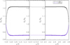Fig. 1 By∕B0 as a functionof y for the loop axes x = 0 (upper) and x = l∕2 (lower) using the magneto-frictional relaxation method. The horizontal scale is expanded at the two ends to illustrate the resolved boundary layers at y = ±L and compressed in the middle to demonstrate that there is no variation with y there.

2.4 One-dimensional equilibrium

When l∕L ≪ 1 a simple estimate of the final equilibrium state is possible, even when the footpoint displacement D is larger than the half-length L, i.e. D∕L ≥ 1, by solving the 1D form of the Grad-Shafranov equation. Following the approach of Lothian & Hood (1989); Browning & Hood (1989), and Mellor et al. (2005), we can use the fact that the 2D equilibrium can be expressed in terms of the flux function A(x, y), which satisfies the Grad-Shafranov equation: $${\nabla }^{2}A+\frac{\text{d}}{\text{d}A}\left(\mu p(A)+\frac{1}{2}{B}_z^2(A)\right)=0.$$(15)

The pressure is a function of A, which is determined by the energy equation, and B_z is determined by the shearing introduced by the footpoint displacement. For shearing motions defined in Eqs. (6)–(9), the photospheric footpoint displacement is given by integrating a fieldline from its initial position, (x₀, y₀), to its final one at (x, y). Hence, it is a function of the flux function and is given by $$\begin{array}{ll}D(A(x,L))\hfill & ={\displaystyle {\int }_{y=0}^{y=+L}{\left(\frac{B_z(A)}{B_y}\right)}_{A=\text{const}}}\text{d}y\hfill \\ \hfill & =B_z(A){\displaystyle {\int }_{y=0}^{y=+L}{\left(\frac{1}{-\partial A/\partial x}\right)}_{A=\text{const}}}\text{d}y.\hfill \end{array}$$(16)

As shown inthe above papers and from the magneto-frictional relaxation results, away from the boundaries we can ignore the boundary layers and assume that the field lines are essentially straight over most of the loop. A value of l∕L ≪ 1 is always assumed. Away from the boundary layers A is independentof y and this implies that the integrand is independent of y. Therefore, we can determine B_z(A) in terms of the footpoint displacement. Following Mellor et al. (2005), we have $$B_z(A)=-\frac{\text{d}(A)}{L}\frac{\text{d}A}{\text{d}x}\cdot$$(17)

For the shearing motion used above, we have at y = L that d(A) = V₀(t − t₁)sinkx, where k = π∕l and A(x, L) = −B₀x. Hence, d(A) = −V₀(t − t₁)sin(kx) = −Dsin(kA∕B₀), where D = V₀(t − t₁) is the maximum footpoint displacement.

The simple 1D approximation can be modified to include the gas pressure. Conservation of flux and mass between any two fieldlines implies that $$\frac{B_y}{\rho }=\frac{B_0}{{\rho }_0},$$(18)

where B₀ and ρ₀ are the initial unsheared values. Next, if the effect of viscous heating is small, the entropy remains constant between any two fieldlines so that $$\frac{p}{{\rho }^{\gamma }}=\frac{p_0}{{\rho }_0^{\gamma }}\cdot$$(19)

Rearranging the last two equations gives the pressure in terms of B_y as $$p=\frac{p_0}{B_0^{\gamma }}{B}_y^{\gamma }=\frac{p_0}{B_0^{\gamma }}{\left(-\frac{\text{d}A}{\text{d}x}\right)}^{\gamma },$$(20)

where − ∂A∕∂x > 0. Hence, the Grad-Shafranov equations reduces to a 1D pressure balance equation of the form $$\frac{\text{d}}{\text{d}x}\left(B_y^2+{\left(\frac{D}{L}\right)}^2{\sin }^2(kA/B_0)B_y^2+2p\right)=0.$$(21)

This implies that the total pressure is constant away from the boundary layers and there is no magnetic tension force. Computationally, it is easier to express all variables in terms of the flux function, A, and solve $$\begin{array}{l}\frac{{\text{d}}^{2}A}{\text{d}{x}^2}\left(1+{\left(\frac{D}{L}\right)}^2{\sin }^2(kA/B_0)+\frac{\gamma p_0}{B_0^{\gamma }}{\left(-\frac{\text{d}A}{\text{d}x}\right)}^{\gamma -2}\right)\\ =-\frac{k}{2B_0}{\left(\frac{D}{L}\right)}^2\sin (2kA/B_0){\left(\frac{\text{d}A}{\text{d}x}\right)}^2,\end{array}$$(22)

subject to A(±l) = ∓B₀l. The value of the constant total pressure is determined as part of the solution. As shown in Sect. 3, this approach provides an excellent approximation to the full MHD results for both low and high values of D∕L.

We can now investigate analytic solutions to Eq. (22) in the extreme cases of low and high D∕L. For small shear, D∕L ≪ 1, the solution to Eq. (22) is $$\begin{array}{ll}A\hfill & =-B_0\left(x+{\left(\frac{D}{L}\right)}^2\frac{\sin (2kx)}{8k(1+c_{\text{s}}^2/V_{\text{A}}^2)}\right)+O\left(\frac{D^4}{L^4}\right),\hfill \\ B_y\hfill & =B_0\left(1+{\left(\frac{D}{L}\right)}^2\frac{\cos (2kx)}{4(1+c_{\text{s}}^2/V_{\text{A}}^2)}\right)+O\left(\frac{D^4}{L^4}\right)\cdot \hfill \end{array}$$

Hence, the correction to B_y is small (of order D/L)². For large shear, D∕L ≫ 1, Eq. (21) is dominated by the middle term, away from x = 0 and x = ±l. In this case, $$\begin{array}{l}A=-\frac{B_0}{k}{\cos }^{-1}\left(1-\frac{2\left|x\right|}{l}\right),B_z=B_0\frac{D}{L}\frac{2}{\pi }\frac{\sin (kA/B_0)}{|\sin (kA/B_0)|},\\ \text{and\hspace{1em}\hspace{1em}}{B}_y=B_0\frac{2}{\pi }\frac{1}{|\sin (kA/B_0)|},\end{array}$$(25)

thus B_z has the form of a square wave with value B₀(2∕π)(D∕L). The minimum value of B_y is B₀(2∕π). The variation of the axial field with x is discussed along with the other approaches in Sect. 3.

2.5 Time-dependent MHD: linear and weakly non-linear expansions

A simple way to understand some of the properties of the solutions determined above is to linearise the MHD equations about the initial equilibrium state. We assume that the uniform background magnetic field dominates and we consider small perturbations to this state. The expansion is for the case B_⊥ ≪ B₀, which we expect to be valid when D∕L ≪ 1 and which will be checked a posteriori. Thus, we set the form of the expansion as $$\begin{array}{ll}B\hfill & =B_{0}y^+B_{1z}(y,t)\sin kxz^+\left(B_{2x}(x,y,t)x^+B_{2y}(x,y,t)y^\right)\hfill \\ \hfill & +\dots ,\hfill \\ v\hfill & =V_{1z}(y,t)\sin kxz^+\left(V_{2x}(x,y,t)x^+V_{2y}(x,y,t)y^\right)+\dots ,\hfill \\ p\hfill & =p_0+p_2(x,y,t)\dots ,\hfill \\ \rho \hfill & ={\rho }_0+{\rho }_2(x,y,t)\dots ,\hfill \end{array}$$

where B₀, p₀, and ρ₀ are the constant initial state quantities. The subscript “1” denotes first-order terms. Since, in general, incompressible shearing motions initially only produce Alfvén waves, there is no first-order variation in ρ and p. The subscript “2” indicates terms that are second order in magnitude and driven by products of the first-order terms, and are thus weakly non-linear. The higher order corrections to the Alfvén wave terms will come in at third order. The expansions break down if the magnitude of the second-order terms become as large as the first-order terms or if the first-order terms are as large as the background values. Then, full non-linear MHD must be used.

The MHD equations can now be expanded. To first order, we have the damped Alfvén wave equation $$\begin{array}{l}{\rho }_0\frac{\partial V_{1z}}{\partial t}=B_0\frac{\partial B_{1z}}{\partial y}+{\rho }_0\nu {\nabla }^2{V}_{1z},\\ \frac{\partial B_{1z}}{\partial t}=B_0\frac{\partial V_{1z}}{\partial y}\cdot \end{array}$$

The second-order, weakly non-linear equations are $$\begin{array}{lll}\hfill & {\rho }_0\frac{\partial v_{2x}}{\partial t}=-\frac{\partial }{\partial x}\left(p_2+B_0{B}_{2y}+\frac{1}{2}{B}_{1z}^2{\sin }^{2}kx\right)+B_0\frac{\partial B_{2x}}{\partial y}\hfill & \hfill \\ \hfill & +{\rho }_0\nu \left(\frac{{\partial }^2{v}_{2x}}{\partial x^2}+\frac{{\partial }^2{v}_{2x}}{\partial y^2}+\frac{1}{3}\frac{\partial }{\partial x}\left(\frac{\partial v_{2x}}{\partial x}+\frac{\partial v_{2y}}{\partial y}\right)\right),\hfill & \hfill \\ \hfill & {\rho }_0\frac{\partial v_{2y}}{\partial t}=-\frac{\partial }{\partial y}\left(p_2+\frac{1}{2}{B}_{1z}^2{\sin }^{2}kx\right)\hfill & \hfill \\ \hfill & +{\rho }_0\nu \left(\frac{{\partial }^2{v}_{2y}}{\partial x^2}+\frac{{\partial }^2{v}_{2y}}{\partial y^2}+\frac{1}{3}\frac{\partial }{\partial y}\left(\frac{\partial v_{2x}}{\partial x}+\frac{\partial v_{2y}}{\partial y}\right)\right),\hfill & \hfill \\ \hfill & \frac{\partial {\rho }_2}{\partial t}=-{\rho }_0\left(\frac{\partial v_{2x}}{\partial x}+\frac{\partial v_{2y}}{\partial y}\right),\hfill & \hfill \\ \hfill & \frac{\partial B_{2x}}{\partial t}=B_0\frac{\partial v_{2x}}{\partial y},\hfill & \hfill \\ \hfill & \frac{\partial B_{2y}}{\partial t}=-B_0\frac{\partial v_{2x}}{\partial x},\hfill & \hfill \\ \hfill & \frac{\partial p_2}{\partial t}=-\gamma p_0\left(\frac{\partial v_{2x}}{\partial x}+\frac{\partial v_{2y}}{\partial y}\right)\hfill & \hfill \\ \hfill & +(\gamma -1){\rho }_0\nu \left(k^2{V}_{1z}^2{\cos }^{2}kx+{\left(\frac{\partial V_{1z}}{\partial y}\right)}^2{\sin }^{2}kx\right).\hfill & \hfill \end{array}$$

In Eqs. (32), (33), and (37), the linear Alfvén wave terms appear as quadratic sources for the second-order terms.

2.5.1 First-order solution

Once the shearing motion starts, an Alfven wave is excited. However, the low viscosity damps this wave and a steady state is reached. To illustrate the ideas for small values of switch-on time, t₁, the solutions to Eqs. (30) and (31) are given by a steady state solution and a Fourier series representation of a damped standing Alfvén wave. The steady state solution is given by $$V_{1z}=\{\begin{array}{ll}0,\hfill & t<t_1,\hfill \\ \frac{V_{0}y}{L}\sin kx,\hfill & t_1<t,\hfill \end{array}$$

and $$B_{1z}=\{\begin{array}{ll}0,\hfill & t<t_1,\hfill \\ B_0\left(\frac{V_0(t-t_1)}{L}+\frac{\nu k^{2}L{V}_0}{2V_A^2}\left(\frac{y^2}{L^2}-1\right)\right)\sin kx,\hfill & t_1<t,\hfill \end{array}$$(38)

as can be seen by direct substitution into Eqs. (30) and (31). While the solution for V_1z remains valid for all time, the solution for B_1z will be modified once the non-linearities develop. From the maximum values of our 1D method and Eq. (38), we expect the maximum value of max(B_z) = B_max to lie between $$B_0\frac{2}{\pi }\frac{D}{L}\le B_{\max }\le B_0\frac{D}{L}\cdot$$(39)

In addition, there are large currents near the photospheric boundaries, and numerical resistivity results in field line slippage (see Bowness et al. 2013, and their Eq. (24) and Fig. 1).

A damped standing wave is required to satisfy the initial conditions, at t = t₁, that V_1z = B_1z = 0 for all y. The solution for V_1z is of the form $$\left(\frac{V_{0}y}{L}+{\displaystyle \sum _{n=1}^{\infty }{\alpha }_n}\sin (n\pi y/L){\text{e}}^{i\omega (t-t_1)}\right)\sin kx,$$

where ω satisfies the appropriate dispersion relation. Due to viscosity, ω is complex and the Fourier series terms decay to zero for large values of time leaving the steady state solution for V_1z. The final steady state for B_1z is given in Eq. (38). The first term depends on the footpoint displacement, D = V₀(t − t₁). The only restrictions on the maximum speed of the shearing motion of the footpoints are given above in Sect. 2.2, namely that V₀ should be greater than the diffusion speed and lower than the sound and Alfvén speeds. However, the driving time must be greater thanthe viscosity damping time in order to reach a genuine steady state solution. The second term in Eq. (38) is due to viscosity and is independent of time. In a viscous fluid, if the ends of the magnetic field are being moved at a speed V₀, the central part will lag behind. Hence, B_z is smaller in magnitude at y = 0. This term will decay after the driving has stopped. What this term does, however, is produce a gradient in the y direction of the magnetic pressure associated with B_z and, although small, it will contribute to a steady flow along the y direction. This is discussed later.

Using the first-order solution, we can calculate the leading order integrated kinetic energy per unit width as a function of time. It is given by $${\displaystyle {\int }_{x=-l}^l{\displaystyle {\int }_{y=-L}^L\frac{1}{2}}}{\rho }_0{V}_{1z}^2\text{d}y\text{d}x=\frac{1}{3}{\rho }_0{V}_0^{2}lL.$$(40)

This will be used when interpreting the full MHD, numerical solutions below. The leading order change to the integrated magnetic energy, however, requires knowledge of second-order variables and is discussed below.

2.5.2 Second-order solutions

Now that the first-order steady state solutions are known, the second-order equations can be calculated. The terms are complicated, although the calculations to generate them are straightforward but tedious. The details are shown in the appendix. The basic form of the solutions are given by $$\begin{array}{l}{v}_{2x}(x,y,t)=(B(y)(t-t_1)+C(y))\sin (2kx),\\ v_{2y}(x,y,t)=(F(y)(t-t_1)+E(y))\cos (2kx)+G(y),\\ B_{2x}(x,y,t)=B_0\left(B^{\prime }(y)\frac{{(t-t_1)}^2}{2}+C^{\prime }(y)(t-t_1)\right)\sin (2kx),\\ B_{2y}(x,y,t)=-2k{B}_0\left(B(y)\frac{{(t-t_1)}^2}{2}+C(y)(t-t_1)\right)\cos (2kx),\\ \frac{{\rho }_2(x,y,t)}{{\rho }_0}=-G^{\prime }(y)(t-t_1)\\ +([2kB(y)+D^{\prime }(y)]\frac{{(t-t_1)}^2}{2}\\ +(2kC(y)+E^{\prime }(y))(t-t_1))\cos (2kx),\\ p_2(x,y,t)=\frac{\gamma p_0}{{\rho }_0}{\rho }_2\\ +(\gamma \text{}-\text{}1){\rho }_0\nu (t\text{}-\text{}{t}_1)\left(k^2{V}_{1z}^2{\cos }^{2}kx\text{}+\text{}{\left(\frac{\partial V_{1z}}{\partial y}\right)}^2{\sin }^{2}kx\right).\end{array}$$

Here′ denotes a derivative with respect to y. The functions G(y), B(y), C(y), F(y), and E(y) are determined in the appendix. A key point to note is that v_2y, when averaged over x, has a variation in y, namely G(y), where $$G(y)=\frac{\nu k^2{V}_0^2(2\gamma -1)}{12c_{\text{s}}^2}y\left(\frac{y^2}{L^2}-1\right).$$(47)

We note that for a fixed value of the viscosity ν, this term increases in magnitude if the initial pressure, p₀, is reduced. Because of G(y), there is a change in the density that is independent of x, namely $$-{\rho }_0{G}^{\prime }(y)(t-t_1)={\rho }_0\frac{\nu k^2{V}_0^2(2\gamma -1)}{12c_{\text{s}}^2}\left(1-3\frac{y^2}{L^2}\right)(t-t_1).$$(48)

Integrating ρ₂(x, y, t) over x and y, we can show that mass is conserved. So the variations of ρ from its uniform initial state are simply a redistribution of the mass through the compression and expansion of the field (variations in B_y) and through the flow along fieldlines (G(y)). From Eq. (48), the magnitude of this term depends on the ratio of two lengthscales and two velocities. Defining a diffusion length as $l_{\text{d}}=\sqrt{\nu (t-t_1)}$, the change in density depends on $${\pi }^2{\left(\frac{l_{\text{d}}}{l}\right)}^2\frac{V_0^2}{c_{\text{s}}^2}\cdot$$(49)

As l_d increases with time, G(y) will eventually become important. In addition, it becomes more important for higher V₀ and/or lower sound speed, c_s.

2.5.3 Second-order solutions: neglect viscosity

The expressions for the second-order terms are complicated and, for illustration, we simplify them by neglecting viscosity. Setting ν = 0, $$\begin{array}{l}G(y)=C(y)=E(y)=0,\\ B(y)=\frac{\delta }{4k}\left(\frac{\cosh (2ky)}{\cosh (2kL)}-1\right),\\ F(y)=\frac{\delta }{4k}\left(\tanh (2kL)\frac{y}{L}-\frac{\sinh (2ky)}{\cosh (2kL)}\right),\\ \delta =\frac{V_0^2}{L^2}\frac{1}{1+c_{\text{s}}^2/V_{\text{A}}^2(1-\tanh (2kL)/2kL)}\cdot \end{array}$$

The nature of the boundary layers is clear from the terms, cosh(2ky)∕cosh(2kL) and sinh(2ky)/ cosh(2kL), in B(y) and F(y). The width of the boundary layer is controlled by the magnitude of 2kL. Hence, the ratio of the half-width to half-length, l∕L is importantfor the size of the boundary layer, as mentioned in Sect. 2.3. Away from the boundary layers, namely for 2kL ≫ 1, B(y) ≈−δ∕4k, F(y) ≈ O(1∕2kL), and $(1+c_{\text{s}}^2/V_{\text{A}}^2)\delta \approx (V_0^2/L^2)$ and so the second-order solutions can be expressed as $$\begin{array}{l}{v}_{2x}=-\frac{D}{L}\frac{V_0}{4kL(1+c_{\text{s}}^2/V_{\text{A}}^2)}\sin (2kx),\\ v_{2y}=\frac{D}{L}\frac{V_0}{4kL(1+c_{\text{s}}^2/V_{\text{A}}^2)}\frac{y}{L}\cos (2kx),\\ B_{2y}=\frac{D^2}{L^2}\frac{B_0\cos (2kx)}{4(1+c_{\text{s}}^2/V_{\text{A}}^2)},B_{2x}=0,\\ {\rho }_2={\rho }_0\frac{B_{2y}}{B_0},p_2=c_{\text{s}}^2{\rho }_2=\frac{c_{\text{s}}^2}{V_{\text{A}}^2}{B}_0{B}_{2y}.\end{array}$$

We note that Eqs. (56) and (57) agree with the linearised forms of Eqs. (18) and (19) from the 1D equilibrium method. In addition, the second-order total pressure, $p_2+B_{1z}^2/2+B_0{B}_{2y}$ is independent of x and equals $(D^2/L^2)(B_0^2/4)$.

From the first- and second-order magnetic field components, Eqs. (38) and (56), the magnitudes of these terms are in powers of D∕L, making this the appropriate expansion parameter. Hence, these solutions are only strictly valid provided D∕L ≪ 1. When viscosity is included, from Eq. (38) the ordering of the terms remains the same provided $\nu <(2V_{\text{A}}^2/k^{2}L{V}_0)(D/L)$.

The leading order change in the integrated magnetic energy, including the viscosity terms, at second order is given by $$\begin{array}{l}{\displaystyle {\int }_{x=-l}^l{\displaystyle {\int }_{y=-L}^L\frac{1}{2}}}{B}_{1z}^2\text{d}y\text{d}x\\ =B_0^{2}lL(\frac{V_0^2{(t-t_1)}^2}{L^2}-\frac{2}{3}\frac{k^2\nu V_0^2}{V_{\text{A}}^2}(t-t_1)+\frac{2}{15}\frac{k^4{\nu }^2{V}_0^2{L}^2}{V_{\text{A}}^4}),\\ \approx B_0^{2}lL\left(\frac{D^2}{L^2}-\frac{2}{3}\frac{D}{L}\frac{k^2\nu V_{0}L}{V_{\text{A}}^2}+\frac{2}{15}{\left(\frac{k^2\nu V_{0}L}{V_{\text{A}}^2}\right)}^2\right),\end{array}$$(58)

since the contribution from B₀B_2y integrates tozero. For high D∕L or equivalently large time, the magnetic energy is proportional to (D/L)².

2.6 Reduced MHD

Using the RMHD equations and notation quoted in Rappazzo et al. (2010, 2013) and Oughton et al. (2017) and assuming that there are no variations in the z direction, we can express them as $$\begin{array}{l}{\rho }_0\frac{\partial u_x}{\partial t}+{\rho }_0{u}_x\frac{\partial u_x}{\partial x}=-\frac{\partial }{\partial x}\left(p+\frac{b_x^2}{2}+\frac{b_z^2}{2}\right)+B_0\frac{\partial b_x}{\partial y}+{\rho }_0\nu \frac{{\partial }^2{u}_x}{\partial x^2},\hfill \\ {\rho }_0\frac{\partial u_z}{\partial t}+{\rho }_0{u}_x\frac{\partial u_z}{\partial x}=b_x\frac{\partial b_z}{\partial x}+B_0\frac{\partial b_z}{\partial y}+{\rho }_0\nu \frac{{\partial }^2{u}_z}{\partial x^2},\hfill \\ \frac{\partial b_x}{\partial t}+u_x\frac{\partial b_x}{\partial x}=b_x\frac{\partial u_x}{\partial x}+B_0\frac{\partial u_x}{\partial y},\hfill \\ \frac{\partial b_z}{\partial t}+u_x\frac{\partial b_z}{\partial x}=b_x\frac{\partial u_z}{\partial x}+B_0\frac{\partial u_z}{\partial y},\hfill \\ \frac{\partial u_x}{\partial x}=0,\frac{\partial b_x}{\partial x}=0.\hfill \end{array}$$

Here we have only included viscosity and, in keeping with the linearised MHD results presented above, we neglect resistivity. The only horizontal derivative included is with respect to x. One consequence of the invariance in the z direction is the prevention of the development of any tearing modes, which may assist in the creation of short lengths in z. B₀ = B₀ŷ is the initial uniform magnetic field and b is the magnetic field created by the boundary motions. Rappazzo et al. (2010) consider a very similar set-up to this paper. Oughton et al. (2017) describe the three main assumptions required for the use of RMHD: (i) the magnetic energy associated with B₀ is much higher than the magnetic energy associated with b; (ii) the derivatives along B₀ are much smaller than the perpendicular derivatives; and (iii) there are no parallel perturbations so that B₀ ⋅b = 0 and B₀ ⋅v = 0. Obviously, assumption (i) will fail before the footpoint displacement becomes comparable to the length, L, along the initial field. Assumption (ii) will hold everywhere, except in the boundary layers at the two photospheric ends of the field. Scheper & Hassam (1999) have outlined an asymptotic matching procedure to deal with boundary layers in RMHD. They allow for a variation in the dominant field component at second-order expansion in powers of l∕L. However, they do not allow for the propagation of the Alfvén waves produced by the shearing motions. In fact, their equations are extremely similar to the magneto-frictional relaxation method described above. Assumption (iii) will fail before the magnetic pressure variations due to the sheared magnetic field component, b_z, becomes comparable to B₀. Again, this is when the distance the footpoints are moved is of the order of L. These assumptions are not used by the methods described above. It is possible that RMHD may be inappropriate because the derivatives in the z direction are in fact smaller than the y derivatives.

From Eq. (63), the incompressible and solenoidal conditions simply reduce to u_x = 0 and b_x = 0 and not just that they are independent of x. The density is assumed to remain constant and equal to its initial uniform value. Using Eq. (63), the above equations simplify to $$\begin{array}{l}0=-\frac{\partial }{\partial x}\left(p+\frac{b_z^2}{2}\right),\hfill \\ {\rho }_0\frac{\partial u_z}{\partial t}=B_0\frac{\partial b_z}{\partial y}+{\rho }_0\nu \frac{{\partial }^2{u}_z}{\partial x^2},\hfill \\ \frac{\partial b_z}{\partial t}=B_0\frac{\partial u_z}{\partial y}\cdot \hfill \end{array}$$

Equations (65) and (66) are similar to Eqs. (30) and (31) in linear MHD and describe thepropagation of damped Alfvén waves. Once the Alfvén waves introduced by the shearing motions have damped, the field passes through sequences of steady state solutions that are the same as those described by the first-order linear MHD solutions. In fact, the first-order linear MHD solutions are exact solutions of the RMHD equations.

From Eq. (64), $p+b_z^2/2$ is constant in the horizontal direction, x. However, this total pressure is only constant in space and will still depend on time, as in the 1D method presented above. Hence, the gas pressure must balance the x variations in $b_z^2/2$. Such a high gas pressure may not be compatible with a low β₀ plasma. The1D approach and second-order solutions, discussed above, include both the gas pressure and the magnetic pressure due to the modificationof B_y, namely B₀ + b_y. This is a second-order change to the uniform magnetic field. Thus, assumption (iii), that the axial field does not change, must be dropped when the footpoint displacement is sufficiently large. Instead, it is the total pressure to second order that is constant in x, namely $$p+\frac{B_0^2}{2}+B_0{b}_y+\frac{b_z^2}{2}=C(t).$$

The constant C(t) must be derived from the conservation of flux through the mid-plane. Rappazzo et al. (2010) do not include b_y, where the plasma forces and evolution depend on the gas pressure gradients and not the current due to variations in b_y. Although in some of their cases b_z is very small compared to our values.

Because b_y is no longer constant, this means that there is compression and expansion. Hence, mass conservation implies that the density must also change. In a low β₀ plasma, this is similar to our 1D solution. However, in the 1D approach, the shear component, b_z, is determined by linking the boundary conditions and the footpoint displacement, through the boundary layers via the flux function A. There is no mention of this in most RMHD papers, presumably due to assumption (ii) that all y derivatives are small compared to the horizontal derivatives, yet we know from the relaxation method and the full MHD results below, that there can be boundary layers where the y and x derivatives are comparable.

The solution for u_z is constant in time and has a linear profile between the driving velocity on the lower boundary and the upper boundary. The solution for b_z has two parts to it. The first part is the linear increase in time of the shearing field component, while the second part is due to the viscosity term. This is in agreement with the linearised, first-order solution.

In summary, care needs to be taken when relating quantities on the boundary to quantities away from the boundary layers. Many quantities are not the same away from the boundary as they are on the boundary due to the expansion and contraction of the magnetic fieldlines. Hence, it is important when using RMHD, particularly for simulations in which the boundary footpoints have moved a significant distance in comparison to the length of the field, to check that the assumptions in Oughton et al. (2017) and listed above are indeed satisfied.

3 Results

Now we briefly summarise each method and clearly distinguish between the many related parameters (p₀,   β₀, e₀,   D,  t) before comparing the results. For full MHD, we solve Eqs. (1)–(4) using the MHD code, Lare2D (see Arber et al. 2001), in 2D (∂∕∂z = 0) for the system described in Sect. 2.2 with the driven boundary condition in Eqs. (6) and (7). The width and length of the loop are l = 0.3, L = 3. The photospheric driving speed V₀ = 0.02 and the switch-on time t₁ = 6. Viscosity and resistivity are ν = 10⁻³ and η = 0. The driving velocity satisfied Eq. (10) so the magnetic field should pass through a sequence of equilibria. This choice means that V₀ is slower than the Alfvén speed and sound speed when neglecting slow waves and shocks, but faster than any diffusion speed, as discussed in Sect. 2.2.

We performed four simulations each with a different value of β₀, or equivalently p₀ or e₀. In order to distinguish these related quantities, their values are shown in Table 1. In the following simulation 1 is referred to as high β₀ and simulation 3 as low β₀ unless otherwise stated. This choice was made for the majority of the results since the other two simulations are qualitatively the same and agree with our understanding in relation to their initial conditions.

The maximum displacement, D, is related to time, t, by Eq. (9) $$D=V_0(t-t_1).$$(67)

We chose various times (or equivalently footpoint displacements using Eq. (67)), but the times chosen must still be long enough that fast waves propagate and equalise the total pressure across the field lines. We present results for cases where the footpoint displacement, D, is both smaller than and larger than L, such that 0.29 ≲ D∕L ≲ 2.63. The Lare2Dresults are taken to be the “exact” solutions.

Relaxation:

• As described in Sect. 2.3, Eqs. (12) and (13) are solved to evolve the vector potential, A, from an initial state perturbed by the footpoint displacement on the boundaries to a force-free equilibrium.

• Since the actual time evolution of this method is not physical, only the magnetic field components for the final state can be compared, hence there are no quantities as functions of time, such as the kinetic energy.

• The perturbation, Eq. (14), is determined by the maximum displacement, D.

One-dimensional equilibrium approach:

• The 1D equilibrium approach, described in Sect. 2.4, involves solving Eq. (22) for the flux function A(x, y).

• Equation (22) is determined by the maximum displacement, D, and initial pressure, p₀.

• This approach gives results for B_y, B_z, p, j_y, j_z, and ρ as functions of x.

Linearisation:

• The first- and second-order equations and their analytic solution of each variable are described in detail in Sect. 2.5 and in the appendix.

• These expressions are dependent on time, t, and the initial pressure, p₀.

• The solution for each variable consists of the linear and second-order terms in order to take into account weakly non-linear effects. These results from linearisation are denoted “linear” in the results section.

RMHD:

• As discussed in Sect. 2.6, RMHD is not applicable to this problem, but it does agree with the first-order terms in linear MHD.

• The first-order linear terms are an exact solution to the RMHD equations, Eqs. (65) and (66).

Comparisonwith Lare2D results. We compare all the methods, apart from RMHD, with the full MHD results from Lare2D for the quantities: B_z, B_y, kinetic and magnetic energy, ρ, and j_y.

3.1 Comparison of B_z

Firstly, we consider the magnetic field component, B_z, introduced by the shearing motion. Figure 2 shows how B_z varies with the horizontal coordinate, x, at the mid-line at y = 0 (left) and its variation in y at x= −l∕2 (right) at t = 50 corresponding to D∕L ≈ 0.29 using Eq. (67). This is for simulation 2 in Table 1, which has a reasonably small plasma β₀ and the resulting magnetic field will be approximately force-free. All of the approximations are shown in Fig. 2. In fact, the agreement of the x dependence (left part of Fig. 2) between the methods is remarkably good. This is surprising since the ratio of D∕L is 0.29, which is not particularly low. Hence, one would expect the non-linear terms to be important and the first- and second-order linear MHD to fail. All the methods give good agreement with Lare2D for this value of the plasma β₀. In the right part of Fig. 2, the variation with y is shown at x = −l∕2. As predicted by the linearised MHD expressions above, there is a slight variation of B_z with y which agrees with the Lare2D results. However, the linear results do not include the slight slippage of B_z at the photospheric boundaries due to the strong boundary layer currents and so the two curves are slightly displaced. This y variation is not predicted by the 1D and relaxation methods, either because they do not use viscosity or because it has a different form.

When the footpoint displacement is larger than L, the shape of the B_z profile changes due to non-linear effects and takes on an almost square wave structure. This is shown in Fig. 3 for D∕L ≈ 3.9∕3.0 = 1.3 (t = 200). The large gradients near x = 0 correspond to an enhanced current component, j_y (shown in Fig. 9 and Sect. 3.5). The left panel is for high β₀ and, for such a high plasma β₀, the relaxation method results are slightly different compared to the Lare2D results. However, this discrepancy is not present in the right panel, which is for low β₀. In both panels, the linear approximation is still remarkably good, while the 1D approximation and relaxation are essentially the same as the Lare2D results. The maximum value of B_z is now about unity for both energies and so it is definitely comparable in magnitude to the initial background field strength. The RMHD results are not included, but they are the same as the linear MHD results.

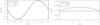Fig. 2 Sheared magnetic field Bz as a functionof x at a midpoint in y (left) and as a function of y for x = −0.15 (right) for β0 of 4/30 at t = 50. The footpoint displacement is D∕L ≈ 0.29. The solid black curve is for the Lare2D results, triple-dot-dashed blue for the relaxation method, dot-dashed red for the 1D approximation, and dashed green for the linearised MHD results.

Fig. 3 Bz against x at the mid-line y = 0 for each method. The time t = 200 and the footpoint displacement is D ≈ 3.9. Left: β0 of 4/3. Right: β0 of 4/300.

3.2 Comparison of B_y

Initially, B_y is the only magnetic field component. Figure 4 shows B_y as a function of x at the mid-line at y = 0 for D∕L ≈ 0.63 (t = 100) in the top row and D∕L ≈ 1.3 (t = 200) in the bottom row corresponding to high β₀ in the left column and low β₀ in the right column. The other parameters are the same as above.

For the Lare2D results with low D∕L ≈ 0.63 the maximum value of B_y is higher than the initial value by about 5% for high β₀, and 10% for low β₀ where non-linear effects are becoming important. Hence, for footpoint displacements smaller than the loop length the variations in B_y are not too significant. For the case of high D∕L ≈ 1.3 the maximum ofB_y is about 20% higher for high β₀ and 30% for low β₀. It can be concluded that for high values of D any assumption that the horizontal variations in the background field are small is not valid.

For the high plasma β₀ case, (left column), only the relaxation results are significantly different from the others for both low and high D∕L, as expected, since this method assumes the field is force-free. Similarly to B_z, in the low β₀ regime in the right column, the relaxation method agrees with the Lare2D and the 1D approaches regardless of the value of the footpoint displacement, D. Interestingly, the approximation for B_z, the shear component, is consistently better than the B_y component, whereas one may expect the same accuracy for both components.

The Lare2D and 1D approaches agree with each other extremely well for 4∕3000 < β₀ < 4∕3 and for D∕L < 2.6, the highest value tested.

The first- and second-order linearised MHD solutions agree reasonably well with the Lare2D results for low D∕L ≈ 0.63 and high β₀. For low β₀ the linear MHD results show a more noticeable discrepancy for small displacement. For large footpoint displacements, D∕L ≈ 1.3 (t = 200) in the bottom row, the second-order linearised MHD results predict a minimum value of B_y that is too low by about 10% for high β₀, and 25% for low β₀ as the non-linear terms become more important. For RMHD, this component is assumed to remain unchanged during the shearing motion. However, we have shown in the other methods that this is not the case, and variations become significant after a short time.

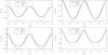Fig. 4 By against x in the midpoint in y for β0 = 4∕3 (left column) and 4/300 (right column) for D ≈ 1.9 at t = 100 (top row) and D ≈ 3.9 at t = 200 (bottom row).

3.3 Comparison of integrated energies

The integrated magnetic energy is shown in Fig. 5 as a function of time for high plasma β₀ (β₀ = 4∕3) and low β₀ (β₀ = 4∕300). The Poynting flux associated with the shearing motion results in the magnetic energy increasing nearly quadratically in time for both values of β₀.

The relaxation approach does not directly give quantities as functions of time. In order to calculate and compare the magnetic energy the magnetic field needs to relax for every value of the displacement. This is limited by resources so the magnetic energy is only calculated for a few values of D, shown as symbols in Fig. 5. These data points agree well with the Lare2D results. As noted for the other quantities, there is a marginal discrepancy for high β₀ which is not present for low β₀. It is interesting to note that the 1D approach correctly matches the results from Lare2D for all times, even when the footpoint displacement is larger than the half-length, L, for example,at t = 400, D∕L ≈ 2.6 using Eq. (67). The analytical estimate from the linearised MHD equations, given in Eq. (58), shows very good agreement up to t = 200, D∕L ≈ 1.3 when the footpoint displacement is about equal to the loop length and is only in error by 10% at t = 400, D∕L ≈ 2.6.

Thus, in comparison to Lare2D, we can conclude that the slow magnetic field evolution is correctly modelled bythe relaxation method and 1D approach for all times, provided the width-to-length ratio, l∕L, is low, and by the linearised MHD method until the footpoint displacement becomes comparable to the loop length, regardless of the size of the plasma β₀. This is notable since once D ~ L one might not have expected the linearisation approach to be valid.

The integrated kinetic energy is shown in Fig. 6 as a function of time for each of the four different values of the initial plasma β₀ given in Table 1. The dashed lines are the kinetic energy estimates given by the first- and second-order linearised MHD method in Eq. (40). There are no estimates from either the relaxation method or the 1D approach, as they are assumed to be in equilibrium. The constant value is only obtained when the Alfvén waves, those excited when the boundary driving velocities are switched on, are dissipated. Because the driving velocities are slow, the integrated kinetic energy is five orders of magnitude lower than the magnetic energy.

What is surprising, at first sight, is that the Lare2D results only really match the prediction from Eq. (40) for an initial high β₀ plasma. As β₀ is reduced, the departure from the constant kinetic energy is much more significant. The reason for this departure is due to the flow along the initial magnetic field direction, v_y (as shown analytically by the linearised MHD method in Sect. 2.5), which is a consequence of the magnetic pressure gradient in y due to the y variation in B_z (see Eq. (38)). The size of the constantflow, G(y), in the second-order solution, is proportional to ${(l_{\text{d}}/l)}^2{(V_0/c_{\text{s}})}^2$, where the diffusion lengthscale, l_d, is defined above and $c_{\text{s}}^2=\gamma p_0/{\rho }_0$ is proportional to the initial gas pressure. The viscosity may be either real or due to numerical dissipation. In both cases, the viscosity damps out both the fast and Alfvén waves generated when the driving is switched on. Once these waves are damped, the plasma can pass through sequences of equilibria. Although ν is low, l_d will eventually become large, which means that p₀ cannot be too low or else this change in density will occur sooner. This steady flow is due to the magnetic pressure gradients introduced by viscosity in the shearing component of the magnetic field, B_1z. Although the magnitude of this flow is small, it is constant in time and it will eventually modify the plasma density (see Sect. 3.4 and the second-order Eq. (48)). In turn, the change in the density will influence the integrated kinetic energy.

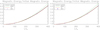Fig. 5 Integrated magnetic energy as a function of time, t. β0: left 4/3, right 4/300.

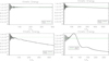Fig. 6 Integrated kinetic energy as a function of time, t. β0: top left 4/3, top right 4/30, bottom left 4/300, and bottom right 4/3000.

3.4 Comparison with ρ

The comparison of the plasma density between the Lare2D results, the linearised MHD method, and the 1D approach is shown in Fig. 7at the midpoint in y for high plasma β₀ (left column), low β₀ (right column) and footpoint displacement of D∕L ≈ 0.63 (top row) and D∕L ≈ 1.3 (bottom row). The relaxation and RMHD methods are not considered as they do not account for variations in density. For high β₀ and low D∕L the agreement among the three methods is very good. The density variations in the x direction are of the order of 4% and all three methods give essentially the same results. However, when the plasma β₀ is low (right column), the density variations are now between 10% and 20% of the initial uniform value, with Lare2D having a general increase in the average value at y = 0. This is due to the variation in y of B_z. These large variations show that non-linear effects are already becoming important.

For highβ₀ and larger footpoint displacement of D∕L ≈ 1.3 (bottom row) the variations are similar to the low β₀ case for low D∕L. This shows that the high β₀ plasma will eventually evolve in the same way, but over a much longer time. Once the footpoint displacement has become large the variations inρ for low β₀ are nearly 60% of the initial uniform value of 1.0, thus are very significant.

The 1D approach agrees with Lare2D for high β₀ for both high and low D∕L. In the case of low β₀ this method predicts the same variation as full MHD, but is displaced slightly because the velocity effects are not included in this approximation.

The first- and second-order linearised MHD results agree reasonably well for small displacement for both high and low β₀. In the case of higher D∕L, non-linear effects become important and the linear results now show a difference with the Lare2D results for both high and low β₀.

The density dependence on the y coordinate was predicted by the second-order solution in Eq. (48). This variation is clearly seen in the results of Lare2D and this is shown as a 2D surface of ρ in Fig. 8, at t = 400 (D∕L ≈ 2.6), for the high β case (left) and the low β₀ case (right).The maximum variation in density increases almost linearly in time, and by t = 400 there is a 15% difference between the maximum and minimum values at x = 0. This y variation is not the same as the rapid boundary layer behaviour seen previously. On the other hand, ρ has almost no y dependence for the high β₀ case (left part of Fig. 8). This clearly illustrates the large variation in density at y = 0 as shown in Fig. 7. This is what causes the kinetic energy to decrease (see Sect. 3.3). The variations in ρ and B_y will modify the Alfvén speed and this can affect the propagation of MHD waves in this plasma.

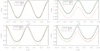Fig. 7 ρ against x at the midpoint in y for β0 of 4/3 (left) and 4/300 (right) for D ≈ 1.9 at time t = 100 (top) and D ≈ 3.9 for t = 200 (bottom).

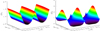Fig. 8 Surfaces of density at t = 400 (D ≈ 7.9) for β0 4/3 (left) and 4/300 (right).

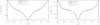Fig. 9 Comparison of jy against x at the midpoint in y for β0 4/3 (left) and 4/300 (right) for D ≈ 3.9 (t = 200).

3.5 Comparison with j_y

The current density is an important quantity to determine accurately in order to calculate force balance and ohmic heating, ηj². The dominant component of the current density is the j_y componentgiven by j_y = −(∂B_z∕∂x). The results of j_y for Lare2D, the 1D approach, and linearisation are shown in Fig. 9 for D∕L ≈ 1.3 for the case of high β₀ (left) and low β₀ (right). The current could be obtained from the relaxation method, but this has not been done here. It is clear that the 1D approach matches the Lare2D results and that the magnitude of the current values exceeds the linear MHD (and the RMHD) estimate by almost a factor of 2 (right part of Fig. 9) for low β₀ values. In general, the magnitude of the current increases as β₀ decreases.

The other component of the current, j_z = (∂B_y∕∂x) is smaller in magnitude than j_y and again both the Lare2D and the 1D approaches agree. RMHD does not predict a value for j_z.

4 Conclusions

A simple footpoint shearing experiment has been investigated to test four different methods against full MHD results of Lare2D Arber et al. (2001) and to contrast the other methods with it. This is the first detailed comparison of the different methods, although Pagano et al. (2013) have compared the relaxation method with an MHD simulation for the onset of a CME, and Dmitruk et al. (2005) have compared RMHD and full MHD in the case of turbulence.

The twomethods that assume that the magnetic field passes through a sequence of equilibria are namely the magneto-frictional relaxation and 1D methods. The relaxation method, in the present form, only studies force-free fields and it provides an excellent match to the Lare2D results for B for low β₀, regardless ofthe footpoint displacement. The inclusion of the gas pressure and plasma density is possible (see Hesse & Birn 1993), but this has not been done here.

The second equilibrium method is the 1D approach, which assumes that the boundary layers at the photospheric footpoints are narrow and so reduces the Grad-Shafranov equation to a simple 1D equation for the flux function. Solutions to the resulting equation give outstanding agreement with the Lare2D results for B_y, B_z, p, ρ, j_y, and j_z for all footpoint displacements and values of β₀. The 1D approach is, of course, derived with this specific experiment in mind. It has been used for the twisting of coronal loops with cylindrical symmetry (see Lothian & Hood 1989; Browning & Hood 1989). The flux function, in this case, is a function of radius alone. Unlike the relaxation method, it is not readily extendable to more complex photospheric footpoint displacements, but it does do exceptionally well for this particular problem.

The simplest dynamical approach is to expand the MHD equations in powers of D∕L, the ratio of the maximum footpoint displacement to the loop half-length. In principal, this should only be valid for D ≪ L. Surprisingly, it has been found that this method provides good agreement for D∕L ≲ 1. One strength of this model is that it can provide useful insight into the system.

Next, we consider Reduced MHD. In general, RMHD is identical to the first-order linear MHD results, and thus is not capable of reproducing the results from Lare2D. This is primarily because its main assumptions do not hold in this situation. While RMHD has the same parallel current component j_y as linear MHD, it does not provide any information about j_z ≈ (∂B_y∕∂x) since there can be no change to B_y. Hence, force balance can only be maintained by balancing the magnetic pressure due to $B_{1z}^2/2$ by the gas pressure instead of through the change to B_y.

There are many possible choices to extend this investigation to more complex systems and to explore the dependencies of this system in more detail. One question is whether this system is dependent on the form of the internal energy equation. The gas pressure and density structures produced by the steady shearing motions result in temperature variations. If thermal conduction is included and the boundary conditions keep the temperature fixed at its initial value, then the temperature will relax towards an isothermal state. The assumption of an isothermal plasma can be included in the 1D method very easily by setting γ = 1. There is still a variation in pressure and density. So the inhomogeneous nature of the resulting plasma is not dependent on the exact form of the internal energy equation.

Further work on the validity of RMHD is required. For this experiment, we can neglect the variations parallel to the initial field whenever the horizontal lengthscales are much shorter than the parallel ones. However, whether RMHD can be used or not depends on the final footpoint location, the total displacement, and how the field lines got there. On the one hand, a simple shear followed by the opposite shear brings the footpoints back to their initial locations, but the field will remain potential. On the other hand, a complete rotation also brings the footpoints to their initial locations, but this time the field is not potential. What is important is how the field gets to the final location and the total Poynting flux that is injected into the corona.

The main message to be taken from this work is that care should be taken not to simply implement a method without first establishing whether the assumptions are valid. The four approximate methods have been used here for a particularly simple shearing experiment. For example, the simple 1D method is inappropriate for more complex and realistic photospheric footpoint motions. However, the magneto-frictional, relaxation method is still applicable provided the displacement of the footpoints from the previousequilibrium state is small. Hence, a simple rotation of the footpoint through 360 degrees can be achieved by splitting the rotation into smaller angles and relaxing before taking the next small rotation. For small angular motions, the relaxation method will quickly reach the nearby equilibrium state. This is then repeated until the complete revolution is achieved (see Meyer et al. 2011, 2012, 2013, for the application of the relaxation approach to the velocities derived from the magnetic carpet). The linearisation of the MHD equations can always be undertaken, but the derivation of an analytical expression for the linear solution with more complex boundary conditions is not certain. Without an expression for the linear steady state, it will be difficult to determine the modifications to the density and main axial field in response to the non-linear driving by the linear steady state. RMHD can certainly be applied to more complex photospheric motions, but we would expect that the quadratic terms, due to the linear terms, will invalidate some of the main assumptions stated in Oughton et al. (2017). Solving the full MHD equations remains the preferred approach, provided sufficient computing resources are available to generate the long time evolution of the magnetic field.

Acknowledgements

The authors thank the referee for the extremely useful comments. A.W.H. and E.E.G. thank Duncan Mackay for the useful discussions on the magneto-frictional method. A.W.H. acknowledges the financial support of STFC through the Consolidated grant, ST/N000609/1, to the University of St Andrews, and E.E.G. acknowledges the STFC studentship, ST/I505999/1. This work used the DIRAC 1, UKMHD Consortium machine at the University of St Andrews and the DiRAC Data Centric system at Durham University, operated by the Institute for Computational Cosmology on behalf of the STFC DiRAC HPC Facility (www.dirac.ac.uk). This equipment was funded by aBIS National E-infrastructure capital grant ST/K00042X/1, STFC capital grant ST/K00087X/1, DiRAC Operations grant ST/K003267/1, and Durham University. DiRAC is part of the National E-Infrastructure.

Appendix A Second-order solutions

We can solve the second-order Eqs. (32)–(37) for v_2x and v_2y. Then we can determine the other variables. We include the viscous heating and dissipation terms.

Taking the time derivative of Eqs. (32) and (33) and using Eqs. (36) and (37), we have $$\begin{array}{lll}\frac{{\partial }^2{v}_{2x}}{\partial t^2}\hfill & =& -\frac{\partial }{\partial x}(-c_{\text{s}}^2\left(\frac{\partial v_{2x}}{\partial x}+\frac{\partial v_{2y}}{\partial y}\right)\hfill \\ & & +(\gamma -1)\nu \left(\frac{k^2{V}_0^2{y}^2}{L^2}{\cos }^2(kx)+\frac{V_0^2}{L^2}{\sin }^2(kx)\right))\hfill \\ & & -\frac{\partial }{\partial x}\left(\frac{V_{\text{A}}^2}{2}\left(\frac{2V_0^2\tau }{L^2}+\frac{\nu k^2{V}_0^2}{V_{\text{A}}^2}\left(\frac{y^2}{L^2}-1\right)\right){\sin }^2(kx)\right)\hfill \\ & & +V_{\text{A}}^2\left(\frac{{\partial }^2{v}_{2x}}{\partial x^2}+\frac{{\partial }^2{v}_{2x}}{\partial y^2}\right)\hfill \\ & & +\nu \frac{\partial }{\partial t}\left(\frac{4}{3}\frac{{\partial }^2{v}_{2x}}{\partial x^2}+\frac{{\partial }^2{v}_{2x}}{\partial y^2}+\frac{1}{3}\frac{{\partial }^2{v}_{2y}}{\partial x\partial y}\right)\hfill \end{array}$$(A.1)

and $$\begin{array}{lll}\frac{{\partial }^2{v}_{2y}}{\partial t^2}\hfill & =& -\frac{\partial }{\partial y}(-c_{\text{s}}^2\left(\frac{\partial v_{2x}}{\partial x}+\frac{\partial v_{2y}}{\partial y}\right)\\ & & +(\gamma -1)\nu \left(\frac{k^2{V}_0^2{y}^2}{L^2}{\cos }^2(kx)+\frac{V_0^2}{L^2}{\sin }^2(kx)\right))\hfill \\ & & -\frac{\partial }{\partial y}\left(\frac{V_{\text{A}}^2}{2}\left(\frac{2V_0^2\tau }{L^2}+\frac{\nu k^2{V}_0^2}{V_{\text{A}}^2}\left(\frac{y^2}{L^2}-1\right)\right){\sin }^2(kx)\right)\\ & & +\nu \frac{\partial }{\partial t}\left(\frac{{\partial }^2{v}_{2y}}{\partial x^2}+\frac{4}{3}\frac{{\partial }^2{v}_{2y}}{\partial y^2}+\frac{1}{3}\frac{{\partial }^2{v}_{2x}}{\partial y\partial x}\right),\end{array}$$(A.2)

where τ = t − t₁. These two equations can be solved by taking $$\begin{array}{l}{v}_{2x}(x,y,t)=(B(y)\tau +C(y))\sin (2kx),\hfill \\ v_{2y}(x,y,t)=(F(y)\tau +E(y))\cos (2kx)+G(y),\hfill \\ B(y)=\frac{\delta }{4k}\left(\frac{\cosh (2ky)}{\cosh (2kL)}-1\right),\hfill \\ G(y)=\nu \frac{(2\gamma -1)k^2{L}^2}{12c_{\text{s}}^2}\left(\frac{V_0^2}{L^2}\right)y\left(1-\frac{y^2}{L^2}\right),\hfill \\ C(y)=\frac{\nu }{2k{V}_{\text{A}}^2}\left(\alpha +\frac{\delta }{2}\right)\left(\frac{\cosh (2ky)}{\cosh (2kL)}\left(2k^2{L}^2+1\right)-\left(2k^2{y}^2+1\right)\right)\hfill \\ +\frac{\nu }{4k{V}_{\text{A}}^2}\left(2c_{\text{s}}^2\kappa -\delta +\frac{2}{3}\alpha \right)\left(\frac{\cosh (2ky)}{\cosh (2kL)}-1\right),\hfill \\ F(y)=\frac{\delta }{4k}\left(\tanh (2kL)\frac{y}{L}-\frac{\sinh (2ky)}{\cosh (2kL)}\right),\hfill \\ E(y)=\frac{2\nu k^2}{3}\left(\left(\alpha +\frac{\delta }{2}\right)\left(\frac{1}{V_{\text{A}}^2}+\frac{1}{c_{\text{s}}^2}\right)+\frac{V_0^2\left(\gamma -\frac{3}{2}\right)}{4L^2{c}_{\text{s}}^2}\right)y^3\hfill \\ +\nu \left(\frac{k^2{V}_0^2}{4c_{\text{s}}^2}+\left(\frac{4\alpha }{3V_{\text{A}}^2}-\frac{V_0^2(\gamma -1)}{2L^2{c}_{\text{s}}^2}\right)+\kappa \left(\frac{c_{\text{s}}^2}{V_{\text{A}}^2}+1\right)\right)y\hfill \\ -\nu \left(L^2\left(\alpha +\frac{\delta }{2}\right)k^2+\frac{c_{\text{s}}^2\kappa }{2}+\frac{2\alpha }{3}\right)\frac{\sinh (2ky)}{V_{\text{A}}^{2}k\cosh (2kL)},\hfill \end{array}$$

where α,  δ, and κ are constants chosen to satisfy the boundary conditions, namely $$\begin{array}{ll}\alpha \hfill & =\frac{\delta }{4kL}\tanh (2kL)-\frac{\delta }{2},\hfill \\ \delta \hfill & =\frac{V_0^2/L^2}{1+(c_{\text{s}}^2/V_{\text{A}}^2)\left(1-\tanh (2kL)/2kL\right)},\hfill \\ \kappa \hfill & =\frac{(V_1+V_2)}{c_{\text{s}}^{2}L\left(kL\left(c_{\text{s}}^2+V_{\text{A}}^2\right)-\frac{1}{2}{c}_{\text{s}}^2\tanh (2kL)\right)},\hfill \end{array}$$

and $$\begin{array}{llll}{V}_1\hfill & =c_{\text{s}}^{2}L\left(k^2\left(\alpha +\frac{\delta }{2}\right)L^2+\frac{2}{3}\alpha \right)\tanh (2kL),V_2\hfill & =-\frac{2}{3}k(\left(c_{\text{s}}^2+V_{\text{A}}^2\right)\left(\alpha +\frac{\delta }{2}\right)k^2{L}^4+\left(\frac{V_0^2\gamma V_{\text{A}}^2{k}^2}{4}+2\alpha c_{\text{s}}^2\right)L^2\hfill & -\frac{3V_0^2{V}_{\text{A}}^2(\gamma -1)}{4})\cdot \hfill \end{array}$$

From the expressions for v_2x and v_2y, we can calculate the other variables as $$\begin{array}{lllllll}\hfill & B_{2x}(x,y,t)=B_0\left(B^{\prime }(y)\frac{{\tau }^2}{2}+C^{\prime }(y)\tau \right)\sin (2kx),\hfill & B_{2y}(x,y,t)=-2k{B}_0\left(B(y)\frac{{\tau }^2}{2}+C(y)\tau )\right)\cos (2kx),\hfill & \frac{{\rho }_2(x,y,t)}{{\rho }_0}=-G^{\prime }(y)\tau +(\left[2kB(y)+F^{\prime }(y)\right]\frac{{\tau }^2}{2}\hfill & +(2kC(y)+E^{\prime }(y))\tau )\cos (2kx),\hfill & p_2(x,y,t)=\frac{\gamma p_0}{{\rho }_0}{\rho }_2\text{nnnotag}\hfill & +(\gamma -1){\rho }_0\nu \tau \left(k^2{V}_{1z}^2{\cos }^{2}kx+{\left(\frac{\partial V_{1z}}{\partial y}\right)}^2{\sin }^{2}kx\right).\hfill \end{array}$$

We note that B_2y and B_2x also have boundary layers and that $$B_{2x}\approx 0,B_{2y}\approx B_0\left(\frac{\delta {\tau }^2}{4}+\frac{\nu c_{\text{s}}^2\kappa \tau }{V_{\text{A}}^2}\right)2\left(\frac{1}{2}-{\sin }^2(kx)\right)$$(A.19)

References

- Arber, T., Longbottom, A., Gerrard, C., & Milne, A. 2001, J. Comput. Phys., 171, 151 [NASA ADS] [CrossRef] [Google Scholar]
- Bowness, R., Hood, A. W., & Parnell, C. E. 2013, A&A, 560, A89 [NASA ADS] [CrossRef] [EDP Sciences] [Google Scholar]
- Browning, P. K., & Hood, A. W. 1989, Sol. Phys., 124, 271 [NASA ADS] [CrossRef] [Google Scholar]
- Dmitruk, P., Matthaeus, W. H., & Oughton, S. 2005, Physics of Plasmas, 12, 112304 [NASA ADS] [CrossRef] [Google Scholar]
- Hesse, M., & Birn, J. 1993, Geophys. Res. Lett., 20, 1451 [NASA ADS] [CrossRef] [Google Scholar]
- Kadomtsev, B. B., & Pogutse, O. P. 1974, JETP, 38, 283 [NASA ADS] [Google Scholar]
- Klimchuk, J. A., & Sturrock, P. A. 1992, ApJ, 385, 344 [NASA ADS] [CrossRef] [Google Scholar]
- Lothian, R. M., & Hood, A. W. 1989, Sol. Phys., 122, 227 [NASA ADS] [CrossRef] [Google Scholar]
- Mackay, D. H., & van Ballegooijen A. A. 2006a, ApJ, 641, 577 [NASA ADS] [CrossRef] [Google Scholar]
- Mackay, D. H., & van Ballegooijen A. A. 2006b, ApJ, 642, 1193 [NASA ADS] [CrossRef] [Google Scholar]
- Mellor, C., Gerrard, C. L., Galsgaard, K., Hood, A. W., & Priest, E. R. 2005, Sol. Phys., 227, 39 [NASA ADS] [CrossRef] [Google Scholar]
- Meyer, K. A., Mackay, D. H., van Ballegooijen, A. A., & Parnell, C. E. 2011, Sol. Phys., 272, 29 [NASA ADS] [CrossRef] [Google Scholar]
- Meyer, K. A., Mackay, D. H., & van Ballegooijen A. A. 2012, Sol. Phys., 278, 149 [NASA ADS] [CrossRef] [Google Scholar]
- Meyer, K. A., Mackay, D. H., van Ballegooijen, A. A., & Parnell, C. E. 2013, Sol. Phys., 286, 357 [NASA ADS] [CrossRef] [Google Scholar]
- Murawski, K., & Goossens, M. 1994, A&A, 286, 952 [NASA ADS] [Google Scholar]
- Oughton, S., Matthaeus, W. H., & Dmitruk, P. 2017, ApJ, 839 [Google Scholar]
- Pagano, P., Mackay, D. H., & Poedts, S. 2013, A&A, 554, A77 [NASA ADS] [CrossRef] [EDP Sciences] [Google Scholar]
- Rappazzo, A. F., Velli, M., & Einaudi, G. 2010, ApJ, 722, 65 [NASA ADS] [CrossRef] [Google Scholar]
- Rappazzo, A. F., Velli, M., & Einaudi, G. 2013, ApJ, 771, 76 [NASA ADS] [CrossRef] [Google Scholar]
- Rosner, R., & Knobloch, E. 1982, ApJ, 262, 349 [NASA ADS] [CrossRef] [Google Scholar]
- Scheper, R. A., & Hassam, A. B. 1999, ApJ, 511, 976 [NASA ADS] [CrossRef] [Google Scholar]
- Schrijver, C. J., De Rosa, M. L., Metcalf, T. R., et al. 2006, Sol. Phys., 235, 161 [Google Scholar]
- Strauss, H. R. 1976, The Physics of Fluids, 19, 134 [NASA ADS] [CrossRef] [Google Scholar]
- Yang, W.-H. 1989, ApJ, 344, 966 [NASA ADS] [CrossRef] [Google Scholar]
- Yang, W.-H. 1990, ApJ, 348, L73 [NASA ADS] [CrossRef] [Google Scholar]
- Yang, W.-H. 1992, ApJ, 392, 465 [NASA ADS] [CrossRef] [Google Scholar]
- Yang, W. H., Sturrock, P. A., & Antiochos, S. K. 1986, ApJ, 309, 383 [NASA ADS] [CrossRef] [Google Scholar]
- Zank, G. P., & Matthaeus, W. H. 1992, J. Plasma Phys., 48, 85 [NASA ADS] [CrossRef] [Google Scholar]