© ESO, 2017

1. Introduction

One of the key questions related to magnetic structures in space plasmas is their stability, that is the analysis of the evolution of perturbations over time. Instabilities are ubiquitous in space plasmas as they can provide the dissipation and transport of momentum over large scales.

The magnetic Rayleigh-Taylor (MRT) instability operates in a variety of astrophysical systems. For example, it manifests itself in buoyant magnetised bubbles identified in clusters of galaxies (Robinson et al. 2004; Jones & De Young 2005; O’Neil et al. 2009), in shells of young supernova remnants (Jun et al. 1995; Jun & Norman 1996), and at the interface between an expanding pulsar wind nebula and its surrounding supernova remnant (Bucciantini et al. 2004).

The MRT instability is also very important in applications to solar physics. Isobe et al. (2005, 2006) proposed that the MRT instability is a possible cause of the filamentary structure in mass and current density in the emerging flux regions. Ryutova et al. (2010) suggested that several dynamic processes taking place in prominences are most probably related to the MRT instabilities. Hilier et al. (2011, 2012a,b) have performed three-dimensional magnetohydrodynamic simulations to investigate the non-linear evolution of the Kippenhahn-Shlüter prominence model due to the MRT instability.

The MRT instability may also affect magnetic threads in solar prominences. The threads are parts of magnetic tubes filled with the colder plasma and with a high density contrast with respect to the coronal plasma. They are quite thin, of the order of 100 km, aligned with the magnetic field and, in many cases, they seem to lie horizontally with respect to the photosphere. Because of their low temperature the thread plasma is only partially ionised. The MRT instability in partially ionised plasmas has been studied both analytically (Díaz et al. 2014) and numerically (Khomenko et al. 2014) under an assumption that the magnetic field both in the dense prominence thread and in the surrounding hot plasma has the same direction. However, observations show (Leroy et al. 1984; Bommier et al. 1994) that the angle between the magnetic field vector and the prominence long axis can be as large as 53° ± 15°. In addition, the magnetic field in the corona can also be tilted with respect to the longitudinal axis of the prominence. This is why in a realistic model the magnetic field at the interface between the prominence and corona has a shear, perfectly justifying our present analysis.

Observations show that the threads have short lifetimes, typically of the order of only 10 min. These observations inspired Terradas et al. (2012) to propose that the magnetic Rayleigh-Taylor instability could be responsible for this phenomenon. They considered a very simple model. The thread was assumed to be a Cartesian slab permeated by a horizontal magnetic field that has the same direction inside the thread and in the surrounding hot plasma. A drawback of this model is that the instability growth rate is unbounded. Perturbations with an arbitrary wavelength propagating perpendicular to the magnetic field are unstable, and the perturbation increment tends to infinity when the wavelength tends to zero.

Ruderman et al. (2014) improved the model suggested by Terradas et al. (2012) including the magnetic shear. They studied the MRT instability of both a single magnetic interface and a slab. In particular, they found that the maximum increment is inversely proportional to the angle between the magnetic field direction inside the thread and in the external plasma. Assuming that the thread lifetime is equal to the inverse of the maximum increment they managed to estimate the shear angle. Ruderman (2015) studied the effect of flow in a thread on the estimation of the shear angle and found that this effect is minor. Ruderman (2017) investigated the MRT instability in a compressible plasma and found that the effect of compressibility on the estimation of the shear angle is also weak.

Terradas et al. (2012), Ruderman et al. (2014), and Ruderman (2015, 2017) used the approximation of ideal plasmas to study the MRT instability. However, as we have already mentioned, due to its low temperature the prominence plasma is only partially ionised. Díaz et al. (2014) showed that in such a plasma ambipolar diffusion has to be taken into account. In this article we investigate the effect of ambipolar diffusion on the MRT instability with sheared magnetic field. Even in the approximation of ideal plasmas the dispersion equation describing the MRT instability in a compressible plasma is very complex and can only be solved numerically. The account of ambipolar diffusion makes the dispersion equation even more complex. Using the incompressible plasma approximation enormously simplifies the analysis and enables to study the problem analytically. Unfortunately, in this approximation the effect of ambipolar diffusion disappears, hence we need to study the effect of ambipolar diffusion in a compressible plasma.

The paper is organised as follows: in Sect. 2, we formulate the problem and introduce the main equations and boundary conditions. Section 3 is devoted to the derivation of the dispersion equation for perturbations of the interface. Analytical and numerical solutions are found in Sect. 4. Finally, our results are summarised and discussed in Sect. 5.

2. Problem formulation

Our study focuses on the stability of a tangential discontinuity also called a magnetic interface in an inviscid infinitely conducting plasma, where the only non-ideal process that we take into account is ambipolar diffusion. The linearised equations describing the plasma motion in the presence of ambipolar diffusion in the single-fluid approximation have been derived by Díaz et al. (2014) and they can be given as

In the above equations u is the plasma velocity, b the magnetic field perturbation, g the gravity acceleration, B the equilibrium magnetic field, ρ₀ and p₀ the equilibrium density and pressure, ρ and p the density and pressure perturbation, μ₀ magnetic permeability of free space, η_A the coefficient of ambipolar diffusion, and γ the ratio of specific heats. The coefficient of ambipolar diffusion is given by ${\mathit{\eta }}_{\mathrm{A}}\mathrm{=}\frac{{\mathit{m}}_{\mathrm{p}}{\mathit{\xi }}_{\mathrm{n}}{\mathit{c}}_{\mathrm{A}}^{\mathrm{2}}}{\mathrm{4}{\mathit{\sigma }}_{\mathrm{in}}\mathrm{(}\mathrm{1}\mathrm{-}{\mathit{\xi }}_{\mathrm{n}}\mathrm{)}}\sqrt{\frac{\mathit{\pi }\mathrm{(}\mathrm{2}\mathrm{-}{\mathit{\xi }}_{\mathrm{n}}\mathrm{)}}{{\mathit{\rho }}_{\mathrm{0}}{\mathit{p}}_{\mathrm{0}}}}\mathit{,}$(5)where m_p is the proton mass, ξ_n the ionisation degree defined as the ratio of the number density of neutrals and the total number density (neutrals plus ions), σ_in ≈ 5 × 10^-19 m² the collisional cross-section for proton-neutral collisions assuming that the neutrals are the hydrogen atoms, and c_A is the Alfvén speed defined as ${\mathit{c}}_{\mathrm{A}}^{\mathrm{2}}\mathrm{=}\frac{{\mathit{B}}^{\mathrm{2}}}{{\mathit{\mu }}_{\mathrm{0}}{\mathit{\rho }}_{\mathrm{0}}}\mathrm{·}$(6)It should be noted that when Díaz et al. (2014) derived the system of Eqs. (1)–(4), they assumed that all the equilibrium quantities are constant. The validity of this assumption is discussed in detail by, e.g. Ruderman (2017). In what follows we also need the expression for the generalised Ohm’s law, where ambipolar diffusion is taken into account. In the linearised form the Ohm’s law reads ${{E}}^{\mathrm{\prime }}\mathrm{\equiv }{E}\mathrm{+}{u}\mathrm{\times }{B}\mathrm{=}\frac{{\mathit{\eta }}_{\mathrm{A}}}{{\mathit{B}}^{\mathrm{2}}}{B}\mathrm{\times }\mathrm{\left[}\mathrm{\right(}\mathrm{\nabla }\mathrm{\times }{b}\mathrm{)}\mathrm{\times }{B}\mathrm{]}\mathit{,}$(7)where E is the electric field. This equation immediately follows from Eq. (3) if we recall the relation between the time derivative of the magnetic field and the curl of the electrical field.

In our analysis we consider the same equilibrium configuration as in Ruderman et al. (2014) and Ruderman (2017). Our working model consists of two semi-infinite regions separated by the xy-plane in Cartesian coordinates x, y, z with the z-axis in the vertical direction (see Fig. 1). The plasma density and background magnetic fields are constant in the two regions, and are given by ${\mathit{\rho }}_{\mathrm{0}}\mathrm{=}\{\begin{array}{c}\\ {\mathit{\rho }}_{\mathrm{1}}\mathit{,}& \mathit{z}\mathit{<}\mathrm{0}\mathit{,}\\ {\mathit{\rho }}_{\mathrm{2}}\mathit{,}& \mathit{z}\mathit{>}\mathrm{0}\mathit{,}\end{array} {B}\mathrm{=}\{\begin{array}{c}\\ {{B}}_{\mathrm{1}}\mathit{,}& \mathit{z}\mathit{<}\mathrm{0}\mathit{,}\\ {{B}}_{\mathrm{2}}\mathit{,}& \mathit{z}\mathit{>}\mathrm{0.}\end{array}$(8)The background magnetic field in both regions is assumed to be parallel to the xy-plane. The major difference between the equilibrium configuration used here and that used by Díaz et al. (2014) is that here we consider a magnetic shear, while Díaz et al. (2014) assumed that the equilibrium magnetic field is the same at the two sides of the interface. In Fig. 1 the angle α denotes the angle between the direction of the two magnetic fields (i.e. a measure of the magnetic shear), while the angle φ determines the direction of the perturbation wave vector with respect to the direction of the magnetic field in the prominence.

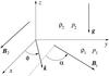Fig. 1 Sketch of the equilibrium. The interface at z = 0 separates the fully ionised solar corona (region 1) and the partially ionised prominence (region 2).

Since we are dealing with a tangential discontinuity, the equilibrium total plasma pressure must be continuous at the interface, so ${\mathit{p}}_{\mathrm{1}}\mathrm{+}\frac{{\mathit{B}}_{\mathrm{1}}^{\mathrm{2}}}{{\mathit{\mu }}_{\mathrm{0}}{\mathit{\rho }}_{\mathrm{1}}}\mathrm{=}{\mathit{p}}_{\mathrm{2}}\mathrm{+}\frac{{\mathit{B}}_{\mathrm{2}}^{\mathrm{2}}}{{\mathit{\mu }}_{\mathrm{0}}{\mathit{\rho }}_{\mathrm{2}}}\mathrm{·}$(9)The equilibrium magnetic field is discontinuous at z = 0. In general, the magnetic field discontinuity cannot exist in a plasma with ambipolar diffusion. However, the only exception is when ambipolar diffusion operates only on one side of the discontinuity. Therefore, in what follows we only consider ambipolar diffusion in the plasma region above the discontinuity, while we assume that the plasma dynamics is described by the ideal MHD equations in the region below the discontinuity. This set-up is a very viable assumption because the plasma below the discontinuity is almost fully ionised, meaning that ξ_n ≈ 0. Then it follows from Eq. (5) that η_A is very small and ambipolar diffusion can be neglected.

Equations (1)–(4) must be supplemented with the boundary conditions at z = 0. Let us define the jump of function f(z) across the interface as $\begin{array}{ccc}\mathrm{\left[}\mathrm{\right[}\mathit{f}\mathrm{\left]}\mathrm{\right]}\mathrm{=}\underset{\mathit{z}\mathrm{\to }\mathrm{+}\mathrm{0}}{\lim }\mathrm{\left[}\mathit{f}\mathrm{\right(}\mathit{z}\mathrm{)}\mathrm{-}\mathit{f}\mathrm{(}\mathrm{-}\mathit{z}\mathrm{\left)}\mathrm{\right]}\mathit{.}& & \end{array}$The first boundary condition is the kinematic boundary condition that expresses the continuity of the normal component of plasma displacement at the interface. In the absence of equilibrium flow this condition reduces in the linear approximation to a very simple form: $\mathrm{\left[}\mathrm{\right[}{\mathit{u}}_{\mathit{z}}\mathrm{\left]}\mathrm{\right]}\mathrm{=}\mathrm{0.}$(10)The second boundary condition is the dynamic boundary condition expressing the continuity of the total pressure. It is written as $\begin{array}{ccc}[[{\mathit{p}}_{\mathrm{0}}\mathrm{+}\mathit{p}\mathrm{+}\frac{\mathrm{(}{B}\mathrm{+}{b}{\mathrm{)}}^{\mathrm{2}}}{\mathrm{2}{\mathit{\mu }}_{\mathrm{0}}}]]\mathrm{=}\mathrm{0} \mathrm{at} \mathit{z}\mathrm{=}\mathit{h}\mathrm{\left(}\mathit{t,x,y}\mathrm{\right)}\mathit{,}& & \end{array}$where z = h(t,x,y) is the equation of the perturbed surface of the discontinuity. We can linearise this equation, and using the Taylor expansion of p₀ near z = 0 and the equation defining the equilibrium pressure (dp₀/ dz = −gρ₀), we eventually obtain $\mathrm{\left[}\mathrm{\right[}\mathit{P}\mathrm{-}\mathit{g}{\mathit{\rho }}_{\mathrm{0}}\mathit{h}\mathrm{\left]}\mathrm{\right]}\mathrm{=}\mathrm{0} \mathrm{at} \mathit{z}\mathrm{=}\mathrm{0}\mathit{,}$(11)where $\mathit{P}\mathrm{=}\mathit{p}\mathrm{+}\frac{{b}\mathrm{·}{B}}{{\mathit{\mu }}_{\mathrm{0}}}$(12)is the perturbation of the total pressure (kinetic plus magnetic). Differentiating this equation with respect to time and using the equation u_z = ∂h/∂t valid in the linear approximation at z = 0 to eliminate h, we finally arrive at $[[\mathit{g}{\mathit{\rho }}_{\mathrm{0}}{\mathit{u}}_{\mathit{z}}\mathrm{-}\frac{\mathit{\partial P}}{\mathit{\partial t}}]]\mathrm{=}\mathrm{0.}$(13)The continuity of the normal component of the plasma velocity and the total pressure perturbation are the only two boundary conditions that must be imposed at a tangential discontinuity in ideal MHD. However, since we consider ambipolar diffusion, we need one more boundary condition that can be obtained using the continuity of tangential component of the electric field calculated in the instantaneous reference frame, where a particular infinitesimal volume of plasma is at rest, i.e. ${{E}}_{\mathit{\tau }}^{\mathrm{\prime }}\mathrm{=}{{E}}^{\mathrm{\prime }}\hspace{0.17em}\mathrm{-}\hspace{0.17em}{{e}}_{\mathit{z}}\mathrm{(}{{e}}_{\mathit{z}}\mathrm{·}{{E}}^{\mathrm{\prime }}\mathrm{)}$ with e_z being the unit vector in the z-direction. Then, using Eq. (7) and taking into account that η_A = 0 for z< 0 we obtain the additional boundary condition that has to be satisfied at z = 0 in the form $\mathrm{(}{\mathit{B}}_{\mathrm{2}}^{\mathrm{2}}{I}\mathrm{-}{{B}}_{\mathrm{2}}{{B}}_{\mathrm{2}}\mathrm{-}{\mathit{B}}_{\mathrm{2}}^{\mathrm{2}}{{e}}_{\mathit{z}}{{e}}_{\mathit{z}}\mathrm{)}\mathrm{·}\mathrm{\nabla }\mathrm{\times }{{b}}_{\mathrm{2}}\mathrm{=}\mathrm{0}\mathit{,}$(14)where I is the unit tensor, e_ze_z denotes the dyadic product of two vectors e_z, and the subscript “2” indicates a quantity defined for z> 0.

3. Derivation of the dispersion equation

In order to derive the dispersion equation for waves propagating along the magnetic interface, we performed a Fourier analysis of the perturbations of all quantities and take them proportional to exp [i(k·r−ωt)], where k = (k_x,k_y,0) and r = (x,y,z). Then, writing u and b as ${u}\mathrm{=}{{u}}_{\mathrm{\perp }}\mathrm{+}{\mathit{u}}_{\mathit{z}}{{e}}_{\mathit{z}}\mathit{,} {b}\mathrm{=}{{b}}_{\mathrm{\perp }}\mathrm{+}{\mathit{b}}_{\mathit{z}}{{e}}_{\mathit{z}}\mathit{,}$(15)we can reduce Eqs. (1)–(4) to

$\begin{array}{ccc}& & \\ & & \\ & & \\ & & \mathit{\omega }{{b}}_{\mathrm{\perp }}\mathrm{=}{B}\mathrm{(}{k}\mathrm{·}{u}\mathrm{)}\mathrm{-}{{u}}_{\mathrm{\perp }}\mathrm{(}{k}\mathrm{·}{B}\mathrm{)}\mathrm{-}\mathrm{i}{B}\frac{\mathrm{d}{\mathit{u}}_{\mathit{z}}}{\mathrm{d}\mathit{z}}\mathrm{-}\frac{\mathrm{i}{\mathit{\eta }}_{\mathrm{A}}}{{\mathit{B}}^{\mathrm{2}}}\{\mathrm{(}{k}\mathrm{·}{B}{\mathrm{)}}^{\mathrm{2}}{{b}}_{\mathrm{\perp }}\\ & & \\ & & \\ & & \end{array}$where c_s is the sound speed defined by ${\mathit{c}}_{\mathrm{s}}^{\mathrm{2}}\mathrm{=}\frac{\mathit{\gamma }{\mathit{p}}_{\mathrm{0}}}{{\mathit{\rho }}_{\mathrm{0}}}\mathrm{·}$(22)When deriving Eqs. (19) and (20) we have used the equation ∇·b = 0.

The boundary condition (13) reduces to $\mathrm{\left[}\mathrm{\right[}\mathit{g}{\mathit{\rho }}_{\mathrm{0}}{\mathit{u}}_{\mathit{z}}\mathrm{+}\mathrm{i}\mathit{\omega P}\mathrm{\left]}\mathrm{\right]}\mathrm{=}\mathrm{0} \mathrm{at}\mathit{z}\mathrm{=}\mathrm{0.}$(23)The boundary condition (14) can be transformed into $\begin{array}{ccc}{k}\mathrm{\times }{{b}}_{\mathrm{\perp }\mathrm{2}}& \mathrm{+}& \mathrm{(}{k}\mathrm{\times }{{e}}_{\mathit{z}}\mathrm{)}{\mathit{b}}_{\mathit{z}\mathrm{2}}\mathrm{-}\mathrm{i}{{e}}_{\mathit{z}}\mathrm{\times }\frac{\mathrm{d}{{b}}_{\mathrm{\perp }\mathrm{2}}}{\mathrm{d}\mathit{z}}\mathrm{-}{{e}}_{\mathit{z}}\mathrm{[}{{e}}_{\mathit{z}}\mathrm{·}\mathrm{(}{k}\mathrm{\times }{{b}}_{\mathrm{\perp }\mathrm{2}}\mathrm{\left)}\mathrm{\right]}\\ & \mathrm{-}& \end{array}$(24)It is straightforward to verify that the projections of the left-hand side of this equation on vectors e_z and B₂ are equal to zero. Hence, the only non-trivial projection is on vector e_z × B₂ and it becomes ${{B}}_{\mathrm{2}}\mathrm{·}\left(\frac{\mathrm{d}{{b}}_{\mathrm{2}}}{\mathrm{d}\mathit{z}}\mathrm{-}\mathrm{i}{k}{\mathit{b}}_{\mathit{z}\mathrm{2}}\right)\mathrm{=}\mathrm{0} \mathrm{at} \mathit{z}\mathrm{=}\mathrm{0.}$(25)Eliminating ρ, u_⊥, and b_⊥ from Eqs. (16)–(21) we obtain the system of equations for u_z, b_z, and P,

$\begin{array}{ccc}& & \\ & & \\ & & [{\mathit{\omega }}^{\mathrm{2}}({\mathit{c}}_{\mathrm{A}}^{\mathrm{2}}\mathrm{+}{\mathit{c}}_{\mathrm{s}}^{\mathrm{2}})\mathrm{-}{\mathit{\omega }}_{\mathrm{A}}^{\mathrm{2}}{\mathit{c}}_{\mathrm{s}}^{\mathrm{2}}\mathrm{-}\mathrm{i}\mathit{\omega }{\mathit{c}}_{\mathrm{s}}^{\mathrm{2}}{\mathit{\eta }}_{\mathrm{A}}(\frac{{\mathrm{d}}^{\mathrm{2}}}{\mathrm{d}{\mathit{z}}^{\mathrm{2}}}\mathrm{-}{\mathit{k}}^{\mathrm{2}})]\mathrm{\Psi }\mathrm{=}\\ & & \end{array}$where $\mathrm{\Psi }\mathrm{=}{\mathit{c}}_{\mathrm{s}}^{\mathrm{2}}\left(\frac{\mathrm{d}{\mathit{u}}_{\mathit{z}}}{\mathrm{d}\mathit{z}}\mathrm{+}\frac{{k}\mathrm{·}{B}}{{\mathit{\mu }}_{\mathrm{0}}{\mathit{\rho }}_{\mathrm{0}}\mathit{\omega }}\frac{\mathrm{d}{\mathit{b}}_{\mathit{z}}}{\mathrm{d}\mathit{z}}\right)\mathrm{-}\frac{\mathrm{i}({\mathit{\omega }}^{\mathrm{2}}\mathrm{-}{\mathit{c}}_{\mathrm{s}}^{\mathrm{2}}{\mathit{k}}^{\mathrm{2}})}{{\mathit{\rho }}_{\mathrm{0}}\mathit{\omega }}\mathit{P,}$(29)and ω_A is the Alfvén frequency defined by ${\mathit{\omega }}_{\mathrm{A}}\mathrm{=}\frac{{k}\mathrm{·}{B}}{\sqrt{{\mathit{\mu }}_{\mathrm{0}}{\mathit{\rho }}_{\mathrm{0}}}}\mathrm{·}$(30)The boundary condition given by Eq. (25) reduces to $\frac{\mathrm{d}{\mathrm{\Psi }}_{\mathrm{2}}}{\mathrm{d}\mathit{z}}\mathrm{-}\frac{\mathit{\omega }\mathrm{(}{k}\mathrm{·}{{B}}_{\mathrm{2}}\mathrm{)}}{{\mathit{\mu }}_{\mathrm{0}}{\mathit{\rho }}_{\mathrm{02}}}{\mathit{b}}_{\mathit{z}\mathrm{2}}\mathrm{=}\mathrm{0.}$(31)Finally, we require that perturbations should be evanescent in the transversal direction; therefore, we impose the condition that all perturbations tend to zero as | z | → ∞.

Eliminating all variables in favour of P in the system of Eqs. (26)–(29) we can obtain the differential equation for P, $\begin{array}{ccc}[{\mathit{\omega }}^{\mathrm{2}}({\mathit{c}}_{\mathrm{A}}^{\mathrm{2}}\mathrm{+}{\mathit{c}}_{\mathrm{s}}^{\mathrm{2}})\mathrm{-}{\mathit{\omega }}_{\mathrm{A}}^{\mathrm{2}}{\mathit{c}}_{\mathrm{s}}^{\mathrm{2}}& \mathrm{-}& \mathrm{i}\mathit{\omega }{\mathit{c}}_{\mathrm{s}}^{\mathrm{2}}{\mathit{\eta }}_{\mathrm{A}}\left(\frac{{\mathrm{d}}^{\mathrm{2}}}{\mathrm{d}{\mathit{z}}^{\mathrm{2}}}\mathrm{-}{\mathit{k}}^{\mathrm{2}}\right)]({\mathit{c}}_{\mathrm{s}}^{\mathrm{2}}\frac{{\mathrm{d}}^{\mathrm{2}}\mathit{P}}{\mathrm{d}{\mathit{z}}^{\mathrm{2}}}\mathrm{+}\mathit{g}\frac{\mathrm{d}\mathit{P}}{\mathrm{d}\mathit{z}}\\ \mathrm{+}({\mathit{\omega }}^{\mathrm{2}}\mathrm{-}{\mathit{k}}^{\mathrm{2}}{\mathit{c}}_{\mathrm{s}}^{\mathrm{2}})\mathit{P})& \mathrm{=}& \end{array}$(32)In order to be able to derive a dispersion relation, we would also need the equations that relate the variables u_z, b_z, and Ψ with P, and they are $\begin{array}{ccc}\mathit{g}\frac{\mathrm{d}{\mathit{u}}_{\mathit{z}}}{\mathrm{d}\mathit{z}}& \mathrm{+}& {\mathit{\omega }}^{\mathrm{2}}{\mathit{u}}_{\mathit{z}}\mathrm{=}\frac{-1}{{\mathit{\rho }}_{\mathrm{0}}[{\mathit{c}}_{\mathrm{A}}^{\mathrm{2}}({\mathit{\omega }}^{\mathrm{2}}\mathrm{-}{\mathit{\omega }}_{\mathrm{A}}^{\mathrm{2}})\mathrm{+}\mathrm{i}\mathit{\omega }{\mathit{\omega }}_{\mathrm{A}}^{\mathrm{2}}{\mathit{\eta }}_{\mathrm{A}}]}\\ & \mathrm{\times }& [{\mathit{\omega }}_{\mathrm{A}}^{\mathrm{2}}{\mathit{\eta }}_{\mathrm{A}}\left({\mathit{c}}_{\mathrm{s}}^{\mathrm{2}}\frac{{\mathrm{d}}^{\mathrm{3}}\mathit{P}}{\mathrm{d}{\mathit{z}}^{\mathrm{3}}}\mathrm{+}\mathit{g}\frac{{\mathrm{d}}^{\mathrm{2}}\mathit{P}}{\mathrm{d}{\mathit{z}}^{\mathrm{2}}}\right)\mathrm{+}\mathrm{(}\mathrm{i}{\mathit{c}}_{\mathrm{A}}^{\mathrm{2}}{\mathit{\omega }}^{\mathrm{3}}\\ & \mathrm{-}& \\ \mathit{g}\frac{\mathrm{d}{\mathit{b}}_{\mathit{z}}}{\mathrm{d}\mathit{z}}& \mathrm{+}& {\mathit{\omega }}^{\mathrm{2}}{\mathit{b}}_{\mathit{z}}\mathrm{=}\frac{\mathit{\omega }\mathrm{(}{k}\mathrm{·}{B}\mathrm{)}}{{\mathit{\rho }}_{\mathrm{0}}[{\mathit{c}}_{\mathrm{A}}^{\mathrm{2}}({\mathit{\omega }}^{\mathrm{2}}\mathrm{-}{\mathit{\omega }}_{\mathrm{A}}^{\mathrm{2}})\mathrm{+}\mathrm{i}\mathit{\omega }{\mathit{\omega }}_{\mathrm{A}}^{\mathrm{2}}{\mathit{\eta }}_{\mathrm{A}}]}({\mathit{c}}_{\mathrm{s}}^{\mathrm{2}}{\mathit{\eta }}_{\mathrm{A}}\frac{{\mathrm{d}}^{\mathrm{3}}\mathit{P}}{\mathrm{d}{\mathit{z}}^{\mathrm{3}}}\\ & \mathrm{+}& \\ \mathit{g}\frac{\mathrm{d\Psi }}{\mathrm{d}\mathit{z}}& \mathrm{+}& \end{array}$Assuming that in each region the dependence of the total pressure on z varies as ~ e^λz we can determine the characteristic equation corresponding to Eq. (32) as $\begin{array}{ccc}\mathit{\omega }{\mathit{\eta }}_{\mathrm{A}}{\mathit{c}}_{\mathrm{s}}^{\mathrm{2}}{\mathit{\lambda }}^{\mathrm{4}}& \mathrm{+}& \mathit{\omega g}{\mathit{\eta }}_{\mathrm{A}}{\mathit{\lambda }}^{\mathrm{3}}\mathrm{+}\mathrm{[}\mathrm{i}{\mathit{\omega }}^{\mathrm{2}}({\mathit{c}}_{\mathrm{A}}^{\mathrm{2}}\mathrm{+}{\mathit{c}}_{\mathrm{s}}^{\mathrm{2}})\mathrm{-}\mathrm{i}{\mathit{\omega }}_{\mathrm{A}}^{\mathrm{2}}{{\mathit{c}}_{\mathrm{s}}^{\mathrm{2}}}^{}\\ & \mathrm{+}& \mathit{\omega }{\mathit{\eta }}_{\mathrm{A}}({\mathit{\omega }}^{\mathrm{2}}\mathrm{-}\mathrm{2}{\mathit{k}}^{\mathrm{2}}{\mathit{c}}_{\mathrm{s}}^{\mathrm{2}}{)}^{\mathrm{]}}{\mathit{\lambda }}^{\mathrm{2}}\mathrm{+}\mathit{\omega g\lambda }(\mathrm{i}\mathit{\omega }\mathrm{-}{\mathit{\eta }}_{\mathrm{A}}{\mathit{k}}^{\mathrm{2}})\\ & \mathrm{+}& \mathrm{i}\mathrm{[}{\mathit{\omega }}^{\mathrm{4}}\mathrm{-}{\mathit{\omega }}^{\mathrm{2}}{\mathit{k}}^{\mathrm{2}}({\mathit{c}}_{\mathrm{A}}^{\mathrm{2}}\mathrm{+}{\mathit{c}}_{\mathrm{s}}^{\mathrm{2}})\mathrm{+}{\mathit{k}}^{\mathrm{2}}{\mathit{\omega }}_{\mathrm{A}}^{\mathrm{2}}{{\mathit{c}}_{\mathrm{s}}^{\mathrm{2}}}^{\mathrm{]}}\\ & \mathrm{-}& \end{array}$(36)Obviously the sign of the parameter λ will be chosen in such a way that the evanescence of the perturbation in the transversal direction is insured. In what follows we determine solutions to Eq. (36) in both regions and then match them at the interface.

3.1. Solution in the lower region

In the lower region (z< 0) η_A = 0, therefore, Eq. (36) reduces to $\begin{array}{ccc}\mathrm{[}{\mathit{\omega }}^{\mathrm{2}}({\mathit{c}}_{\mathrm{A}\mathrm{1}}^{\mathrm{2}}\mathrm{+}{\mathit{c}}_{\mathrm{s}\mathrm{1}}^{\mathrm{2}})\mathrm{-}{\mathit{\omega }}_{\mathrm{A}\mathrm{1}}^{\mathrm{2}}{{\mathit{c}}_{\mathrm{s}\mathrm{1}}^{\mathrm{2}}}^{\mathrm{]}}{\mathit{\lambda }}^{\mathrm{2}}& \mathrm{+}& {\mathit{\omega }}^{\mathrm{2}}\mathit{g\lambda }\\ \mathrm{+}{\mathit{\omega }}^{\mathrm{4}}\mathrm{-}{\mathit{\omega }}^{\mathrm{2}}{\mathit{k}}^{\mathrm{2}}({\mathit{c}}_{\mathrm{A}\mathrm{1}}^{\mathrm{2}}& \mathrm{+}& \end{array}$(37)We assume that this quadratic equation has exactly one root with the positive real part. We denote this root as λ₁. Under this assumption it follows from Eqs. (33) and (34) that the solution decaying as z → −∞ is given by $\begin{array}{ccc}{\mathit{P}}_{\mathrm{1}}& \mathrm{=}& {\mathit{A}}_{\mathrm{1}}{\mathrm{e}}^{{\mathit{\lambda }}_{\mathrm{1}}\mathit{z}}\mathit{,} {\mathit{u}}_{\mathit{z}\mathrm{1}}\mathrm{=}\mathrm{-}\frac{\mathrm{i}\mathit{\omega }{\mathit{A}}_{\mathrm{1}}{\mathrm{e}}^{{\mathit{\lambda }}_{\mathrm{1}}\mathit{z}}({\mathit{\omega }}^{\mathrm{2}}{\mathit{\lambda }}_{\mathrm{1}}\mathrm{+}\mathit{g}{\mathit{k}}^{\mathrm{2}})}{{\mathit{\rho }}_{\mathrm{1}}(\mathit{g}{\mathit{\lambda }}_{\mathrm{1}}\mathrm{+}{\mathit{\omega }}^{\mathrm{2}})({\mathit{\omega }}^{\mathrm{2}}\mathrm{-}{\mathit{\omega }}_{\mathrm{A}\mathrm{1}}^{\mathrm{2}})}\mathit{,}\\ {\mathit{b}}_{\mathit{z}\mathrm{1}}& \mathrm{=}& \end{array}$(38)where A₁ is an arbitrary constant.

3.2. Solution in the upper region

In the upper region (z> 0) we take into account the ambipolar diffusion, i.e. η_A ≠ 0. Now we assume that in this case Eq. (36) has exactly two roots with negative real parts. We denote these roots as −λ₂ and −λ₃. The general solution to Eq. (32) tending to zero as z → ∞ is ${\mathit{P}}_{\mathrm{2}}\mathrm{=}{\mathit{A}}_{\mathrm{2}}{\mathrm{e}}^{\mathrm{-}{\mathit{\lambda }}_{\mathrm{2}}\mathit{z}}\mathrm{+}{\mathit{A}}_{\mathrm{3}}{\mathrm{e}}^{\mathrm{-}{\mathit{\lambda }}_{\mathrm{3}}\mathit{z}}\mathit{,}$(39)where A₂ and A₃ are arbitrary constants. Then it follows from Eqs. (33)–(35) that $\begin{array}{ccc}{\mathit{u}}_{\mathit{z}\mathrm{2}}& \mathrm{=}& \frac{\mathrm{1}}{{\mathit{\rho }}_{\mathrm{2}}\mathit{W}}\sum _{\mathit{j}\mathrm{=}\mathrm{2}}^{\mathrm{3}}\frac{{\mathit{A}}_{\mathit{j}}{\mathrm{e}}^{\mathrm{-}{\mathit{\lambda }}_{\mathit{j}}\mathit{z}}}{{\mathit{\omega }}^{\mathrm{2}}\mathrm{-}\mathit{g}{\mathit{\lambda }}_{\mathit{j}}}\mathrm{[}{\mathit{\eta }}_{\mathrm{A}}{\mathit{\omega }}_{\mathrm{A}\mathrm{2}}^{\mathrm{2}}{\mathit{\lambda }}_{\mathit{j}}^{\mathrm{2}}\mathrm{(}{\mathit{c}}_{\mathrm{s}\mathrm{2}}^{\mathrm{2}}{\mathit{\lambda }}_{\mathit{j}}\mathrm{-}{\mathit{g}}^{\mathrm{)}}\mathrm{+}{\mathit{\lambda }}_{\mathit{j}}{\mathrm{(}\mathrm{i}{\mathit{c}}_{\mathrm{A}\mathrm{2}}^{\mathrm{2}}{\mathit{\omega }}^{\mathrm{3}}}^{}\\ & & \\ {\mathit{b}}_{\mathit{z}\mathrm{2}}& \mathrm{=}& \frac{{k}\mathrm{·}{{B}}_{\mathrm{2}}}{{\mathit{\rho }}_{\mathrm{2}}\mathit{W}}\sum _{\mathit{j}\mathrm{=}\mathrm{2}}^{\mathrm{3}}\frac{{\mathit{A}}_{\mathit{j}}{\mathrm{e}}^{\mathrm{-}{\mathit{\lambda }}_{\mathit{j}}\mathit{z}}}{\mathit{g}{\mathit{\lambda }}_{\mathit{j}}\mathrm{-}{\mathit{\omega }}^{\mathrm{2}}}\{{\mathit{\eta }}_{\mathrm{A}}\mathit{\omega }{\mathit{\lambda }}_{\mathit{j}}^{\mathrm{2}}\mathrm{(}{\mathit{c}}_{\mathrm{s}\mathrm{2}}^{\mathrm{2}}{\mathit{\lambda }}_{\mathit{j}}\mathrm{-}{\mathit{g}}^{\mathrm{)}}\\ & & \\ {\mathrm{\Psi }}_{\mathrm{2}}& \mathrm{=}& \end{array}$where $\mathit{W}\mathrm{=}{\mathit{c}}_{\mathrm{A}\mathrm{2}}^{\mathrm{2}}\mathrm{(}{\mathit{\omega }}^{\mathrm{2}}\mathrm{-}{{\mathit{\omega }}_{\mathrm{A}\mathrm{2}}^{\mathrm{2}}}^{\mathrm{)}}\mathrm{+}\mathit{i\omega }{\mathit{\omega }}_{\mathrm{A}\mathrm{2}}^{\mathrm{2}}{\mathit{\eta }}_{\mathrm{A}}\mathit{.}$(43)

3.3. Matching solutions

At this stage it is convenient to introduce the dimensionless variables

$\begin{array}{ccc}& & \mathit{\zeta }\mathrm{=}\frac{{\mathit{\rho }}_{\mathrm{2}}}{{\mathit{\rho }}_{\mathrm{1}}}\mathit{,}\hspace{0.17em}\mathit{\kappa }\mathrm{=}\frac{\mathit{k}{\mathit{c}}_{\mathrm{A}\mathrm{2}}^{\mathrm{2}}}{\mathit{g}}\mathit{,\sigma }\mathrm{=}\mathrm{-}\frac{\mathrm{i}\mathit{\omega }{\mathit{c}}_{\mathrm{A}\mathrm{2}}}{\mathit{g}}\mathit{,\chi }\mathrm{=}\frac{{\mathit{B}}_{\mathrm{1}}^{\mathrm{2}}}{{\mathit{B}}_{\mathrm{2}}^{\mathrm{2}}}\mathit{,\nu }\mathrm{=}\frac{\mathit{g}{\mathit{\eta }}_{\mathrm{A}}}{{\mathit{c}}_{\mathrm{A}\mathrm{2}}^{\mathrm{3}}}\mathit{,}\\ & & \end{array}$(44)It follows from Eq. (9) that due to the continuity of the equilibrium total pressure we can write $\mathit{\chi }\mathrm{=}\frac{\mathrm{2}{\mathit{\beta }}_{\mathrm{2}}\mathrm{+}\mathit{\gamma }}{\mathrm{2}{\mathit{\beta }}_{\mathrm{1}}\mathrm{+}\mathit{\gamma }}\mathrm{·}$(45)In the dimensionless variables Eqs. (36) and (37) reduce to $\begin{array}{ccc}& & \mathit{\nu \sigma }{\mathit{\beta }}_{\mathrm{2}}{\mathrm{\Lambda }}_{\mathit{j}}^{\mathrm{4}}\mathrm{-}\mathit{\nu \sigma }{\mathrm{\Lambda }}_{\mathit{j}}^{\mathrm{3}}\mathrm{-}[{\mathit{\sigma }}^{\mathrm{2}}\mathrm{(}\mathrm{1}\mathrm{+}{\mathit{\beta }}_{\mathrm{2}}\mathrm{)}\mathrm{+}\mathit{\nu \sigma }({\mathit{\sigma }}^{\mathrm{2}}\mathrm{+}\mathrm{2}{\mathit{\kappa }}^{\mathrm{2}}{\mathit{\beta }}_{\mathrm{2}})\\ & & \mathrm{+}{\mathit{\kappa }}^{\mathrm{2}}{\mathit{\beta }}_{\mathrm{2}}{\cos }^{\mathrm{2}}\mathit{\phi }]{\mathrm{\Lambda }}_{\mathit{j}}^{\mathrm{2}}\mathrm{+}\mathit{\sigma }(\mathit{\sigma }\mathrm{+}{\mathit{\kappa }}^{\mathrm{2}}\mathit{\nu }){\mathrm{\Lambda }}_{\mathit{j}}\mathrm{+}{\mathit{\sigma }}^{\mathrm{4}}\mathrm{+}{\mathit{\sigma }}^{\mathrm{2}}{\mathit{\kappa }}^{\mathrm{2}}(\mathrm{1}\mathrm{+}{\mathit{\beta }}_{\mathrm{2}})\\ & & \end{array}$(46)$\begin{array}{ccc}& & \mathit{\chi \zeta }[{\mathit{\sigma }}^{\mathrm{2}}\mathrm{(}\mathrm{1}\mathrm{+}{\mathit{\beta }}_{\mathrm{1}}\mathrm{)}\mathrm{+}{\mathit{\beta }}_{\mathrm{1}}\mathit{\chi \zeta }{\mathit{\kappa }}^{\mathrm{2}}{\cos }^{\mathrm{2}}\mathrm{(}\mathit{\phi }\mathrm{-}\mathit{\alpha }\mathrm{)}]{\mathrm{\Lambda }}_{\mathrm{1}}^{\mathrm{2}}\mathrm{+}{\mathit{\sigma }}^{\mathrm{2}}{\mathrm{\Lambda }}_{\mathrm{1}}\\ & & \end{array}$(47)In Eq. (46) the index j takes the values j = 2,3. In what follows we only consider unstable modes and make an assumption that the value of σ corresponding to these modes is real. Since the value of the dimensionless quantity σ is positive, it immediately follows that Eq. (47) has exactly one real positive root. It is proved in Appendix A that, for σ> 0, Eq. (46) has exactly two real positive roots.

To match the solutions in the lower and upper regions we substitute them in the boundary conditions Eqs. (10), (23), and (25). This yields $\begin{array}{ccc}\frac{\mathit{\zeta \sigma }{\mathit{A}}_{\mathrm{1}}({\mathit{\sigma }}^{\mathrm{2}}{\mathrm{\Lambda }}_{\mathrm{1}}\mathrm{-}{\mathit{\kappa }}^{\mathrm{2}})}{({\mathrm{\Lambda }}_{\mathrm{1}}\mathrm{-}{\mathit{\sigma }}^{\mathrm{2}})[{\mathit{\sigma }}^{\mathrm{2}}\mathrm{+}\mathit{\chi \zeta }{\mathit{\kappa }}^{\mathrm{2}}{\cos }^{\mathrm{2}}\mathrm{(}\mathit{\phi }\mathrm{-}\mathit{\alpha })\mathrm{]}}& \mathrm{-}& \frac{\mathrm{1}}{\begin{array}{c}\mathrm{􏽥}\\ \mathit{W}\end{array}}\sum _{\mathit{j}\mathrm{=}\mathrm{2}}^{\mathrm{3}}\frac{{\mathit{A}}_{\mathit{j}}}{{\mathit{\sigma }}^{\mathrm{2}}\mathrm{+}{\mathrm{\Lambda }}_{\mathit{j}}}\\ \mathrm{\times }\mathrm{[}\mathit{\nu }{\mathrm{\Lambda }}_{\mathit{j}}^{\mathrm{2}}{\mathit{\kappa }}^{\mathrm{2}}\mathrm{(}{\mathit{\beta }}_{\mathrm{2}}{\mathrm{\Lambda }}_{\mathit{j}}\mathrm{-}\mathrm{1}\mathrm{)}{\cos }^{\mathrm{2}}{\mathit{\phi }}^{}\mathrm{+}& {\mathrm{\Lambda }}_{\mathit{j}}& \mathrm{(}{\mathit{\sigma }}^{\mathrm{3}}\mathrm{-}\mathit{\nu }{\mathit{\beta }}_{\mathrm{2}}{\mathit{\kappa }}^{\mathrm{4}}{\cos }^{\mathrm{2}}{\mathit{\phi }}^{\mathrm{)}}\\ \mathrm{+}{\mathit{\kappa }}^{\mathrm{2}}(\mathit{\sigma }& \mathrm{+}& \end{array}$(48)$\begin{array}{ccc}& & \frac{\mathit{\sigma }{\mathit{A}}_{\mathrm{1}}\mathit{U}}{({\mathrm{\Lambda }}_{\mathrm{1}}\mathrm{-}{\mathit{\sigma }}^{\mathrm{2}})[{\mathit{\sigma }}^{\mathrm{2}}\mathrm{+}\mathit{\chi \zeta }{\mathit{\kappa }}^{\mathrm{2}}{\cos }^{\mathrm{2}}\mathrm{(}\mathit{\phi }\mathrm{-}\mathit{\alpha })\mathrm{]}}\\ & & \mathrm{-}\frac{\mathrm{1}}{\begin{array}{c}\mathrm{􏽥}\\ \mathit{W}\end{array}}\sum _{\mathit{j}\mathrm{=}\mathrm{2}}^{\mathrm{3}}\frac{{\mathit{A}}_{\mathit{j}}}{{\mathit{\sigma }}^{\mathrm{2}}\mathrm{+}{\mathrm{\Lambda }}_{\mathit{j}}}\mathrm{\{}\mathit{\nu }{\mathit{\kappa }}^{\mathrm{2}}{\mathrm{\Lambda }}_{\mathit{j}}^{\mathrm{2}}\mathrm{(}{\mathit{\beta }}_{\mathrm{2}}{\mathrm{\Lambda }}_{\mathit{j}}\mathrm{-}\mathrm{1}\mathrm{)}{\cos }^{\mathrm{2}}\mathit{\phi }\\ & & \mathrm{-}{\mathrm{\Lambda }}_{\mathit{j}}{\mathit{\kappa }}^{\mathrm{2}}[\mathit{\sigma }\mathrm{+}\mathit{\nu }({\mathit{\sigma }}^{\mathrm{2}}\mathrm{+}{\mathit{\beta }}_{\mathrm{2}}{\mathit{\kappa }}^{\mathrm{2}})]{\cos }^{\mathrm{2}}\mathit{\phi }\mathrm{-}\mathit{\nu }{\mathit{\kappa }}^{\mathrm{2}}({\mathit{\sigma }}^{\mathrm{4}}\mathrm{-}{\mathit{\kappa }}^{\mathrm{2}}){\cos }^{\mathrm{2}}\mathit{\phi }\\ & & \end{array}$(49)$\sum _{\mathit{j}\mathrm{=}\mathrm{2}}^{\mathrm{3}}\frac{{\mathit{A}}_{\mathit{j}}{\mathit{Q}}_{\mathit{j}}}{{\mathit{\sigma }}^{\mathrm{2}}\mathrm{+}{\mathrm{\Lambda }}_{\mathit{j}}}\mathrm{=}\mathrm{0}\mathit{,}$(50)where we used the notation

$\begin{array}{ccc}& & \\ & & \\ & & {\mathit{Q}}_{\mathit{j}}\mathrm{=}{\mathrm{\Lambda }}_{\mathit{j}}({\mathit{\sigma }}^{\mathrm{2}}\mathrm{+}{\mathit{\kappa }}^{\mathrm{2}}{\cos }^{\mathrm{2}}\mathit{\phi })({\mathit{\beta }}_{\mathrm{2}}{\mathrm{\Lambda }}_{\mathit{j}}^{\mathrm{2}}\mathrm{-}{\mathrm{\Lambda }}_{\mathit{j}}\mathrm{-}{\mathit{\beta }}_{\mathrm{2}}{\mathit{\kappa }}^{\mathrm{2}})\\ & & \end{array}$The constant A₁ can be eliminated using Eqs. (48) and (49) to obtain $\sum _{\mathit{j}\mathrm{=}\mathrm{2}}^{\mathrm{3}}\frac{{\mathit{A}}_{\mathit{j}}{\mathit{S}}_{\mathit{j}}}{{\mathit{\sigma }}^{\mathrm{2}}\mathrm{+}{\mathrm{\Lambda }}_{\mathit{j}}}\mathrm{=}\mathrm{0}\mathit{,}$(54)where $\begin{array}{ccc}{\mathit{S}}_{\mathit{j}}& \mathrm{=}& \mathit{\zeta }({\mathit{\sigma }}^{\mathrm{2}}{\mathrm{\Lambda }}_{\mathrm{1}}\mathrm{-}{\mathit{\kappa }}^{\mathrm{2}})\mathrm{\{}\mathit{\nu }{\mathit{\kappa }}^{\mathrm{2}}{\mathrm{\Lambda }}_{\mathit{j}}^{\mathrm{2}}\mathrm{(}{\mathit{\beta }}_{\mathrm{2}}{\mathrm{\Lambda }}_{\mathit{j}}\mathrm{-}\mathrm{1}\mathrm{)}{\cos }^{\mathrm{2}}{\mathit{\phi }}^{}\\ & & \mathrm{-}{\mathrm{\Lambda }}_{\mathit{j}}{\mathit{\kappa }}^{\mathrm{2}}[\mathit{\sigma }\mathrm{+}\mathit{\nu }({\mathit{\sigma }}^{\mathrm{2}}\mathrm{+}{\mathit{\beta }}_{\mathrm{2}}{\mathit{\kappa }}^{\mathrm{2}})]{\cos }^{\mathrm{2}}\mathit{\phi }\\ & & \mathrm{-}\mathit{\nu }{\mathit{\kappa }}^{\mathrm{2}}({\mathit{\sigma }}^{\mathrm{4}}\mathrm{-}{\mathit{\kappa }}^{\mathrm{2}}){\cos }^{\mathrm{2}}\mathit{\phi }\mathrm{-}\mathit{\sigma }({\mathit{\sigma }}^{\mathrm{4}}\mathrm{+}{\mathit{\sigma }}^{\mathrm{2}}{\mathit{\kappa }}^{\mathrm{2}}{\cos }^{\mathrm{2}}\mathit{\phi }\mathrm{-}{\mathit{\kappa }}^{\mathrm{2}})\}\\ & & \mathrm{-}\mathit{U}\mathrm{[}\mathit{\nu }{\mathrm{\Lambda }}_{\mathit{j}}^{\mathrm{2}}{\mathit{\kappa }}^{\mathrm{2}}\mathrm{(}{\mathit{\beta }}_{\mathrm{2}}{\mathrm{\Lambda }}_{\mathit{j}}\mathrm{-}\mathrm{1}\mathrm{)}{\cos }^{\mathrm{2}}{\mathit{\phi }}^{}\\ & & \end{array}$(55)Equations (50) and (54) constitute the system of two linear homogeneous algebraic equations for A₂ and A₃. The condition of existence of non-trivial solutions to this system gives the dispersion equation ${\mathit{Q}}_{\mathrm{2}}{\mathit{S}}_{\mathrm{3}}\mathrm{-}{\mathit{Q}}_{\mathrm{3}}{\mathit{S}}_{\mathrm{2}}\mathrm{=}\mathrm{0.}$(56)Equations (46), (47), and (56) determine the dependence of σ on the value of κ.

4. Investigation of the dispersion equation

4.1. Analytical results

4.1.1. Critical wavenumber

Ruderman (2017) studied the MRT stability of a magnetic interface in the approximation of ideal MHD. He showed that a normal mode is only unstable when the wavenumber is smaller than the critical wavenumber. This critical wavenumber is independent of the plasma β and is the same as that obtained by Ruderman et al. (2014) in the approximation of incompressible plasma. We will now show that this result remains valid even when the ambipolar diffusion is taken into account, i.e. in partially ionised plasmas.

Since for unstable modes the value of σ was assumed to be real, we obtain that σ → 0 when κ → κ_c, where κ_c is the critical wavenumber in the dimensionless form. When σ → 0 it follows from Eq. (47) that . It is easy to show that in this limit we can obtain from Eq. (46) that ${\mathrm{\Lambda }}_{\mathrm{2}}\mathrm{=}\mathit{\kappa }\mathrm{+}\mathrm{𝒪}\mathrm{\left(}\mathit{\sigma }\mathrm{\right)}\mathit{,} {\mathrm{\Lambda }}_{\mathrm{3}}\mathrm{=}\frac{\mathit{\kappa }\cos \mathit{\phi }}{\sqrt{\mathit{\nu \sigma }}}\mathrm{+}\mathrm{𝒪}\mathrm{\left(}\mathrm{1}\mathrm{\right)}\mathit{.}$(57)Substituting these results into Eqs. (53) and (55) yields $\begin{array}{ccc}{\mathit{Q}}_{\mathrm{2}}& \mathrm{=}& \\ {\mathit{S}}_{\mathrm{2}}& \mathrm{=}& \end{array}$Using these estimations we obtain from Eq. (56) that S₂/σ → 0 as σ → 0. As a result we arrive at ${\mathit{\kappa }}_{\mathrm{c}}\mathrm{=}\frac{\mathit{\zeta }\mathrm{-}\mathrm{1}}{\mathit{\zeta }\mathrm{[}{\cos }^{\mathrm{2}}\mathit{\phi }\mathrm{+}\mathit{\chi }{\cos }^{\mathrm{2}}\mathrm{(}\mathit{\phi }\mathrm{-}\mathit{\alpha }\mathrm{\left)}\mathrm{\right]}}\mathit{,}$(60)which is identical to the expression for κ_c obtained by Ruderman et al. (2014) and Ruderman (2017). A normal mode is unstable when κ<κ_c and stable otherwise. The above equation also means that there are particular values of angles (i.e. α = 0,φ = (2n + 1)π/ 2) for which the critical wavenumber is infinity, i.e. all waves are unstable. This corresponds to the case of parallel magnetic fields at both sides.

4.1.2. Approximation of ideal MHD

Next we show that the dispersion equation Eq. (56) reduces to the dispersion equation derived by Ruderman (2017) in the approximation of ideal MHD, i.e. when ν → 0. Let us introduce the same notation as in Ruderman (2017), in particular $\begin{array}{c}\\ {\mathrm{\Psi }}_{\mathrm{1}}\mathrm{=}{\mathit{\sigma }}^{\mathrm{2}}\mathrm{+}\mathit{\chi \zeta }{\mathit{\kappa }}^{\mathrm{2}}{\cos }^{\mathrm{2}}\mathrm{(}\mathit{\phi }\mathrm{-}\mathit{\alpha }\mathrm{)}\mathit{,}\\ {\mathrm{\Psi }}_{\mathrm{2}}\mathrm{=}{\mathit{\sigma }}^{\mathrm{2}}\mathrm{+}{\mathit{\kappa }}^{\mathrm{2}}{\cos }^{\mathrm{2}}\mathit{\phi ,}\\ {\mathrm{\Phi }}_{\mathrm{1}}\mathrm{=}{\mathit{\sigma }}^{\mathrm{2}}\mathrm{(}{\mathit{\beta }}_{\mathrm{1}}\mathrm{+}\mathrm{1}\mathrm{)}\mathrm{+}{\mathit{\beta }}_{\mathrm{1}}\mathit{\chi \zeta }{\mathit{\kappa }}^{\mathrm{2}}{\cos }^{\mathrm{2}}\mathrm{(}\mathit{\phi }\mathrm{-}\mathit{\alpha }\mathrm{)}\mathit{,}\\ {\mathrm{\Phi }}_{\mathrm{2}}\mathrm{=}{\mathit{\sigma }}^{\mathrm{2}}\mathrm{(}{\mathit{\beta }}_{\mathrm{2}}\mathrm{+}\mathrm{1}\mathrm{)}\mathrm{+}{\mathit{\beta }}_{\mathrm{2}}{\mathit{\kappa }}^{\mathrm{2}}{\cos }^{\mathrm{2}}\mathit{\phi ,}\\ {\mathrm{\Delta }}_{\mathrm{1}}\mathrm{=}{\mathit{\sigma }}^{\mathrm{4}}\mathrm{+}\mathit{\chi \zeta }{\mathit{\kappa }}^{\mathrm{2}}{\mathit{\sigma }}^{\mathrm{2}}\mathrm{(}{\mathit{\beta }}_{\mathrm{1}}\mathrm{+}\mathrm{1}\mathrm{)}\mathrm{+}{\mathit{\beta }}_{\mathrm{1}}{\mathit{\chi }}^{\mathrm{2}}{\mathit{\zeta }}^{\mathrm{2}}{\mathit{\kappa }}^{\mathrm{4}}{\cos }^{\mathrm{2}}\mathrm{(}\mathit{\phi }\mathrm{-}\mathit{\alpha }\mathrm{)}\mathit{,}\\ {\mathrm{\Delta }}_{\mathrm{2}}\mathrm{=}{\mathit{\sigma }}^{\mathrm{4}}\mathrm{+}{\mathit{\kappa }}^{\mathrm{2}}{\mathit{\sigma }}^{\mathrm{2}}\mathrm{(}{\mathit{\beta }}_{\mathrm{2}}\mathrm{+}\mathrm{1}\mathrm{)}\mathrm{+}{\mathit{\beta }}_{\mathrm{2}}{\mathit{\kappa }}^{\mathrm{4}}{\cos }^{\mathrm{2}}\mathit{\phi }\mathit{.}\end{array}$(61)Then we obtain from Eqs. (46), and (47) that $\begin{array}{ccc}{\mathrm{\Lambda }}_{\mathrm{1}}& \mathrm{=}& \\ {\mathrm{\Lambda }}_{\mathrm{2}}& \mathrm{=}& \end{array}$Using Eq. (63) we obtain the estimates , , , and . Then it follows from Eq. (56) in the leading order approximation with respect to ν that S₂ = 0. Taking ν = 0 in this equation we obtain $\begin{array}{ccc}& & \mathit{\zeta }({\mathit{\sigma }}^{\mathrm{2}}{\mathrm{\Lambda }}_{\mathrm{1}}\mathrm{-}{\mathit{\kappa }}^{\mathrm{2}})\mathrm{(}{\mathit{\sigma }}^{\mathrm{2}}{\mathrm{\Psi }}_{\mathrm{2}}\mathrm{+}{\mathit{\kappa }}^{\mathrm{2}}{\mathrm{\Lambda }}_{\mathrm{2}}{\cos }^{\mathrm{2}}\mathit{\phi }\mathrm{-}{\mathit{\kappa }}^{\mathrm{2}}\mathrm{)}\\ & & \end{array}$(64)Multiplying this equation by $\begin{array}{ccc}\left[\mathit{\chi \zeta }{\mathrm{\Psi }}_{\mathrm{1}}({\mathit{\sigma }}^{\mathrm{2}}{\mathrm{\Lambda }}_{\mathrm{1}}\mathrm{+}{\mathit{\kappa }}^{\mathrm{2}})\mathrm{+}{\mathit{\sigma }}^{\mathrm{4}}\right]\left[{\mathrm{\Psi }}_{\mathrm{2}}({\mathit{\sigma }}^{\mathrm{2}}{\mathrm{\Lambda }}_{\mathrm{2}}\mathrm{-}{\mathit{\kappa }}^{\mathrm{2}})\mathrm{-}{\mathit{\sigma }}^{\mathrm{4}}\right]\mathit{,}& & \end{array}$and using the identities $\begin{array}{ccc}({\mathit{\sigma }}^{\mathrm{2}}{\mathrm{\Lambda }}_{\mathrm{1}}\mathrm{-}{\mathit{\kappa }}^{\mathrm{2}})\left[\mathit{\chi \zeta }{\mathrm{\Psi }}_{\mathrm{1}}({\mathit{\sigma }}^{\mathrm{2}}{\mathrm{\Lambda }}_{\mathrm{1}}\mathrm{+}{\mathit{\kappa }}^{\mathrm{2}})\mathrm{+}{\mathit{\sigma }}^{\mathrm{4}}\right]\mathrm{=}{\mathit{\sigma }}^{\mathrm{4}}\mathrm{(}{\mathrm{\Delta }}_{\mathrm{1}}\mathrm{-}{\mathit{\kappa }}^{\mathrm{2}}\mathrm{)}\mathrm{-}\mathit{\chi \zeta }{\mathit{\kappa }}^{\mathrm{4}}{\mathrm{\Psi }}_{\mathrm{1}}\mathit{,}& & \end{array}$$\begin{array}{ccc}({\mathit{\sigma }}^{\mathrm{2}}{\mathrm{\Lambda }}_{\mathrm{2}}\mathrm{+}{\mathit{\kappa }}^{\mathrm{2}})\left[{\mathrm{\Psi }}_{\mathrm{2}}({\mathit{\sigma }}^{\mathrm{2}}{\mathrm{\Lambda }}_{\mathrm{1}}\mathrm{+}{\mathit{\kappa }}^{\mathrm{2}})\mathrm{-}{\mathit{\sigma }}^{\mathrm{4}}\right]\mathrm{=}{\mathit{\sigma }}^{\mathrm{4}}\mathrm{(}{\mathrm{\Delta }}_{\mathrm{2}}\mathrm{-}{\mathit{\kappa }}^{\mathrm{2}}\mathrm{)}\mathrm{-}{\mathit{\kappa }}^{\mathrm{4}}{\mathrm{\Psi }}_{\mathrm{2}}\mathit{,}& & \end{array}$we transform Eq. (64) to

$\begin{array}{ccc}& & \mathit{\zeta }\mathrm{[}{\mathit{\sigma }}^{\mathrm{4}}\mathrm{(}{\mathrm{\Delta }}_{\mathrm{1}}\mathrm{-}{\mathit{\kappa }}^{\mathrm{2}}\mathrm{)}\mathrm{-}\mathit{\chi \zeta }{\mathit{\kappa }}^{\mathrm{4}}{\mathrm{\Psi }}_{\mathrm{1}}\mathrm{]}\mathrm{\{}{\mathit{\sigma }}^{\mathrm{2}}{\mathit{\kappa }}^{\mathrm{2}}{\mathrm{\Phi }}_{\mathrm{2}}{\mathrm{\Lambda }}_{\mathrm{2}}^{\mathrm{2}}{\cos }^{\mathrm{2}}{\mathit{\phi }}^{}\\ & & \mathrm{+}\mathrm{[}{\mathit{\sigma }}^{\mathrm{2}}{\mathrm{\Phi }}_{\mathrm{2}}\mathrm{(}{\mathit{\sigma }}^{\mathrm{2}}{\mathrm{\Psi }}_{\mathrm{2}}\mathrm{-}{\mathit{\kappa }}^{\mathrm{2}}\mathrm{)}\mathrm{-}\mathrm{(}{\mathit{\kappa }}^{\mathrm{2}}{\mathrm{\Phi }}_{\mathrm{2}}\mathrm{+}{\mathit{\sigma }}^{\mathrm{4}}\mathrm{)}{\mathit{\kappa }}^{\mathrm{2}}{\cos }^{\mathrm{2}}{\mathit{\phi }}^{\mathrm{]}}{\mathrm{\Lambda }}_{\mathrm{2}}\\ & & \mathrm{-}\mathrm{(}{\mathit{\sigma }}^{\mathrm{2}}{\mathrm{\Psi }}_{\mathrm{2}}\mathrm{-}{\mathit{\kappa }}^{\mathrm{2}}\mathrm{)}\mathrm{(}{\mathit{\kappa }}^{\mathrm{2}}{\mathrm{\Phi }}_{\mathrm{2}}\mathrm{+}{\mathit{\sigma }}^{\mathrm{4}}\mathrm{)}\}\mathrm{-}\mathrm{[}{\mathit{\sigma }}^{\mathrm{4}}\mathrm{(}{\mathrm{\Delta }}_{\mathrm{2}}\mathrm{-}{\mathit{\kappa }}^{\mathrm{2}}\mathrm{)}\mathrm{-}{\mathit{\kappa }}^{\mathrm{4}}{\mathrm{\Psi }}_{\mathrm{1}}\mathrm{]}\\ & & \mathrm{\times }\hspace{0.17em}\{{\mathit{\chi }}^{\mathrm{2}}{\mathit{\zeta }}^{\mathrm{2}}{\mathit{\sigma }}^{\mathrm{2}}{\mathit{\kappa }}^{\mathrm{2}}{\mathrm{\Phi }}_{\mathrm{1}}{\mathrm{\Lambda }}_{\mathrm{1}}^{\mathrm{2}}{\cos }^{\mathrm{2}}\mathrm{(}\mathit{\phi }\mathrm{-}\mathit{\alpha }\mathrm{)}\mathrm{-}\mathit{\chi \zeta }\mathrm{[}{\mathit{\sigma }}^{\mathrm{2}}{\mathrm{\Phi }}_{\mathrm{1}}{\mathrm{(}{\mathit{\sigma }}^{\mathrm{2}}{\mathrm{\Psi }}_{\mathrm{1}}\mathrm{-}{\mathit{\kappa }}^{\mathrm{2}}\mathrm{)}}^{}\\ & & \mathrm{-}\mathrm{(}\mathit{\chi \zeta }{\mathit{\kappa }}^{\mathrm{2}}{\mathrm{\Phi }}_{\mathrm{2}}\mathrm{+}{\mathit{\sigma }}^{\mathrm{4}}\mathrm{)}{\mathit{\kappa }}^{\mathrm{2}}{\cos }^{\mathrm{2}}\mathrm{(}\mathit{\phi }\mathrm{-}\mathit{\alpha }{\mathrm{)}}^{\mathrm{]}}{\mathrm{\Lambda }}_{\mathrm{1}}\\ & & \end{array}$(65)Now, with the aid of Eqs. (61)–(63), after long but straightforward calculation we reduce Eq. (65) to $\begin{array}{ccc}\mathit{F}\mathrm{\left(}\mathit{\sigma ,}{\mathit{\beta }}_{\mathrm{1}}\mathit{,}{\mathit{\beta }}_{\mathrm{2}}\mathrm{\right)}& \mathrm{\equiv }& \frac{\mathit{\zeta }{\mathrm{\Psi }}_{\mathrm{2}}}{{\mathrm{\Delta }}_{\mathrm{2}}}({\mathit{\sigma }}^{\mathrm{2}}\mathrm{+}\sqrt{{\mathit{\sigma }}^{\mathrm{4}}\mathrm{+}\mathrm{4}{\mathrm{\Delta }}_{\mathrm{2}}{\mathrm{\Phi }}_{\mathrm{2}}})\\ & & \end{array}$(66)This is exactly the dispersion equation obtained by Ruderman (2017) in the approximation of ideal MHD. We verified numerically for a very wide range of parameter variation that, for κ ∈ (0,κ_c), F(σ,β₁,β₂) is a monotonically increasing function of σ when σ> 0. Since F(σ,β₁,β₂) → 2(ζ−1)(κ/κ_c) as σ → 0, and F(σ,β₁,β₂) → ∞ as σ → ∞, we conclude that Eq. (66) has exactly one positive root when κ<κ_c, and no positive roots when κ>κ_c.

4.1.3. Approximation of incompressible plasma

Finally, we consider the approximation of incompressible plasma and take β₁ = β₂ = β → ∞. Then it follows from Eqs. (46) and (47) that $\begin{array}{c}\\ {\mathrm{\Lambda }}_{\mathrm{1}}\mathrm{=}\mathit{\kappa }\mathrm{+}\mathrm{𝒪}({\mathit{\beta }}^{-1})\mathit{,}\\ {\mathrm{\Lambda }}_{\mathrm{2}}\mathrm{=}\mathit{\kappa }\mathrm{+}\frac{{\mathit{\beta }}^{-1}{\mathit{\sigma }}^{\mathrm{2}}({\mathit{\sigma }}^{\mathrm{2}}\mathrm{+}\mathit{\kappa })}{\mathrm{2}\mathit{\kappa }\left({\mathit{\sigma }}^{\mathrm{2}}\mathrm{+}{\mathit{\kappa }}^{\mathrm{2}}{\cos }^{\mathrm{2}}\mathit{\phi }\right)}\mathrm{+}\mathrm{𝒪}({\mathit{\beta }}^{-2})\mathit{,}\\ {\mathrm{\Lambda }}_{\mathrm{3}}\mathrm{=}\sqrt{{\mathit{\kappa }}^{\mathrm{2}}\mathrm{+}\frac{{\mathit{\sigma }}^{\mathrm{2}}\mathrm{+}{\mathit{\kappa }}^{\mathrm{2}}{\cos }^{\mathrm{2}}\mathit{\phi }}{\mathit{\nu \sigma }}}\mathrm{+}\mathrm{𝒪}({\mathit{\beta }}^{-1})\mathit{.}\end{array}$(67)Using these results we obtain the estimates ${\mathit{Q}}_{\mathrm{2}}\mathrm{=}\mathrm{𝒪}({\mathit{\beta }}^{-1})\mathit{,} {\mathit{Q}}_{\mathrm{3}}\mathrm{=}\mathrm{𝒪}\mathrm{\left(}\mathit{\beta }\mathrm{\right)}\mathit{,} {\mathit{S}}_{\mathrm{3}}\mathrm{=}\mathrm{𝒪}\mathrm{\left(}\mathit{\beta }\mathrm{\right)}\mathit{,}$(68)and the expression $\begin{array}{ccc}{\mathit{S}}_{\mathrm{2}}& \mathrm{=}& \mathrm{-}\mathit{\sigma \kappa }\mathrm{(}{\mathit{\sigma }}^{\mathrm{4}}\mathrm{-}{\mathit{\kappa }}^{\mathrm{2}}\mathrm{)}\left(\mathrm{1}\mathrm{+}\frac{\mathit{\nu \sigma \kappa }{\cos }^{\mathrm{2}}\mathit{\phi }}{{\mathit{\sigma }}^{\mathrm{2}}\mathrm{-}{\mathit{\kappa }}^{\mathrm{2}}{\cos }^{\mathrm{2}}\mathit{\phi }}\right)\mathrm{\{}\mathrm{(}\mathit{\zeta }\mathrm{+}\mathrm{1}\mathrm{)}{\mathit{\sigma }}^{\mathrm{2}}\\ & & \end{array}$(69)It follows from Eqs. (68) and (69) that, in the leading order approximation with respect to β, the dispersion equation Eq. (56) reduces to S₂ = 0. Hence, in the approximation of incompressible plasma, the dispersion relation is given by ${\mathit{\sigma }}^{\mathrm{2}}\mathrm{=}\frac{\mathrm{(}\mathit{\zeta }\mathrm{-}\mathrm{1}\mathrm{)}\mathit{\kappa }\mathrm{-}\mathit{\zeta }{\mathit{\kappa }}^{\mathrm{2}}[{\cos }^{\mathrm{2}}\mathit{\phi }\mathrm{+}\mathit{\chi }{\cos }^{\mathrm{2}}\mathrm{(}\mathit{\phi }\mathrm{-}\mathit{\alpha }\mathrm{)}]}{\mathit{\zeta }\mathrm{+}\mathrm{1}}\mathrm{·}$(70)This relation is exactly the equation derived by Ruderman et al. (2014) and Ruderman (2017) in the approximation of ideal MHD and incompressible plasma. In the approximation of incompressible plasma, we see that the ambipolar diffusion does not affect the MRT instability.

4.2. Numerical results

In this section we are going to analyse numerically the general dispersion relation (56). The instability increment σ depends on the dimensionless parameters ζ, χ, β₁, β₂, κ, φ, α, and ν, of which only seven are independent because χ, β₁, and β₂ are related via Eq. (45). The left-hand side of Eq. (56) is a periodic function of both φ and α, and the period with respect to each of these two angles is π. In addition, the dispersion relation is invariant with respect to the substitution π−φ → φ and π−α → α. This observation enables us to restrict the intervals of variation of these two angles to 0 ≤ φ<π and 0 ≤ α ≤ π/ 2.

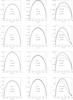Fig. 2 Dependence of the dimensionless instability increment σ on the ratio of the wavenumber to the critical wavenumber κ/κc for four particular values of the angles α and φ. The left, middle, and right panels correspond to β = 5, 1, and 0.01, respectively. The solid, dashed, and dash-dotted curves correspond to ν = 10-4, 0.1, and 1, respectively. In the left panels all the curves are indistinguishable. In the middle panels the solid and dashed curves are indistinguishable.

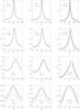Fig. 3 Dependence of the maximum with respect to κ of the dimensionless instability increment, σm, on the angle φ. The left, middle, and right panels correspond to β = 5, 1, and 0.01, respectively. The solid, dashed, and dash-dotted curves correspond to ν = 10-4, 0.1, and 1, respectively. In the panels where one single curve is plotted all the curves are indistinguishable.

When solving the dispersion equation Eq. (56) numerically we consider ζ = 100 and χ = 1. Then it follows from Eq. (45) that β₁ = β₂ = β. We now estimate the dimensionless coefficient of ambipolar diffusion ν. For typical values of the prominence plasma we take ρ₂ = 10^-10 kgm^-3, c_A2 = 100 km s^-1, g = 274 m s^-2, and the plasma temperature 10⁴ K. Then, taking into account that the prominence plasma is only weakly ionised and ξ_n ≈ 1, we obtain 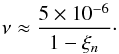$\mathit{\nu }\mathrm{\approx }\frac{\mathrm{5}\mathrm{\times }{\mathrm{10}}^{-6}}{\mathrm{1}\mathrm{-}{\mathit{\xi }}_{\mathit{n}}}\mathrm{·}$(71)The above relation shows that unless the plasma is extremely weakly ionised, ν ≪ 1. We calculated the dependence of the instability increment σ on κ for various values of β, α, and φ, and for ν = 10^-4, 0.1, and 1, which corresponds to 1−ξ_n = 0.05, 5 × 10^-5, and 5 × 10^-6. The results of this calculation are shown in Fig. 2. These plots show that when β = 5, which is very close to the limit of incompressible plasma, the three curves are indistinguishable and the maximum instability increment is obtained for κ/κ_c ≈ 0.5. The result obtained in this case confirms the conclusion that, in the limit of incompressible plasma, the ambipolar diffusion does not affect the MRT instability. We verified that for all values of β, α, and φ the solid curves corresponding to ν = 10^-4 are the same as those obtained in the approximation of ideal MHD. Hence, we can conclude that even when the prominence plasma is relatively weakly ionized with only one proton per 20 hydrogen atoms the effect of ambipolar diffusion on the appearance of the MRT instability at the interface between the prominence and corona is almost negligible.

In general, we see that the ambipolar diffusion reduces the instability increment and the maximum increment is obtained for smaller wavenumbers (larger wavelengths) as the number of neutrals is increased. For small values of plasma beta (as in the case of prominences) the decrease in the increment for ν = 1 can be up to 40%. Nevertheless, even for these values of plasma beta, noticeable reduction in the instability increment occurs when the prominence plasma is extremely weakly ionised, with the ratio of number of neutral hydrogen atoms to the number of ions of the order of 10⁵.

We also study the dependence on φ of the maximum instability increment with respect to κ, and the dependence on α of the maximum instability increment with respect to κ and φ. These two quantities are defined by ${\mathit{\sigma }}_{\mathrm{m}}\mathrm{=}\underset{\mathit{\kappa }}{\max }\mathit{\sigma ,} {\mathit{\sigma }}_{\mathrm{M}}\mathrm{=}\underset{\mathit{\kappa ,}\hspace{0.17em}\mathit{\phi }}{\max }\mathit{\sigma }\mathit{.}$(72)The results of our calculations are shown in Figs. 3 and 4. In Fig. 3, we see that the effect of ambipolar diffusion becomes stronger when α increases and β decreases. Again, a significant variation in the instability increment occurs for β ≪ 1, i.e. for the prominence and upper chromospheric conditions. We also see that the maximum increment occurs when the wave vector is almost perpendicular to the ambient magnetic field in the prominence. When β ≪ 1 the increment decreases with the increase in the number of neutrals in the plasma. The value of σ_m is almost independent of φ and close to 0.5 when α = 90° and β = 5. This result agrees very well with the fact that, in the approximation of incompressible plasma, σ_m = 0.5 when α = 90°. We also verified that the solid curves corresponding to ν = 10^-4 almost coincide with the similar curves obtained by Ruderman (2017) in the approximation of ideal MHD.

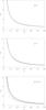Fig. 4 Dependence of the maximum with respect to κ and φ of the dimensionless instability increment, σM, on the angle α. The upper, middle, and lower panels correspond to β = 5, 1, and 0.01, respectively. The solid, dashed, and dash-dotted curves correspond to ν = 10-4, 0.1, and 1, respectively. In the upper and middle panels all the curves are indistinguishable.

We verified that the solid curves in Fig. 4 corresponding to ν = 10^-4 coincide with the similar curves obtained by Ruderman (2017) in the approximation of ideal MHD. Figure 4 also reveals that the ambipolar diffusion only affects the maximum growth rate σ_M when the plasma beta is very small and, in addition, the prominence plasma is extremely weakly ionised. This conclusion is important for applications to the prominence seismology. Following the assumption by Terradas et al. (2012) that the prominence disappearance evident from the observational results reported by Okamoto et al. (2007) was caused by the MRT instability, Ruderman et al. (2014) estimated the shear angle α between the magnetic field in the prominence and in the surrounding coronal plasma. When doing so they used the results obtained in the approximation of incompressible plasma. Ruderman (2017) extended this analysis to include the plasma compressibility and also applied it to observations of the MRT instability in prominences reported by Ryutova et al. (2010). He found that the account of plasma compressibility does not affect the estimates of α. On the basis of the results obtained in this article we can make the same conclusion about the effect of ambipolar diffusion. The values of σ_M in Fig. 4 do not reach a maximum value, instead their evolution towards smaller shear angle was cut because σ_M → ∞ as α → 0.

5. Conclusions

The present study deals with the problem of the magnetic Rayleigh-Taylor instability in partially ionised compressible plasmas in the presence of magnetic shear, meaning that the equilibrium magnetic field has different directions below and above the magnetic interface. The dynamics of the plasma was described within the framework of single-fluid MHD, and the effect of partial ionisation appeared in the induction equation in the form of ambipolar diffusion. The magnitude of the dissipative coefficient is determined by the amount of neutrals in the fluid.

First of all, our analysis demonstrated that the MRT instability only appears for wavenumbers that are smaller than a critical cut-off value. This value is determined by the density and magnetic field contrasts between the two regions, by the angle between the wave vector of a perturbation and the equilibrium magnetic field, and by the degree of magnetic shear. However, this critical wavenumber is independent of the plasma beta and ionisation degree of the plasma. Hence, fully and partially ionised plasmas have the same critical wavenumber. We need to mention here that the existence of the critical wavenumber is very much connected to the equilibrium chosen for our model. Díaz et al. (2014) and Khomenko et al. (2014) studied the MRT instability of a magnetic interface with the plasma only partially ionised at both sides. They found that for such an equilibrium there is no critical wavenumber meaning that perturbations with any wavenumber are unstable. Hence, the existence of the critical wavenumber is related to the assumption that the plasma is fully ionised at one side of the magnetic interface.

In the incompressible limit the ambipolar diffusion does not affect the evolution of the instability. This result is further confirmed by our numerical investigation for high values of plasma beta. When the plasma beta is large the curves showing the dependence of the maximum increment σ_M on the magnetic shear angle α and corresponding to different degrees of ionisation practically coincide (see Fig. 4). Our investigation showed that a significant dependence of the maximum instability increment on the ionisation degree only occurs in the β ≪ 1 regime, where the decrease in the increment can be as large as 40% for the values of parameters considered here.

There is a simple physical explanation why the ambipolar diffusion does not affect the maximum increment of the MRT instability in the approximation of incompressible plasma corresponding to β → ∞. Ambipolar diffusion appears because the neutrals and ions have different velocities. This velocity difference, in turn, appears because the Lorentz force affects the motion of ions and does not affect the motion of neutrals. In the limit of β → ∞ the Lorentz force is negligible in comparison with the pressure gradient. As a result, the ions and neutrals move with the same velocity and the effect of ambipolar diffusion disappears. When β is finite but large the velocities of ions and neutrals do not coincide; however, their difference is very small and, consequently, the effect of ambipolar diffusion is also very small. Our calculations show that this effect is actually very small even when β is of the order of unity. It only becomes substantial when β ≪ 1.

The value of β also affects the maximum value of the increment; this maximum value decreases when β decreases while the values of propagation angle and magnetic shear are fixed. The increment takes its maximum when the wave vector of a perturbation is almost perpendicular to the magnetic field in the dense plasma. It is only affected by the ionisation degree when this degree is extremely small and, in addition, β is small.

We note that in the numerical investigation of the dispersion equation we always took β₁ = β₂ = β. If we make a viable assumption that β₂ ≳ 1 when β₁ ≳ 1, then ambipolar diffusion does not affect the maximum instability increment for any values of β₂/β₁. On the other hand, the maximum increment becomes independent of β₁ and β₂ when both these quantities are smaller than or of the order of 0.01. For these small values of β₁ and β₂ it is very nearly equal to its limiting value obtained when β₁ → 0 and β₂ → 0.

Acknowledgments

This study was initiated when M.S.R. visited the Instituto de Astrofísica de Canarias (IAC). He thanks IAC for their warm hospitality. The authors acknowledge the financial support by the Leverhulme Trust (IN-2014-016). M.S.R. also acknowledges the support by STFC. I.B. was partly supported by a grant of the Ministry of National Education and Scientific Research, RDI Programme for Space Technology and Advanced Research – STAR, project number 181/20.07.2017.

References

Appendix A: Investigation of Eq. (46)

In this section we show that Eq. (46) has exactly two positive roots when σ> 0. We rewrite Eq. (46) as ${\mathit{f}}_{\mathrm{1}}\mathrm{\left(}\mathrm{\Lambda }\mathrm{\right)}\mathrm{=}{\mathit{f}}_{\mathrm{2}}\mathrm{\left(}\mathrm{\Lambda }\mathrm{\right)}\mathit{,}$(A.1)where $\begin{array}{ccc}{\mathit{f}}_{\mathrm{1}}\mathrm{\left(}\mathrm{\Lambda }\mathrm{\right)}& \mathrm{=}& \\ {\mathit{f}}_{\mathrm{2}}\mathrm{\left(}\mathrm{\Lambda }\mathrm{\right)}& \mathrm{=}& \mathrm{[}{\mathit{\sigma }}^{\mathrm{2}}\mathrm{(}\mathrm{1}\mathrm{+}{\mathit{\beta }}_{\mathrm{2}}\mathrm{)}\mathrm{+}{\mathit{\beta }}_{\mathrm{2}}{\mathit{\kappa }}^{\mathrm{2}}{\cos }^{\mathrm{2}}{\mathit{\phi }}^{\mathrm{]}}{\mathrm{\Lambda }}^{\mathrm{2}}\\ & & \end{array}$and Λ = Λ_j. It is straightforward to see that the equation f₁(Λ) = 0 has exactly two positive and two negative roots, and the equation f₂(Λ) = 0 has exactly one positive and one negative root. Typical graphs of functions f₁(Λ) and f₂(Λ) are shown in Fig. A.1. We note that the mutual positions of negative zeros of functions f₁(Λ) and f₂(Λ) can be different from those shown in Fig. A.1. However, this fact is not important because we are only interested in the positive roots of Eq. (46). The smaller positive zero of function f₁(Λ) is κ, while the larger positive zero is ${\mathrm{\Lambda }}_{\mathrm{0}}\mathrm{=}\frac{\mathrm{1}\mathrm{+}\sqrt{\mathrm{1}\mathrm{+}\mathrm{4}{\mathit{\beta }}_{\mathrm{2}}\left({\mathit{\sigma }}^{\mathrm{2}}\mathrm{+}{\mathit{\beta }}_{\mathrm{2}}{\mathit{\kappa }}^{\mathrm{2}}\right)}}{\mathrm{2}{\mathit{\beta }}_{\mathrm{2}}}\mathrm{·}$(A.4)We denote the positive zero of function f₁(Λ) as Λ₊ and prove that κ< Λ₊< Λ₀. We have f₂(κ) = −σ²κ< 0, which implies

that κ< Λ₊. After straightforward calculation we obtain that the inequality f₂(Λ₀) > 0 is equivalent to the obvious inequality $\sqrt{\mathrm{1}\mathrm{+}\mathrm{4}{\mathit{\beta }}_{\mathrm{2}}\left({\mathit{\sigma }}^{\mathrm{2}}\mathrm{+}{\mathit{\beta }}_{\mathrm{2}}{\mathit{\kappa }}^{\mathrm{2}}\right)}\mathrm{+}\mathrm{1}\mathrm{+}\mathrm{2}{\mathit{\beta }}_{\mathrm{2}}{\mathit{\sigma }}^{\mathrm{2}}\mathit{>}\mathrm{0.}$(A.5)The inequality f₂(Λ₀) > 0 implies that Λ₊< Λ₀. This inequality implies that the graphs of functions f₁(Λ) and f₂(Λ) have two points of intersection for Λ > 0 meaning that Eq. (46) has exactly two positive roots.

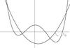Fig. A.1 Graphical investigation of Eq. (A.1). The curve with four zeros is the graph of function f1(Λ), while the curve with two zeros is the graph of function f2(Λ).

All Figures

	Fig. 1 Sketch of the equilibrium. The interface at z = 0 separates the fully ionised solar corona (region 1) and the partially ionised prominence (region 2).
In the text

Fig. 2 Dependence of the dimensionless instability increment σ on the ratio of the wavenumber to the critical wavenumber κ/κc for four particular values of the angles α and φ. The left, middle, and right panels correspond to β = 5, 1, and 0.01, respectively. The solid, dashed, and dash-dotted curves correspond to ν = 10-4, 0.1, and 1, respectively. In the left panels all the curves are indistinguishable. In the middle panels the solid and dashed curves are indistinguishable.

In the text

	Fig. 3 Dependence of the maximum with respect to κ of the dimensionless instability increment, σm, on the angle φ. The left, middle, and right panels correspond to β = 5, 1, and 0.01, respectively. The solid, dashed, and dash-dotted curves correspond to ν = 10-4, 0.1, and 1, respectively. In the panels where one single curve is plotted all the curves are indistinguishable.
In the text

	Fig. 4 Dependence of the maximum with respect to κ and φ of the dimensionless instability increment, σM, on the angle α. The upper, middle, and lower panels correspond to β = 5, 1, and 0.01, respectively. The solid, dashed, and dash-dotted curves correspond to ν = 10-4, 0.1, and 1, respectively. In the upper and middle panels all the curves are indistinguishable.
In the text

	Fig. A.1 Graphical investigation of Eq. (A.1). The curve with four zeros is the graph of function f1(Λ), while the curve with two zeros is the graph of function f2(Λ).
In the text

References

- Bommier, V., Landi Degl’Innocenti, E., Leroy, J. L., & Sahal-Brechot, S. 1994, Sol. Phys., 154, 231 [NASA ADS] [CrossRef] [Google Scholar]
- Bucciantini, N., Amato, E., Bandiera, R., Blondin, J. M., & Del Zanna, L. 2004, A&A, 423, 253 [NASA ADS] [CrossRef] [EDP Sciences] [Google Scholar]
- Díaz, A. J., Khomenko, E., & Collados, M. 2014, A&A, 564, A97 [NASA ADS] [CrossRef] [EDP Sciences] [Google Scholar]
- Hilier, A., Isobe, H., Shibata, K., & Berger, T. 2011, ApJ, 736, L1 [NASA ADS] [CrossRef] [Google Scholar]
- Hilier, A., Berger, T., Isobe, H., & Shibata, K. 2012a, ApJ, 746, 120 [NASA ADS] [CrossRef] [Google Scholar]
- Hilier, A., Isobe, H., Shibata, K., & Berger, T. 2012b, ApJ, 756, 110 [NASA ADS] [CrossRef] [Google Scholar]
- Isobe, H., Miyagoshi, T., Shibata, K., & Yokoyama, T. 2005, Nature, 434, 478 [NASA ADS] [CrossRef] [Google Scholar]
- Isobe, H., Miyagoshi, T., Shibata, K., & Yokoyama, T. 2006, PASJ, 58, 423 [Google Scholar]
- Jones, T. W., & De Young, D. S. 2005, ApJ, 624, 586 [NASA ADS] [CrossRef] [Google Scholar]
- Jun, B.-I., & Norman, M. L. 1996, ApJ, 472, 245 [NASA ADS] [CrossRef] [Google Scholar]
- Jun, B.-I., Norman, M. L., & Stone, J. M. 1995, ApJ, 453, 332 [NASA ADS] [CrossRef] [Google Scholar]
- Khomenko, E., Díaz, A. J., de Vicente, A., Collados, M., & Luna, M. 2014, A&A, 565, A45 [NASA ADS] [CrossRef] [EDP Sciences] [Google Scholar]
- Leroy, J. L., Bommier, V., & Sahal-Brechot, S. 1984, A&A, 131, 33 [Google Scholar]
- Okamoto, T. J., Tsuneta, S., Berger, T. E., et al. 2007, Science, 318, 1577 [NASA ADS] [CrossRef] [PubMed] [Google Scholar]
- O’Neil, M., Alouani Bibi, F., Toth, J., et al. 2009, Nature, 462, 1036 [NASA ADS] [CrossRef] [PubMed] [Google Scholar]
- Robinson, D., Dursi, L. J., Ricker, P. M., et al. 2004, ApJ, 601, 621 [NASA ADS] [CrossRef] [Google Scholar]
- Ruderman, M. S. 2015, A&A, 580, A37 [NASA ADS] [CrossRef] [EDP Sciences] [Google Scholar]
- Ruderman, M. S. 2017, Sol. Phys., 292, 47 [NASA ADS] [CrossRef] [Google Scholar]
- Ruderman, M. S., Terradas, J., & Ballester, J. L. 2014, ApJ, 785, A110 [NASA ADS] [CrossRef] [Google Scholar]
- Ryutova, M. P., Berger, T., Frank, Z., Tarbell, T., & Title, A. 2010, Sol. Phys., 267, 75 [Google Scholar]
- Terradas, J., Oliver, R., & Ballester, J. L. 2012, A&A, 541, A102 [NASA ADS] [CrossRef] [EDP Sciences] [Google Scholar]