| Issue |
A&A
Volume 606, October 2017
|
|
|---|---|---|
| Article Number | A67 | |
| Number of page(s) | 8 | |
| Section | Stellar structure and evolution | |
| DOI | https://doi.org/10.1051/0004-6361/201731639 | |
| Published online | 12 October 2017 | |
The photodissociation of CO in circumstellar envelopes ⋆
Koninklijke Sterrenwacht van België, Ringlaan 3, 1180 Brussels, Belgium
e-mail: This email address is being protected from spambots. You need JavaScript enabled to view it.
Received: 25 July 2017
Accepted: 9 August 2017
Abstract
Carbon monoxide is the most abundant molecule after H2 and is important for chemistry in circumstellar envelopes around late-type stars. The size of the envelope is important when modelling low-J transition lines and deriving mass-loss rates from such lines. Now that ALMA is coming to full power the extent of the CO emitting region can be measured directly for nearby asymptotic giant branch (AGB) stars. In parallel, it has become obvious in the past few years that the strength of the interstellar radiation field (ISRF) can have a significant impact on the interpretation of the emission lines. In this paper an update and extension of the classical Mamon et al. (1988, ApJ, 328, 797) paper is presented; these authors provided the CO abundance profile, described by two parameters, as a function of mass-loss rate and expansion velocity. Following recent work an improved numerical method and updated H2 and CO shielding functions are used and a larger grid is calculated that covers more parameter space, including the strength of the ISRF. The effect of changing the photodissociation radius on the low-J CO line intensities is illustrated in two cases.
Key words: astrochemistry / stars: AGB and post-AGB / stars: winds, outflows / radio continuum: stars
Full Table 1 is only available at the CDS via anonymous ftp to cdsarc.u-strasbg.fr (130.79.128.5) or via http://cdsarc.u-strasbg.fr/viz-bin/qcat?J/A+A/606/A67
© ESO, 2017
1. Introduction
Nearly three decades ago Mamon et al. (1988, hereafter MGH) published a paper with the same title as the present paper. These authors calculated the unshielded CO photodissociation rate (I0 = 2.0 × 10⁻¹⁰ s-1), and found it to be a factor 10 larger than earlier studies used at the time (2 × 10-11 s-1; Federman et al. 1980). Mamon et al. used a schematic one-dimensional model to calculate the CO distribution in the envelopes around evolved stars. This distribution was approximated by a two-parameter model (see Eq. (7)), and the parameters were given in tabular form as a function of a range of mass-loss rates and three expansion velocities. Very quickly, several analytical fit formulae to this tabular data were presented (Planesas et al. 1990; Kwan & Webster 1993; Stanek et al. 1995).
The original MGH results and the analytical formulae are still widely in use today to estimate qualitatively the size of the CO shell and whether such a shell would be resolved by a single-dish radio telescope. The MGH results are also used in molecular radiative transfer (RT) codes to fix the CO abundance profile as a function of distance to the central star for a given (assumed) mass-loss rate and expansion velocity.
Almost 30 yr later it seems timely to revisit the problem. The unshielded CO photodissociation rate has been revised upwards by about 30% (Visser et al. 2009) and detailed shielding functions are available (Visser et al. 2009). The MGH study used some analytical approximations for the two-dimensional problem in the calculation of the shielded photodissociation rate as a function of distance to the star. These approximations are not needed and the two-dimensional problem can be solved numerically (Li et al. 2014). On the observational side, the ALMA interferometer is reaching its full potential, and CO envelopes can be studied in much more detail. The spatial extent of the molecular shells of nearby evolved stars can be determined accurately, and therefore detailed theoretical predictions of the size of the CO shell seem timely.
Li et al. (2014, 2016) recently incorporated the shielding functions by Visser et al. (2009) and the N2 shielding function (Li et al. 2013) together with a numerical integration scheme (dubbed “the spherically symmetric model”) into a chemical network code to calculate abundance profiles for various molecules in the envelopes around IK Tau and CW Leo. This model and the CO shielding functions are at the basis of the present work.
It has also become clear in recent years that the strength of the radiation field plays an important role. The MGH work used the interstellar radiation field (ISRF) by Jura (1974), calculated for the solar vicinity by explicitly considering the Sun and 14 stars earlier than B5 listed in the Catalogue of Bright Stars. At the five wavelengths between 930 and 1125 Å listed by Jura the ISRF by Draine (1978) agrees to within 5%. Draine also provides estimates for the ISRF above the Galactic plane and, for a range of parameters, typical strengths are between 0.2 and 0.8 times the value in the Galactic plane.
Doty & Leung (1998) considered the effect of the strength of the ISRF in their model of the envelope around IRC +10° 216 (CW Leo). Their results are a bit difficult to estimate (see one of the tiny panels in their Fig. 8) but suggest a decrease in the photodissociation radius by a factor of ~4 when increasing the strength of the ISRF by a factor of 9.
McDonald et al. (2015) presented the results of ALMA observations of evolved stars in the globular cluster 47 Tucanae. Four of the brightest AGB stars with estimated mass-loss rates of a few 10-7M⊙ yr-1 based on their infrared emission were observed in the CO J = 2 − 1 line. None of these stars were detected although the observations were sensitive enough to detect line strengths predicted by standard formulae (Olofsson 2008; and Ramstedt et al. 2008, for details) based on observations of a range of Galactic AGB stars. McDonald et al. (also see McDonald & Zijlstra 2015) estimated the ISRF to be typically 50 times stronger than the Galactic ISRF, depending om the location of the star in the cluster and other factors, but stronger than a factor of 2.5 with a probability of at least 85% for all four objects. McDonald et al. also estimated that the CO envelopes were truncated at a few hundred stellar radii and that the line intensities were about two orders of magnitude below their current detection limits. These authors also found the radiation field to be harder than the Draine field. Zhukovska et al. (2015) showed the importance of the ISRF in the photodissociation of SiO in clusters. These authors found that AGB stars in clusters experience an ultraviolet (UV) field typically 10−100 times the ISRF. Groenewegen et al. (2016) discussed the non-detection of CO J = 2 − 1 in one and the marginal detection in another OH/IR star in the LMC. There are several possible reasons for this, but one is the stronger radiation field in the LMC diffuse medium by a factor of ~5 (Paradis et al. 2009) compared to the Galactic Draine field.
In Sect. 2 the physical problem and the mathematical and numerical solution to this problem are presented. The calculations are presented in Sect. 3 and discussed in Sect. 4. Section 5 concludes this paper.
2. Equations and solutions
Consider a spherically symmetric homogeneous outflow with expansion velocity V. If photodissociation is the only destruction mechanism and in the absence of molecular formation processes, the number density, n, of CO is given by (Jura & Morris 1981) 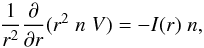 (1)with I the photodissociation rate. Using (r2nV) as variable, the solution of the CO abundance relative to H2, and relative to the value at the inner radius, for constant velocity is
 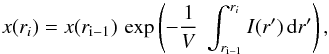 (2)with the boundary condition that at the inner radius x(r1) = 1. In the case of unshielded radiation, I(r) = I0, and the solution becomes
 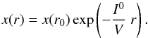 (3)The shielded dissociation rate at a point in the envelope depends on the conditions in the entire shell
 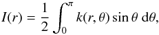 (4)where k(r,θ) is the dissociation rate at a radius r from the central star by interstellar photons along a ray making an angle θ (Li et al. 2014, see Fig. A.1).
The integration over θ effectively goes from 0 to (π − β), where  (5)indicates the angle subtended by the central star (or the inner radius of the envelope) from point ri. The UV radiation field from the cool AGB can be neglected. The numerical code could be adapted however to include the radiation from a hotter central object, simulating either a corona or chromosphere around the central star or a close binary component. This would make the problem time dependent however.
The dissociation rate can be written as (Li et al. 2014)  (6)where I0 = 2.6 × 10⁻¹⁰ s-1 (Visser et al. 2009) is the unshielded photodissociation rate, χ is a scaling factor indicating the strength of the ISRF relative to the Draine (1978) field adopted in Visser et al., and Θdust = exp ( − τdust) the shielding by dust and ΘH2,CO the 12CO self-shielding and shielding by H2 and the CO isotopologues (Visser et al. 2009). The tabulated shielding function in Visser et al. depend on the CO and H2 column density, and the excitation temperature1.
This immediately implies that the solution to Eq. (2) must be obtained by iteration, as the CO photodissociation rate in a point in the circumstellar envelope (CSE) depends on the CO column density along all rays (see Fig. A.1). The solution proceeds as follows (following Li et al.):
-
Assume a CO profile in the envelope. Theparametrisation introduced by MGH is used, i.e.
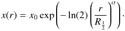 (7)
(7) -
In point ri determine the column densities of CO and H2 (see Appendix A) and the dust optical depth along all angles, and perform the integration over θ.
-
With I(ri) determined, calculate x(ri) from Eq. (2), and proceed to the next radial point.
-
After the full profile is determined, fit Eq. (7) to it, and determine new estimates for
 and α. Iterate until these two parameters no longer
change.
and α. Iterate until these two parameters no longer
change.
 ) (Eq. (A.3)). In other codes the prescription of the dust extinction is more general, for example Li et al. (2014) essentially used the H2 column density and a standard conversion factor (Bohlin et al. 1978; Rachford et al. 2009) to determine the extinction. Mamon et al. and others (Nejad & Millar 1987; Doty & Leung 1998) typically assumed an optical depth in the UV at a given inner radius (Eq. (A.4)), which scales with the assumed mass-loss rate and velocity (Eq. (A.3)). Doty & Leung (1998) found that for parameters typical for CW Leo a change in dust optical depth by a factor of five has a very small effect on the CO profile.
Less important parameters are the inner radius of the shell, where the calculation starts – a few stellar radii, where the stellar radius is determined from the stellar luminosity and the effective temperature of the central star, which are input parameters–and the outer radius, which is arbitrarily set to 15 . In the limiting case of α → 1 for very low mass-loss rates the relative abundance has dropped to ~3 × 10⁻⁵ at that distance.
Finally, the CO excitation temperature profile needs to be provided. The MGH study took a gas kinetic temperature profile that is derived for CW Leo and assume this profile is valid in all their calculations. These authors assumed that the excitation temperature equals the gas temperature, and for parameters typical for CW Leo test the case that the excitation temperature is half the gas temperature finding that is increased by ~20%. Doty & Leung (1998) found that for parameters typical for CW Leo, a factor of two change in gas temperature has a small effect on the CO abundance profile. Li et al. (2014), in their model for CW Leo, took the excitation temperature to be constant in the CSE and equal to 5 K, as they found that CO is subthermally excited at the low densities in the outer parts of the CSE. The CO models for OH 32.8−0.3 and OH 44.8−2.3 (Groenewegen 1994b), the halo carbon star IRAS 12560+1657 (Groenewegen et al. 1997), and CW Leo (Groenewegen et al. 1998) indeed show this to be the case. In these models, the excitation temperatures of the J = 1 − 0 to 4−3 transitions range from 3 to 12 K in the regions of the wind where the CO abundance has dropped to ~0.8 to ~0.3 of its initial value, and the excitation temperatures are always lower, and sometimes lower by a factor of a few, than the gas temperature at these radii. Additional details on the calculations are provided in Appendix A.
3. Calculations
A large model grid was calculated using the following parameters:
-
Seventeen mass-loss rates (MLRs) between1 × 10-13 and 2 × 10⁻⁴M⊙ yr-1. The lowest MLR could never be measured in practice but allows a numerical check of the results in the case of unshielded radiation.
-
Expansion velocities of 3.0, 7.5, 15 and 30 km s-1.
-
Nine CO abundances between 0.1 × 10⁻⁴ and 12 × 10-4.
-
Nine different strengths of the ISRF, χ = 0.01, 0.1, 0.2, 0.5, 1, 2, 5, 10, and 100.
-
Four constant excitation temperatures of 5, 20, 50, and 100 K.
and α are given in Table 1, which is available in its entirety at the CDS. Not all possible combinations are listed in the Table. For the lowest MLRs and the largest ISRF strengths the calculated dissociation radius is smaller than the adopted inner radius. In Table 1 selected models are listed to illustrate the general behaviour of the results. The models are for standard values of fCO = 8 × 10⁻⁴, expansion velocity 15 km s-1, standard ISRF, and excitation temperature of 5 K. The table also lists the results when changing these parameters. The values found by MGH are listed for comparison for the various MLRs. A value of 1 × 10⁻⁵M⊙ yr-1 is the standard value considered in the discussion below. The standard value for MLR, CO abundance and expansion velocity adopted here are the same as in the standard model in MGH.
For the standard model, Table 1 lists the result when changing the dust properties by a factor of 3 (an effect of  on ) and using CO shielding functions for a different assumed Doppler width or isotopic abundance ratio (see Visser et al. 2009), with an ~1% effect.
CO line profile parameters and α as a function of input parameters.
4. Discussion
4.1. No mass loss
In the limit of very low mass-loss rates, that is essentially unshielded radiation, Eqs. (3) and (7) show that one expects α → 1 and  . The typical radius for the abundance to change in the unshielded Draine ISRF is therefore 4.0 × 1015 cm in an envelope with 15 km s-1 expansion velocity.
Inspection of Table 1 shows that α indeed is close to unity in the models with the lowest mass-loss rates, but that is larger than the expected values. This is the effect of the finite R⋆ and Rin adopted in the models. It implies that some of the ISRF is blocked by the central star and that the photodissociation radius is therefore slightly larger.
Table 1 includes a model with an even lower MLR (1 × 10-15M⊙ yr-1), models were the stellar radius is systematically decreased (by lowering the stellar luminosity), and a model in which Rin is decreased from 4 to 1.1 R⋆. The half-radius and α indeed converge to the expected values in the limiting case of unshielded radiation.
4.2. Comparing to MGH
Table 1 lists the results found here and those listed in MGH. The behaviour is complicated. For the lowest MLRs the value for found here is typically a factor of about 2 larger, but the difference becomes smaller with increasing MLR and the values are about equal near 2 × 10⁻⁵M⊙ yr-1.
The main difference in the two approaches is in the way the shielding is calculated, but there are other differences. Therefore an attempt was made to more closely follow the assumptions made in MGH.
Mamon et al. assumed that the CO excitation temperature follows the gas kinetic temperature, and their temperature law was adopted here. The default dust properties were changed to give the dust optical depth at 1000 Å adopted by MGH. The inner radius is set at 1016 cm and the central star is assumed to be a point source. The ISRF adopted in MGH is different from adopted here; the field as determined by Jura et al. (1974) implies χ = 0.77 with respect to the Draine field.
In our model, the resulting value for is larger than in the standard model by about 7% and is 22% larger than MGH. The difference between the use of “the spherically symmetric model” compared to the one-dimensional approach in MGH is difficult to quantify (but see Li et al. 2014). This implies that the shielding in Visser et al., which included updated molecular data compared to MGH, is more effective than in the older approach.
Figure 1 compares the dissociation rate of the standard model with MGH (their Fig. 1). The rate is indeed larger, leading to a smaller photodissociation radius. Figure 2 shows the relative CO abundance in the envelope for the standard model and compares this model to the MGH model (see their Fig. 2), while Fig. 3 shows the profile for several MLRs (cf. Fig. 3 in MGH).
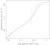 |
Fig. 1 Solid lines indicates the CO photodissociation rate as a function of radial distance for the standard model. The dashed line indicates the value of |
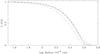 |
Fig. 2 Solid line indicates the relative CO profile for the standard model, while the dashed line gives the profile for the fitted values of |
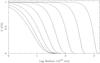 |
Fig. 3 CO abundance profiles for MLRs between 10-11 and 10-4M⊙ yr-1 in steps of a decade. |
4.3. Fitting formula
Soon after the publication of MGH, several convenient fitting formulae were published that allowed the community to estimate and α for a large parameter space. The formula in Planesas et al. (1990) is 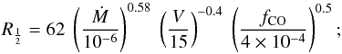 (8)Kwan & Webster (1993) derived
 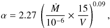 (9)and (for the value of fCO = 8 × 10⁻⁴ assumed by MGH)
 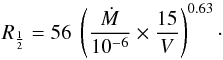 (10)The most elaborate approximation formula is that by Stanek et al. (1995), who considered the analytical value in the limit of small mass loss rates,
 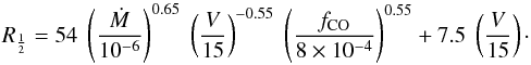 (11)This functional form is used here as well and the fit is shown in Eq. (12). This fit was derived as follows. The second term on the right-hand side is the value in the limit of unshielded radiation and has an analytic result, where a correction was applied because of the finite size of the central star; see Sect. 4.1 (fsc = 4.144 / 4 = 1.036; see Table 1). This term was subtracted from the calculated value of and then a multi-dimensional linear fit in logarithmic space was made using the SVDFIT routine available in Numerical Recipes (Press et al. 1992). The fit was restricted to models with MLRs larger than 10-8M⊙ yr-1 and 0.1 <χ< 10. In addition models with velocities of 3.0 km s-1 were excluded for MLRs larger than 5 × 10⁻⁵M⊙ yr-1; these models showed larger residuals and in fact such combinations of parameters are not observed. Similarly, Eq. (13) shows the fit for α, i.e.
 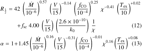 Although the fitting formula may be convenient, it is definitely recommended to interpolate in Table 1 directly. The uncertainty in the power law fit is important; i.e. to have the fitting routine return a reduced χ2 of unity, an uncertainty of about 24% in and about 11% in α had to be assigned.
The dependence on velocity and CO abundance is generally weaker compared to the fits in the literature. The dependence on the excitation temperature is small. Of most interest is the dependence on the strength of the ISRF. Globally, a factor of 15 increase in the ISRF leads to a photodissociation radius that is three times smaller.
4.4. The effect in two cases
As an illustration, the effect of the new photodissociation radii on the CO line intensities is considered in two cases: the peculiar OH/IR star OH 32.8−0.3, and the star V1 in the cluster 47 Tucanae, which were fitted using the model in Groenewegen (1994a). It is not the aim here to re-derive the MLRs, but only to show the typical effect a change in photodissociation radius may have. A full modelling of an individual star would also consider the line shape of the lines, but here only integrated line intensities are compared.
Table 2 lists the default stellar parameters adopted in Groenewegen (1994b) and McDonald et al. (2015) for OH 32.8 and 47Tuc V1, respectively. Table 3 lists the observed data in the first row (see below), and then the model results, where the second row gives the result for the photodissociation radii based on MGH.
Sample of stars.
CO model results.
4.4.1. OH 32.8−0.3
For OH 32.8−0.3 (V1365 Aql, IRAS 18498-0017) the CO(1−0) and (2−1) data are listed that were taken in the 23 and 11.3′′ beam of the IRAM 30 m telescope and fitted in Groenewegen (1994b). In addition, more recent data in the J = 3 − 2 and 4−3 lines are listed for both stars, taken from De Beck et al. (2010). The data are taken with the JCMT in beams of 14′′ and 11′′, respectively. No error bars were provided.
This star comes from the “Group 2” objects defined by Heske et al. (1990). In the objects, the MLR based on the CO(1−0) and (2−1) lines is much smaller than that based on the dust, either using the IRAS 60 μm flux as a tracer, as in Heske et al., or from dust RT modelling of the spectral energy distribution (SED), as in Groenewegen (1994b). This is clear from the first entries in Table 3. The J = 1 − 0 flux is 10 times stronger then the observed upper limit. Even if the new photodissociation radius is significantly smaller than the value deduced from MGH the discrepancy remains.
The subsequent models are calculated for a lower MLR, but increasing the dust-to-gas ratio, so that the dust MLR, derived from modelling the SED, remains constant. The predicted line intensities are lower, but still too large. Also the dust-to-gas ratio becomes large at 1/50, i.e. larger than the typically assumed value in the local interstellar medium. The next entry is for a model in which the distance is decreased; in fact this model is tuned to fit the observed J = 3 − 2 and 4−3 data. However the J = 1 − 0 and 2−1 data are overestimated by factors 3−5.
One possible option to decrease the flux is an increased ISRF, which would make the envelope smaller. Table 3 lists the results for χ = 2 and the value of 50 that is required to predict J = 1 − 0 and 2−1 intensities in reasonable agreement with observations. The J = 3 − 2 intensity is however now also lower than observed. It is beyond the scope of the paper to assess the likelihood of this scenario. However, it would suggest that OH 32.8 is located in or close to a cluster.
An alternative scenario, which was considered in Groenewegen (1994b), is that the MLR is not constant. Groenewegen (1994b) considered a MLR a factor 10 lower for radial distances larger than 1017 cm, corresponding to a timescale of about 2000 yr. Such a model is considered in the last two entries. In one entry, the photodissociation radius was based on the current MLR; in the second entry, the molecular hydrogen density was also lowered for radial distances larger than 1017 cm and the shielding and resulting CO abundance profile was calculated in a consistent way in the photodissociation model. In this case the latter improvement does not have an important effect and the J = 1 − 0 and 2−1 data can be explained by such a model. In fact the model with a sharp drop in MLR, and the model with a much stronger ISRF predict indistinguishable line intensities. The models also show that the J = 4 − 3 and higher transitions are little affected by such extreme models.
4.4.2. 47 Tuc V1
The model for the variable star V1 in 47 Tuc is unpublished. It was created in connection with McDonald et al. (2015), of which MG is a co-author, but the results were not included there; that paper discusses the results from two other models. The observed data point is the non-detection of the J = 2 − 1 line in an ALMA beam of 2′′. The model for the 1−0, 3−2, 4−3, and 6−5 data are calculated in beams of 4, 1.3, 1, and 0.33′′. An expansion velocity of 10 km s-1 is adopted.
The models in Table 3 show the result for increasing strength of the ISRF. For a standard ISRF one would have expected 7−10σ detections, which was the original premise of performing the ALMA observations. A value of χ = 15 or more is required to have the predicted J = 2 − 1 line intensity fall below the observed upper limit. The calculations in McDonald et al. (2015) predicted a 50% probability of having χ> 49 and this implies a 1−2σ detection in the J = 3 − 2 level at best (at similar noise levels). The models suggest that the best chance to detect CO in cluster AGB stars is the J = 6 − 5 (or higher) transition.
The last three entries illustrate the effect of a factor of two increase in the CO abundance, either by increasing the overall MLR, decreasing the expansion velocity, or by increasing fCO and the dust-to-gas ratio, as both were scaled from a typical solar value using the overall iron abundance in 47 Tuc. Nominally one would expect the CO intensities to increase by a factor of two as well, but the increase is larger than that. This could in part be due to subtle RT effects, but certainly could also be due to the larger photodissociation radius; the largest intensities are found for the largest CO envelopes. These results also show that observations of a single high-J line may yield a detection and thus the determination of the crucial expansion velocity, any more detailed modelling would require the detection of (at least) one additional line.
5. Summary and conclusions
A numerical code is presented to calculate the CO abundance profile in an envelope under the influence of the ISRF. This code follows the methodology of Li et al. (2014, 2016) and uses the shielding functions from Visser et al. (2009). The main limitation of the model is probably that it assumes a homogeneous outflow and does not take into account clumping. A clumpy CSE and the deep penetration of UV photons has been proposed as a possible mechanism to explain the presence of warm water in carbon stars (Decin et al. 2010), although the alternative scenario of pulsation-induced shock chemistry (Cherchneff 2011) may play a more important role in explaining the observations (Lombaert et al. 2016).
A model grid is calculated covering a large parameter space in MLR, expansion velocity, CO abundance, and strength of the ISRF. Interpolation in the model grid should be sufficient in most cases to determine the photodissociation radius with sufficient precision, but the code is available upon request for the most detailed analysis when combined with a CO line RT code and/or a dust RT code in modelling individual objects. In such cases the dust parameters (grain size, specific density, dust-to-gas ratio, and UV extinction) can be set consistent with the dust modelling of the SED, the CO abundance profile can be used rather than the two-parameter approximation, the CO excitation temperature profile can be set (based on a CO RT code), and more complex
density structures can be considered, as illustrated in the case of OH 32.8−0.3.
One of the most interesting results is the dependence of the photodissociation radius on the ISRF. Globally, a factor of 15 increase in the ISRF will lead to a three times smaller photodissociation radius. The effect has been illustrated for the case of 47 Tuc V1.
The files are available at http://home.strw.leidenuniv.nl/~ewine/photo/index.php?file=CO_photodissociation.php The files calculated for a Doppler with of 0.3 km s-1 for CO, and a 12CO/13CO ratio of 69 have been used.
Acknowledgments
This research has been funded in part by the Belgian Science Policy Office under contract BR/143/A2/STARLAB. I would like to thank Joan Vandekerckhove for preparing Fig. 1, and Xiaohu Li for providing the CO abundance profiles of IK Tau and CW Leo in electronic format. This paper benefitted from discussions with Li, John Black, and Maryam Saberi during the June 2017 COASTARS meeting in Gothenburg, and comments on an earlier version of the paper by Iain McDonald. I used the Dexter software available at http://dc.zah.uni-heidelberg.de/dexter/ui/ui/info to extract data from published material.
References
- Bohlin, R. C., Savage, B. D., & Drake, J. F. 1978, ApJ, 224, 132 [NASA ADS] [CrossRef] [Google Scholar]
- Cherchneff, I. 2011, A&A, 526, L11 [NASA ADS] [CrossRef] [EDP Sciences] [Google Scholar]
- De Beck, E., Decin, L., de Koter, A., et al. 2010, A&A, 523, A18 [NASA ADS] [CrossRef] [EDP Sciences] [Google Scholar]
- Decin, L., Agúndez, M., Barlow, M. J., et al. 2010, Nature, 467, 64 [NASA ADS] [CrossRef] [PubMed] [Google Scholar]
- Doty, S. D., & Leung, C. M. 1998, ApJ, 502, 898 [NASA ADS] [CrossRef] [Google Scholar]
- Draine, B. T. 1978, ApJS, 36, 595 [NASA ADS] [CrossRef] [Google Scholar]
- Federman, S. R., Glassgold, A. E., Jenkins, E. B., & Shaya, E. J. 1980, ApJ, 242, 545 [NASA ADS] [CrossRef] [Google Scholar]
- Groenewegen, M. A. T. 1994a, A&A, 290, 531 [NASA ADS] [Google Scholar]
- Groenewegen, M. A. T. 1994b, A&A, 290, 544 [NASA ADS] [Google Scholar]
- Groenewegen, M. A. T., Vlemmings, W. H. T., Marigo, P., et al. 2016, A&A, 596, A50 [NASA ADS] [CrossRef] [EDP Sciences] [Google Scholar]
- Heske, A., Forveille, T., Omont, A., van der Veen, W. E. C. J., & Habing, H. J. 1990, A&A, 239, 173 [NASA ADS] [Google Scholar]
- Jura, M. 1974, ApJ, 191, 375 [NASA ADS] [CrossRef] [Google Scholar]
- Jura, M., & Morris, M. 1981, ApJ, 251, 181 [NASA ADS] [CrossRef] [Google Scholar]
- Kwan, J., & Webster, Z. 1993, ApJ, 419, 674 [NASA ADS] [CrossRef] [Google Scholar]
- Lagadec, E., Zijlstra, A. A., Mauron, N., et al. 2010, MNRAS, 403, 1331 [NASA ADS] [CrossRef] [Google Scholar]
- Li, X., Heays, A. N., Visser, R., et al. 2013, A&A, 555, A14 [NASA ADS] [CrossRef] [EDP Sciences] [Google Scholar]
- Li, X., Millar, T. J., Walsh, C., Heays, A. N., & van Dishoeck, E. F. 2014, A&A, 568, A11 [Google Scholar]
- Li, X., Millar, T. J., Heays, A. N., et al. 2016, A&A, 588, A4 [NASA ADS] [CrossRef] [EDP Sciences] [Google Scholar]
- Lombaert, R., Decin, L., Royer, P., et al. 2016, A&A, 588, A124 [NASA ADS] [CrossRef] [EDP Sciences] [Google Scholar]
- Mamon, G. A., Glassgold, A. E., & Huggins, P. J. 1988, ApJ, 328, 797 (MGH) [NASA ADS] [CrossRef] [Google Scholar]
- McDonald, I., & Zijlstra, A. A. 2015, MNRAS, 446, 2226 [NASA ADS] [CrossRef] [Google Scholar]
- McDonald, I., Zijlstra, A. A., Lagadec, E., et al. 2015, MNRAS, 453, 4324 [NASA ADS] [CrossRef] [Google Scholar]
- Nejad, L. A. M., & Millar, T. J. 1987, A&A, 183, 279 [NASA ADS] [Google Scholar]
- Olofsson, H. 2008, Ap&SS, 313, 201 [NASA ADS] [CrossRef] [Google Scholar]
- Paradis, D., Reach, W. T., Bernard, J.-Ph., et al. 2009, AJ, 138, 196 [NASA ADS] [CrossRef] [Google Scholar]
- Planesas, P., Bachillar, R., Martín-Pintatdo, J., & Bachillar, V. 1990, A&A, 351, 263 [Google Scholar]
- Press, W. H., Teukolsky, S. A., Vetterling, W. T., & Flannery, B. P. 1992, in Numerical Recipes in Fortran 77 (Cambridge University Press) [Google Scholar]
- Rachford, B. L., Snow, T. P., Destree, J. D., et al. 2009, ApJS, 180, 125 [NASA ADS] [CrossRef] [Google Scholar]
- Ramstedt, S., Schöier, F. L., Olofsson, H., & Lundgren, A. A. 2008, A&A, 487, 645 [NASA ADS] [CrossRef] [EDP Sciences] [Google Scholar]
- Stanek, K. Z., Knapp, G. R., Young, K., & Phillips, T. G. 1995, ApJS, 100, 169 [NASA ADS] [CrossRef] [Google Scholar]
- Visser, R., van Dishoeck, E. F., & Black, J. H. 2009, A&A, 503, 323 [NASA ADS] [CrossRef] [EDP Sciences] [Google Scholar]
- Zhukovska, S., Petrov, M., & Henning, Th. 2015, ApJ, 810, 128 [NASA ADS] [CrossRef] [Google Scholar]
Appendix A: Numerical details
Input parameters to the model are the total mass-loss rate in M⊙ yr-1, (constant) expansion velocity in the CSE (V, in km s-1), number ratio of helium to hydrogen (fHe), stellar luminosity, and effective temperature of the central star (which gives the stellar radius). The CO abundance profile is characterised by the abundance ratio relative to H2 at the inner radius (fCO), and estimates for and α. The dust parameters are the dust-to-gas ratio, Ψ, the dust specific density ρg and grain size ag, and the dust extinction coefficient, Qe at 1000 Å.
At distance r (in units of 1015 cm) the number density of H2 is (A.1)and the number density of CO is
 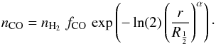 (A.2)The dust opacity is the number density of dust particles times the cross-section (πa2Qe) and is
 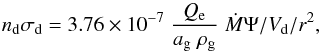 (A.3)where in the present paper the dust velocity (Vd) is taken equal to the gas velocity (V). The dust optical depth that is used in Eq. (6) is the integral over radius of this quantity,
  (A.4)Less important parameters are the inner radius of the shell where the calculation starts (a few stellar radii), and the outer radius which is arbitrarily set to 15 . Finally, the CO excitation temperature profile needs to be provided.
The quantities nH2, nCO and ndσd are calculated on a radial grid spaced logarithmically between the inner and outer radius. For θ = 0 (see the structure of the envelope in Fig. A.1) the column density can be determined exactly and compared to the numerical integration. A grid with 200 radial points ensures that the column densities are accurate to 0.1% even for the largest mass-loss rates.
For each point in the grid k(ri,θ) (see Eq. (6)) is determined which requires the calculation of the column densities and optical depth along the lines of sights (los) for all angles θ. The procedure in Appendix A in Li et al. (2014) is followed, which outlines how the case of angles 0 <θ<π/ 2 (e.g. the los  ) can be calculated, and how the case of π/ 2 <θ<π (e.g. the los
  ) can be recast into a problem with θ = π/ 2 (the los
  ) and the los
  .
.
The integral over θ is split into two parts. From zero to the angle (π − β), where β is the angle where the los grazes the central star (or the adopted inner radius of the envelope), i.e.  , and the angle from (π − β) to π, which covers the angle subtended by the central object.
The shielding function ΘH2,CO is interpolated for the calculated CO and H2 column densities and average temperature. The dependence of the shielding on the excitation temperature is small, so that assuming a typical temperature is allowed. The value Θdust follows from exp ( − τdust).
The shielding functions were compared for different angular grid sizes and in the end a grid of 130 uniformly distributed points in θ between 0 and (π − β) was adopted.
In this way the photodissociation rate at the radial grid points is determined. However, the integration of Eq. (2) to determine the CO profile requires care as the spatial scale for the change in abundance can change by orders of magnitude throughout the envelope. The spatial scale for a significant change in abundance at distance r is (V/I(r)). By performing some numerical tests the following procedure was adopted. If (fV/I(r)) (with f = 0.003) is smaller than the distance between consecutive grid points, then the integral in Eq. (2) is evaluated with the photodissociation rate that was previously calculated. If not, (fV/I(r)) is used as stepsize and the photodissociation rate at ri = ri − 1 + (fV/I(ri − 1)) is determined. The integration is continued until x(ri) = 0.001.
With the profile x(r) calculated, values for and α are determined by fitting a straight line to ln( − (ln(x(r)) / ln(2))) versus ln(r) over the range 0.29 <x(r) < 0.89.
Figure A.2 illustrates the effect of the shielding. It obviously depends on the parameters of the model (shown is the standard model) and on the location in the envelope (shown is  for that model) but the shape is typical. The least shielding is in the forward radial direction. Shielding increases as the angle θ increases (Fig. A.1), in this case by a factor of ~2 up to θ ~ 90°. Radiation penetrating from the far side of the envelope is greatly reduced.
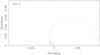 |
Fig. A.2 Total shielding k(r,θ) as a function of angle near |
All Tables
All Figures
|
Fig. 1 Solid lines indicates the CO photodissociation rate as a function of radial distance for the standard model. The dashed line indicates the value of |
| In the text | |
|
Fig. 2 Solid line indicates the relative CO profile for the standard model, while the dashed line gives the profile for the fitted values of |
| In the text | |
|
Fig. 3 CO abundance profiles for MLRs between 10-11 and 10-4M⊙ yr-1 in steps of a decade. |
| In the text | |
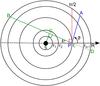 |
Fig. A.1 Structure of the circumstellar envelope model of an AGB star (adopted from Li et al. 2014). |
| In the text | |
|
Fig. A.2 Total shielding k(r,θ) as a function of angle near |
| In the text | |
Current usage metrics show cumulative count of Article Views (full-text article views including HTML views, PDF and ePub downloads, according to the available data) and Abstracts Views on Vision4Press platform.
Data correspond to usage on the plateform after 2015. The current usage metrics is available 48-96 hours after online publication and is updated daily on week days.
Initial download of the metrics may take a while.