| Issue |
A&A
Volume 606, October 2017
|
|
|---|---|---|
| Article Number | A101 | |
| Number of page(s) | 4 | |
| Section | Catalogs and data | |
| DOI | https://doi.org/10.1051/0004-6361/201731632 | |
| Published online | 20 October 2017 | |
Optical linear polarization measurements of quasars obtained with the 3.6 m telescope at the La Silla Observatory⋆,⋆⋆
1 Institut d’Astrophysique et de Géophysique, Université de Liège, Allée du 6 Août 19c, B5c, 4000 Liège, Belgium
e-mail: This email address is being protected from spambots. You need JavaScript enabled to view it.
2 Department of Physics and Astronomy, York University, Toronto, Ontario M3J 1P3, Canada
Received: 24 July 2017
Accepted: 29 August 2017
Abstract
We report 192 previously unpublished optical linear polarization measurements of quasars obtained in April 2003, April 2007, and October 2007 with the European Southern Observatory Faint Object Spectrograph and Camera (EFOSC2) instrument attached to the 3.6 m telescope at the La Silla Observatory. Each quasar was observed once. Among the 192 quasars, 89 have a polarization degree p ≥ 0.6%, 18 have p ≥ 2%, and two have p ≥ 10%.
Key words: quasars: general / polarization
Based on observations made with the ESO 3.6 m Telescope at the La Silla Observatory under program ID 071.B-0460, 079.A-0625, 080.A-0017.
Full Table 4 is only available at the CDS via anonymous ftp to cdsarc.u-strasbg.fr (130.79.128.5) or via http://cdsarc.u-strasbg.fr/viz-bin/qcat?J/A+A/606/A101
Senior Research Associate F.R.S.-FNRS.
© ESO, 2017
1. Introduction
The linear polarization of optical light is an important feature in the study of quasars and other active galactic nuclei (AGN). Usually attributed to scattering, polarization is directly related to the object symmetry axis, and is at the heart of AGN unification models.
In the present paper, we report new optical linear polarization measurements of quasars obtained with EFOSC2, the European Southern Observatory (ESO) Faint Object Spectrograph and Camera instrument attached to the 3.6 m telescope at the La Silla Observatory. Although the observations were designed for various scientific goals, the quality of the data is homogeneous. In Sect. 2 we describe the observing procedure. Data reduction and measurements are summarized in Sect. 3. The table with the final measurements is outlined in Sect. 4.
2. Observations
The polarimetric observations were carried out in April 2003, April 2007, and October 2007 at the European Southern Observatory, La Silla, using the 3.6 m telescope equipped with EFOSC2 attached to the Cassegrain focus. Linear polarimetry is performed by inserting a Wollaston prism into the parallel beam, which splits the incoming light rays into two orthogonally polarized beams. Each object in the field has therefore two orthogonally polarized images on the charge-coupled device (CCD) detector, separated by 20″. To avoid image overlapping, one puts at the telescope focal plane a special mask made of alternating transparent and opaque parallel strips whose widths correspond to the splitting. The final CCD image then consists of alternate orthogonally polarized strips of the sky, two of them containing the polarized images of the object itself (di Serego Alighieri 1989, 1997; Lamy & Hutsemékers 1999). Since the two orthogonally polarized images of the object are simultaneously recorded, the polarization measurements do not depend on variable atmospheric transparency, or seeing. In order to derive the normalized Stokes parameters q and u, four frames are obtained with the half-wave plate (HWP) at four different position angles (0°, 22.5°, 45°, and 67.5°). While only two different orientations of the HWP are sufficient to measure the linear polarization, the two additional orientations allow us to remove most of the instrumental polarization (di Serego Alighieri 1989). Polarized and unpolarized standard stars were observed to unambiguously fix the zero-point of the polarization position angle, to estimate the instrumental polarization, and to check the whole observing and reduction process.
Most targets are quasars with redshifts between one and three, and V magnitudes between 17 and 19. They were mostly selected from amongst broad absorption line (BAL), radio-loud, or red quasars that are more likely to be significantly polarized. All observations but one were obtained through the Bessel V filter (ESO# 641), the Bessel R filter (ESO# 642), and the Gunn i filter (ESO# 705), with typical exposure times per frame ranging between one and ten minutes. One faint target was observed unfiltered (in “white light”). The CCD#40 mounted on EFOSC2 is a 2k × 2k CCD with a pixel size of 15 μm corresponding to 0.158′′ on the sky in the 1 × 1 binning mode.
3. Data reduction and measurements
Observed standard stars.
Residual polarization from field stars.
Polarization of distant stars.
Polarization of quasars.
The q and u Stokes parameters are computed from the measurement of the integrated intensity ratios between the upper and lower orthogonally polarized images of the object, for the four different orientations of the half-wave plate. They are calculated with respect to the instrumental reference frame according to 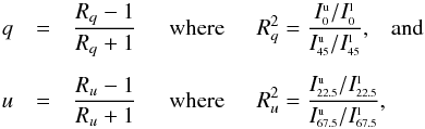 (1)where Iu and Il refer to the intensities (electron counts) integrated over the upper and lower images of the object, respectively. The photometric measurements were done using the procedures described in Lamy & Hutsemékers (1999) and Sluse et al. (2005). The positions of the upper and lower images are measured at subpixel precision by fitting two-dimensional Gaussian profiles. The intensities are then integrated in circles centered on the upper and lower images, and the Stokes parameters are computed for various values of the aperture radius. Since the Stokes parameters are found to be stable against radius changes, we adopt a fixed aperture radius of 3.0 × [(2ln2)− 1/2 HWHM] , where HWHM represents the mean half-width at half-maximum of the two-dimensional Gaussian profile. In a few cases, the Stokes parameters strongly fluctuate when changing the aperture radius, making their measurement unreliable. The combination of measurements using four frames obtained with different HWP orientations removes most of the instrumental polarization, and corrects the effects of image distortions introduced by the HWP (di Serego Alighieri 1989; Lamy & Hutsemékers 1999). The uncertainties σq and σu are evaluated by computing the errors on the intensities Iu and Il from the read-out noise and the photon noise in the object and the sky background, and then by propagating these errors. Typical uncertainties are around 0.2% for either q or u.
A zero-point angle offset correction, filter dependent, is then applied to the quasar normalized Stokes parameters q and u in order to convert the polarization angle measured in the instrumental reference frame to the equatorial reference direction. This angle offset is determined using polarized standard stars observed every night in each filter (Table 1). For all stars observed during a given run and within a given filter, the values of the offset agree within 1°. The polarization of unpolarized standard stars (Table 1) is typically around 0.10 ± 0.05% for all runs indicating that the instrumental polarization is small and essentially removed by the observing procedure.
Since on most frames field stars are simultaneously recorded, one can use them to estimate the residual instrumental polarization and/or interstellar polarization. While a frame-by-frame correction of the quasar Stokes parameters is in principle possible, it is hazardous since we are never sure that the polarization of field stars correctly represents the interstellar polarization that could affect distant quasars. Moreover, the field stars can be fainter than the quasar so that a frame-by-frame correction would introduce uncertainties on the quasar polarization larger than the residual polarization itself. We then compute the weighted average ( and
and  ) and dispersion (
 ) of the normalized Stokes parameters of field stars, considering the n⋆ frames with suitable field stars obtained during a given run. These values are given in Table 2. Frames centered on quasars and distant stars (Table 3) are considered. We usually measure a single field star per frame; in some cases this star is made up of the combination of two to three fainter stars observed on the same frame. Only stellar polarizations with uncertainties σq and σu better than 0.3% are used in the average. The small values and dispersions of the average Stokes parameters reported in Table 2 confirm the low level of uncorrected instrumental polarization.
In order to minimize systematic errors in the sample, we conservatively take this residual instrumental and/or averaged interstellar polarization into account by subtracting the systematic and from the measured q and u, and by adding quadratically to their errors. Then, from the corrected q and u values, the polarization degree is evaluated using p = (q2 + u2)1/2 and the associated error using σp ≃ σq ≃ σu. In addition, p must be corrected for the statistical bias inherent to the fact that p is always a positive quantity. The debiased value p0 of the polarization degree is obtained by using the Wardle & Kronberg (1974) estimator, which was found to be a reasonably good estimator of the true polarization degree (Simmons & Stewart 1985). The polarization position angle θ is obtained by solving the equations q = pcos2θ and u = psin2θ. The uncertainty of the polarization position angle θ is estimated from the standard Serkowski (1962) formula, where the debiased value p0 is conservatively used instead of p, that is,  (see also Wardle & Kronberg 1974). Due to the HWP chromatism over broad-band filters, an additional error ≤2–3° on θ should be accounted for (cf. the wavelength dependence of the polarization position angle offset in di Serego Alighieri 1997).
These procedures, the values of the residual polarization, and the distribution of field star polarization are similar to those reported in Sluse et al. (2005). We refer to that paper for more details and an exhaustive discussion of the effect of the various corrections. As a conclusion, the polarization of field stars is most often ≤0.3% so that virtually every quasar with a polarization degree higher than 0.6% is intrinsically polarized, in agreement with previous studies (Berriman et al. 1990; Lamy & Hutsemékers 2000).
Since the distance of field stars in unknown, we have measured the V-band polarization of a few very distant stars (d> 10 kpc) to further check the amount of interstellar polarization in the direction of our targets. These measurements are reported in Table 3. All these stars appear to have low polarization. Although the sample is small, this confirms that, on average, contamination by interstellar polarization should be unimportant for quasars at high galactic latitudes (| bII | > 30°) and with polarization degrees higher than 0.6%.
4. Polarization data
The full Table 4, available at the Strasbourg astronomical data center (CDS), summarizes the polarization measurements obtained for 192 different quasars (72 in April 2003, 28 in April 2007, and 92 in October 2007). Unreliable measurements were discarded. Eighty-nine quasars have p ≥ 0.6%, 18 have p ≥ 2%, and two have p ≥ 10%. Column (1) gives the quasar name from the NASA/IPAC extragalactic database (NED), Cols. (2) and (3) the equatorial coordinates (J2000), Col. (4) the redshift z, Col. (5) the filter used (V, R, i, and W for no filter), and Col. (6) the date of observation (year-month-day). Columns (7) and (8) give the normalized Stokes parameters q and u in percent corrected for the systematic residual polarization given in Table 2. The normalized Stokes parameters are given in the equatorial reference frame. Columns (9) and (10) give the polarization degree p and its error σp in percent. Column (11) gives the debiased polarization degree p0 in percent. Columns (12) and (13) give the polarization position angle θ east-of-north and its error σθ, in degrees. When p<σp, the polarization angle is undefined and its value put to 999. Finally “C?” in Col. (14) indicate quasars with p> 0.6% and for which the polarization of the field stars is comparable or higher, that is objects whose polarization has possibly been contaminated by interstellar polarization.
Among the eight objects with p ≥ 3% reported in Table 4, three of them were already known for their high linear polarization: [HB89] 0219-164 (Mead et al. 1990), WISE J125908.45-231038.6 (Sluse et al. 2005), and [HB89] 2155-152 (Wardle et al. 1984). Moreover, the linear polarization of WISE J125908.45-231038.6 and [HB89] 2155-152, uncorrected for the systematic polarization given in Table 2, has been discussed in Hutsemékers et al. (2010) together with circular polarization measurements. Among the five remaining objects with first-time polarization measurements, two are BAL quasars: SDSS J145603.07+011445.4 (Hall et al. 2002) and SDSS J232550.73-002200.3 (Trump et al. 2006). [HB89] 1243-072, WISE J131250.90-042449.9 and PKS 2140-43 are Parkes radio sources, the first two also belonging to the Fermi Gamma-ray Space Telescope source catalog (Nolan et al. 2012).
Acknowledgments
This research has made use of the NASA/IPAC Extragalactic Database (NED), which is operated by the Jet Propulsion Laboratory, California Institute of Technology, under contract with the National Aeronautics and Space Administration.
References
- Beers, T. C., Chiba, M., Yoshii, Y., et al. 2000, AJ, 119, 2866 [NASA ADS] [CrossRef] [Google Scholar]
- Berriman, G., Schmidt, G. D., West, S. C., & Stockman, H. S. 1990, ApJS, 74, 869 [NASA ADS] [CrossRef] [Google Scholar]
- Clewley, L., Warren, S. J., Hewett, P. C., Norris, J. E., & Evans, N. W. 2004, MNRAS, 352, 285 [NASA ADS] [CrossRef] [Google Scholar]
- di Serego Alighieri, S. 1989, in ESO Conf. and Workshop Proc., ESO/ST-ECF Data Analysis Workshop, eds. P. J. Grosbøl, F. Murtagh, & R. H. Warmels, 31, 157 [Google Scholar]
- di Serego Alighieri, S. 1997, in Polarimetry with large telescopes, eds. J. M. Rodríguez Espinosa, A. Herrero, & F. Sánchez, 287 [Google Scholar]
- Fossati, L., Bagnulo, S., Mason, E., & Landi Degl’Innocenti, E. 2007, in The Future of Photometric, Spectrophotometric and Polarimetric Standardization, ed. C. Sterken, ASP Conf. Ser., 364, 503 [Google Scholar]
- Hall, P. B., Anderson, S. F., Strauss, M. A., et al. 2002, ApJS, 141, 267 [NASA ADS] [CrossRef] [Google Scholar]
- Hutsemékers, D., Borguet, B., Sluse, D., Cabanac, R., & Lamy, H. 2010, A&A, 520, L7 [NASA ADS] [CrossRef] [EDP Sciences] [Google Scholar]
- Lamy, H., & Hutsemékers, D. 1999, The Messenger, 96, 25 [NASA ADS] [Google Scholar]
- Lamy, H., & Hutsemékers, D. 2000, A&AS, 142, 451 [NASA ADS] [CrossRef] [EDP Sciences] [Google Scholar]
- Mead, A. R. G., Ballard, K. R., Brand, P. W. J. L., et al. 1990, A&AS, 83, 183 [Google Scholar]
- Nolan, P. L., Abdo, A. A., Ackermann, M., et al. 2012, ApJS, 199, 31 [NASA ADS] [CrossRef] [Google Scholar]
- Serkowski, K. 1962, Adv. Astron. Astrophys., 1, 289 [NASA ADS] [CrossRef] [Google Scholar]
- Simmons, J. F. L., & Stewart, B. G. 1985, A&A, 142, 100 [NASA ADS] [Google Scholar]
- Sluse, D., Hutsemékers, D., Lamy, H., Cabanac, R., & Quintana, H. 2005, A&A, 433, 757 [NASA ADS] [CrossRef] [EDP Sciences] [Google Scholar]
- Trump, J. R., Hall, P. B., Reichard, T. A., et al. 2006, ApJS, 165, 1 [NASA ADS] [CrossRef] [Google Scholar]
- Turnshek, D. A., Bohlin, R. C., Williamson, II, R. L., et al. 1990, AJ, 99, 1243 [NASA ADS] [CrossRef] [Google Scholar]
- Wardle, J. F. C., & Kronberg, P. P. 1974, ApJ, 194, 249 [NASA ADS] [CrossRef] [Google Scholar]
- Wardle, J. F. C., Moore, R. L., & Angel, J. R. P. 1984, ApJ, 279, 93 [NASA ADS] [CrossRef] [Google Scholar]
All Tables
Current usage metrics show cumulative count of Article Views (full-text article views including HTML views, PDF and ePub downloads, according to the available data) and Abstracts Views on Vision4Press platform.
Data correspond to usage on the plateform after 2015. The current usage metrics is available 48-96 hours after online publication and is updated daily on week days.
Initial download of the metrics may take a while.