Strong constraints on hadronic models of blazar activity from Fermi and IceCube stacking analysis

Andrii Neronov; Dmitri V. Semikoz; Ksenia Ptitsyna

doi:10.1051/0004-6361/201630098

Free Access

Issue		A&A Volume 603, July 2017


Article Number		A135
Number of page(s)		8
Section		Extragalactic astronomy
DOI		https://doi.org/10.1051/0004-6361/201630098
Published online		20 July 2017

A&A 603, A135 (2017)

Strong constraints on hadronic models of blazar activity from Fermi and IceCube stacking analysis

Andrii Neronov¹, Dmitri V. Semikoz²^,3 and Ksenia Ptitsyna⁴

¹ Astronomy Department, University of Geneva, Ch. d’Ecogia 16, 1290 Versoix, Switzerland
e-mail: andrii.neronov@unige.ch
² APC, Universite Paris Diderot, CNRS/IN2P3, CEA/IRFU, Observatoire de Paris, Sorbonne Paris Cité, 119, 75205 Paris, France
³ National Research Nuclear University MEPHI (Moscow Engineering Physics Institute), Kashirskoe highway 31, 115409 Moscow, Russia
⁴ Institute for Nuclear Research of the Russian Academy of Sciences, 60th October Anniversary Prospect 7a, 117312 Moscow, Russia

Received: 19 November 2016
Accepted: 4 June 2017

Abstract

Context. High-energy emission from blazars is produced by electrons that are either accelerated directly, under the assumption of leptonic models of blazar activity, or produced in interactions of accelerated protons with matter and radiation fields, under the assumption of hadronic models. The hadronic models predict that γ-ray emission is accompanied by neutrino emission with comparable total energy.

Aims. We derive constraints on the hadronic models of activity of blazars imposed by non-detection of neutrino flux from a population of γ-ray emitting blazars.

Methods. We stacked the γ-ray and muon neutrino flux from 749 blazars situated in the declination strip above − 5°.

Results. Non-detection of neutrino flux from the stacked blazar sample rules out the proton-induced cascade models in which the high-energy emission is powered by interactions of a shock-accelerated proton beam in the active galactic nucleus (AGN) jet with the ambient matter or radiation field of the black hole accretion disk. The result also remains valid for the case of interactions in the scattered radiation field in the broad line region. The IceCube constraint could be avoided if the spectrum of accelerated protons is sharply peaking in the ultra-high-energy cosmic ray range, as in the models of acceleration in the magnetic reconnection regions or in the vacuum gaps of black hole magnetospheres. Models based on these acceleration mechanisms are only consistent with the data if characteristic energies of accelerated protons are higher than 10¹⁹ eV. The constraint could also be avoided if the hadronic emission component of γ-ray flux is largely sub-dominant compared to the leptonic component and/or if it only appears during flaring activity episodes, which provide negligible contribution to the time-averaged source flux.

Key words: galaxies: active / gamma rays: galaxies / neutrinos

© ESO, 2017

1. Introduction

Supermassive black holes in some 10% of active galactic nuclei (AGNs) accelerate particles and produce jets that could be occasionally aligned along the line of sight (Urry & Padovani 1995). In this case the AGN appears as a blazar that is detectable in the γ-ray band. The details of the mechanisms of jet generation and particle acceleration in AGN are not clear. High-energy electrons producing the observed synchrotron and inverse Compton emission can either be accelerated directly, as in leptonic models of AGN activity, or can be generated in interactions of high-energy protons and nuclei, as in hadronic models.

Different types of hadronic models correspond to different possible mechanisms of acceleration and interactions of high-energy protons and nuclei. The proton-induced cascade model(s) ascribe the γ-ray emission to the inverse Compton emission from electromagnetic cascade initiated by the interactions of high-energy protons during their propagation through the radiation field of the AGN central engine and jet (Mannheim & Biermann 1989, 1992; Mannheim 1993). Otherwise, the γ-ray component of the spectrum could be dominated by the synchrotron radiation from the highest energy protons, as suggested in the proton synchrotron models (Mücke & Protheroe 2001; Aharonian 2002; Mücke et al. 2003).

The proton induced cascade (PIC) models are subdivided onto two sub-types, depending on the nature of interactions of the high-energy protons. In one case, the cascade can be initiated by interactions of high-energy protons with dense radiation field created by the AGN accretion disk or the jet (Mannheim & Biermann 1989, 1992; Begelman et al. 1990; Mannheim 1993; Halzen & Zas 1997; Neronov & Semikoz 2002; Kalashev et al. 2015). Otherwise, the cascade can be initiated by interactions of protons with low-energy protons from the ambient medium, for example from the accretion flow or from the interstellar environment of the black hole (Eichler 1979; Neronov et al. 2008; Neronov & Ribordy 2009a).

The details of cascade development depend on the spectrum of primary protons. The most common assumption is that the acceleration site is a relativistic shock in the AGN jet. In this case, the proton spectrum is expected to be a cut-off power-law dN_p/ dE ∝ E^{− Γ}exp⁽−E/E_cut⁾ with the slope Γ ≃ 2 and cut-off energy E_cut, which could reach the ultra-high-energy cosmic ray (UHECR) energy range. This statement is somewhat uncertain because of the uncertainty of the efficiency of geometry of magnetic field geometry in the AGN jet shocks, such as turbulence properties and orientation of the ordered field component with respect to the shock normal (Bednarz & Ostrowski 1998; Lemoine et al. 2006; Pelletier et al. 2009). An alternative possibility for particle acceleration is acceleration in magnetic reconnection regions or events in the AGN accretion flow (Lesch & Birk 1997; Romanova & Lovelace 1992) or in the jet, and acceleration in the vacuum gaps in the black hole magnetosphere (Beskin et al. 1992; Hirotani & Okamoto 1998; Levinson 2000; Neronov et al. 2005, 2009; Neronov & Aharonian 2007; Aleksić et al. 2014; Hirotani & Pu 2016; Broderick & Tchekhovskoy 2015; Ptitsyna & Neronov 2016). Contrary to the shock acceleration, these types of acceleration mechanisms produce high-energy particle spectra sharply peaked at a characteristic energy so that the effective Γ is Γ ≪ 2.

A straightforward difference between leptonic and hadronic models of blazar activity is the absence or presence of neutrino emission accompanying the γ-ray emission. No significant neutrino flux is expected in the leptonic models. To the contrary, the specific of hadronic cascades is that the overall neutrino energy flux is always comparable (at least within an order of magnitude) with the electromagnetic flux from the source.

IceCube neutrino telescope has discovered an astrophysical neutrino signal in the energy range in which AGN and, in particular, blazars are expected to produce neutrino flux (Aartsen et al. 2013, 2014b, 2015b,a,c; IceCube Collaboration 2013; IceCube Collaboration et al. 2016b). Search for neutrino signal from individual blazars or blazar samples did not provide positive detections up to now (Tchernin et al. 2013; IceCube Collaboration et al. 2016a). Also the stacking analysis did not provide solid evidence for neutrino flux from blazars (Aartsen et al. 2014a; Glüsenkamp 2016; Padovani et al. 2016). The absence of multiplet events in the IceCube muon neutrino data gives additional constraints on the density of neutrino sources, which also constrain blazars as possible neutrino sources (Murase & Waxman 2016). However, time coincidence of a neutrino arrival with a blazar outburst was claimed to support the hypothesis of the blazar origin of the astrophysical neutrino signal (Kadler et al. 2016).

Non-detection of the signal from the γ-ray brightest blazars was used by Tchernin et al. (2013) to derive limits on the parameters of the PIC hadronic models of blazars. The data of IC-40 detector limit E_cut and Γ to be roughly (1)In what follows we combine the updated IceCube neutrino data (IceCube Collaboration et al. 2016b) with the data of Fermi γ-ray telescope to improve previously derived bounds on Γ and E_cut. We use stacking, rather than individual source analysis, and consider cumulative γ-ray and neutrino spectra of a large number of northern sky blazars.

Our results severely limit the class of PIC models consistent with the combined γ-ray and neutrino data. Most of the hadronic component-dominated models of time-averaged flux from blazars, based on the assumption of shock acceleration of protons interacting either with low-energy protons or with the UV radiation field, appear to be ruled out. Models that avoid the γ-ray + neutrino constraint are those predicting the accelerated particle spectra sharply peaked in the UHECR range. However, in these models the parameters of particle acceleration mechanisms also have to be tuned to provide the highest possible efficiencies. The limits imposed by the IceCube data could be avoided in the “mixed” hadronic plus leptonic models of blazar emission. For such models, our analysis severely limits the fraction of electromagnetic power that could come from hadronic interactions. The hadronic and leptonic components could be also “mixed in time”; for instance the hadronic emission might be responsible for flaring activity, while leptonic emission dominates the steady-state flux. Such models are also not directly constrained by our analysis. The contribution of such sources to IceCube flux is subdominant.

2. Stacking analysis approach to γ-ray and neutrino spectra

Within the PIC models, the overall energy flux of neutrinos and photons from the source is comparable, at least within an order of magnitude, i.e. (2)The neutrino signal from individual blazars is detectable in background-free regime in the energy band above several hundred TeV (IceCube Collaboration et al. 2016b). Suppose that the upper limit on neutrino flux from an individual source is F_ν,lim. Non-detection of neutrinos from any of N stacked sources provides an upper limit on “typical” neutrino flux from a source, i.e. (3)The upper limits on the flux of individual sources in the Northern Hemisphere reported by IceCube (IceCube Collaboration et al. 2016a) range between F_ν,lim ≃ 10^-9 GeV/(cm² s) and 3 × 10^-9 GeV/(cm² s), for the declinations ranging from 0 to 90 degrees. The best sensitivity is achieved in the energy range around 100 TeV, where the atmospheric neutrino background becomes low enough so that the signal with the flux level F_ν,lim is detectable in nearly background free regime. The limiting flux level for individual sources is comparable to the typical flux level of of blazars detected by Fermi-LAT telescope. Thus, source-by-source analysis could only mildly constrain the limits of the PIC type models by imposing a requirement that the bulk of the neutrino flux is not emitted in the 100 TeV band. This limits the properties of the parent proton spectrum, as reported by Tchernin et al. (2013).

A size of the population of GeV γ-ray detected blazars is ~10³. Although the flux of most of the Fermi-LAT detected blazars is typically one or two orders of magnitude lower than the fluxes of the brightest blazars, the cumulative γ-ray flux of all the detected blazars is still an order of magnitude larger than that of an individual bright blazar. Thus, the expected cumulative neutrino signal from the population of the γ-ray detected blazars is a factor of 10 larger than the flux from any individual bright blazar. If the typical energies of neutrinos from blazars are much higher than 100 TeV, as suggested by the IceCube constraints derived from the analysis of individual bright blazars (Tchernin et al. 2013), the signal from individual blazars is not detectable, but an order of magnitude stronger cumulative neutrino signal from γ-ray loud blazar population might still be detectable at the highest energies.

3. Data analysis

3.1. Fermi-LAT

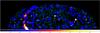	Fig. 1 IceCube muon neutrino events (white ellipses) with direction uncertainty less than 4 degrees, overlaid over Fermi-LAT countmap pf the northern sky in the energy range above 1 TeV, smoothed with 3 degree Gaussian. Green crosses show blazars selected for the stacking analysis.
Open with DEXTER

For our stacking analysis we consider publicly available data of Fermi-LAT telescope collected during the time period between August 2008 and June 2016. We filter the LAT event list with the help of gtselect – gtmktime tools following the recommendations of the Fermi-LAT team¹ to select only events belonging to the CLEAN sub-class. For each selected source we extract the spectrum using the aperture photometry method estimating the exposure with the help of gtexposure tool. We sum the source counts, the background counts and the exposures in the direction of all the selected sources to produce a cumulative source spectrum. For each source, the source signal is extracted from a circle of the radius 1° around the source position. The background is estimated from a 1° circle displaced by 2° from the source position.

The list of blazars selected for the stacking analysis includes N = 749 flat spectrum radio quasars (FSRQ) and BL Lacerta (BL Lac) type objects at declinations Dec > −5° listed in the third Fermi-LAT source catalogue (Acero et al. 2015). This choice of the declination range is determined by sky region from which the IceCube astrophysical neutrino signal is collected (IceCube Collaboration et al. 2016b).

Figure 2 shows the resulting cumulative spectrum of blazars in this part of the sky. One could see that it is nearly identical to the cumulative spectrum of high Galactic latitude sources found in the Ackermann et al. (2015). This is not surprising, given the fact that blazars constitute the dominant extragalactic source population.

3.2. IceCube

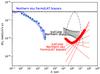Fig. 2

Cumulative γ-ray (blue data points) spectrum and neutrino flux upper limit (red) for the Northern Hemisphere blazars. The blue shaded band shows the spectrum of extragalactic sources resolved by Fermi telescope from Ackermann et al. (2015). The black hatched bow-tie shows the IceCube astrophysical neutrino flux in the muon neutrino channel from IceCube Collaboration et al. (2016b). The grey dashed line shows a model neutrino spectrum for a PIC model from Tchernin et al. (2013).

Open with DEXTER

We use the list of 29 muon neutrino events with energy proxies above 200 TeV reported by IceCube Collaboration et al. (2016b). Three out of the 29 events have large statistical uncertainty of direction reconstruction (larger than 3°). The chance coincidence probability for such events to have one of the 749 blazars within their error ellipse is of the order of one. We remove these events from the analysis. Rejection of these events reduces the effective exposure of IceCube data set by 3/29 ≃ 10%.

The 90% error ellipses of the 26 neutrino events retained for the analysis do not contain γ-ray detected blazars, except for one blazar, OP 313, which is at the border of the error ellipse of the muon neutrino event 36. This is consistent with a chance coincidence expectation. The event number 36 has the energy proxy E = 200 TeV and only 0.45 “signalness” value (IceCube Collaboration et al. 2016b), i.e. is more likely to be part of the atmospheric neutrino background. A 90% upper limit on the number of muon neutrino events with energy proxies above 200 TeV from blazars is, assuming the Poisson statistics of the signal, (4)The spectrum of neutrino emission from blazars is, in general, unknown. To derive an upper limit on the neutrino flux from blazars for arbitrary spectral shape, for different slopes Γ we calculate the maximal possible normalisation κ of a power-law neutrino flux (5)where E_∗ is normalisation energy fixed here to E_∗ = 1 PeV. We scan over the slopes Γ to find an “envelope” curve of the different maximal possible flux power laws, as described by Tchernin et al. (2013). Realistic neutrino emission spectra can typically be well approximated by power laws in the energy range where the IceCube sensitivity is highest (about PeV for the considered IceCube data set), unless the spectrum has a high- or low-energy cut-off exactly in the IceCube sensitivity range. This implies that envelope curve of the upper limits on the power-law type spectra can be also used for the realistic spectra; the spectra consistent with the data can at most “touch” the envelope curve from below.

To derive the envelope curve, the IceCube exposure for ν_μ (or ) in the energy range above 400 TeV is well approximated by a power law (6)with the normalisation TA_∗ ≃ (7/2) × 10¹⁴ cm² s, averaged over the solid angle Ω = 2π(1−cos(95°)) and counting only muon neutrinos, at a reference energy E_∗ = 1 PeV and the slope p = 0.34 (IceCube Collaboration et al. 2016b).

The expected number of muon neutrinos and anti-neutrinos in an energy range E_min<E_ν<E_max for a given flux normalisation κ is (7)where the factor 1/3 accounts for the fact that the muon neutrinos constitute 1/3 of the signal (adopting standard assumptions about production mechanism and mixing).

Muons produced in the charged current interactions outside the IceCube detector have initial energies E_μ ≃ (1−y_cc)E_ν, where y_cc is the average inelasticity of the charged current interactions (Gandhi et al. 1996). The energies of most detected neutrino-induced muons are much lower than the initial muon energy because of the energy loss in the rock dE_μ/ dx = −(a + bE_μ) (Chirkin & Rhode 2004), so that the distribution of final energies of muons originating from monoenergetic neutrinos with energy E_ν steadily undergoing charged current interactions all over a large distance through the rock/ice is dN_μ/ dE ∝ E^-1 in the energy range E<E₀, down to the energy E_crit = a/b ≃ 1 TeV. This suggests the probability density function for the muon energy (Neronov & Ribordy 2009b) (8)The distribution of the energies of the muon events is then (9)Integrating the muon distribution in the energy range (E_min,E_max) one finds (10)which differs from the neutrino number by a factor (ln(E_μ/E_crit))^-1 ≃ 0.2.

Normalising N_μ = N_lim one finds κ for different values of Γ. The result is shown by the red straight lines in Fig. 2. The red thick curve shows the envelope of all maximal allowed power laws. In Γ < p + 1 ≃ 1.3, the signal statistics is dominated by the highest energy events and the maximal normalisation of the power law depends on the high-energy cut-off in the spectrum. We have fixed E_max to 10¹⁸ eV in our calculation.

4. Results and discussion

4.1. Inconsistency of the data with proton induced cascade model with shock-accelerated protons in the jet

One could see from Fig. 2 that the upper limit on the neutrino flux from blazars in the PeV energy range is two orders of magnitude below the expected flux level. The mismatch between the γ-ray flux level and neutrino flux upper limits rule our hadronic models in which neutrino spectra are expected to produce most of the power in the PeV energy range.

The pion production in pγ interactions occurs only above an energy threshold (11)where ϵ is the characteristic energy of photons from the radiative environment of the AGN. The energies of neutrinos originating from the charged pion decays are typically below ≲10% of the parent proton energy, (12)Pion decays transfer nearly equal power to the neutrino and electromagnetic emission. Development of electromagnetic cascade in the source transfers the electromagnetic power to the GeV-TeV energy band. The horizontal dashed line in Fig. 2 shows an estimate of the electromagnetic power from the blazar population. Contrary to the electromagnetic power, the neutrino emission power stays in the energy band (12).

This is the case for the proton-induced cascade models in which the shock-accelerated protons interact with the radiation field of accretion disk. Conventional geometrically thin and optically thick accretion disks in AGN have temperatures reaching 10⁴ K in the innermost portions of the disk close to the last stable orbit (Shakura & Sunyaev 1976; Frank et al. 1992). Protons accelerated near the black hole or in the innermost portion of the AGN jet interact with the direct UV radiation from the disk or with the disk radiation scattered in the broad line region. This inevitably produces neutrinos with energies in the PeV range. An example of neutrino spectrum calculated for proton spectrum with Γ = 2 and E_cut = 10¹⁷ eV interacting with the soft photons from the accretion disk with the spectrum peaking at ϵ = 15 eV (from Tchernin et al. 2013) is shown by the grey dashed line in Fig. 2. A realistic neutrino spectrum produced by an entire population of blazars might be more complicated than this model because both Γ and E_cut are distributed in a certain range. Still a model with fixed E_cut and Γ could serve as a “reference” model for the entire population, where the reference parameter values are the distribution averages. This makes sense if the parameter distributions are concentrated around certain values, for example Γ is always close to 2 in the models of shock acceleration.

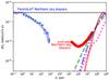	Fig. 3 Comparison of the IceCube upper limit on the neutrino flux with predictions of PIC models of blazars.
Open with DEXTER

The IceCube bound could be avoided if the bulk of neutrino power is emitted in an energy band different from 0.1–10 PeV. This is the case if the soft photon targets for pγ interactions are in the infrared or microwave range. This type of interaction is considered in the model of Essey et al. (2010, 2011). The characteristic energy of the cosmic microwave background photons is ϵ ≃ 10^-3 eV. The magenta dotted line in Fig. 3 shows a representative model of neutrino spectrum from interactions of protons with the spectrum E^-2 with high-energy cut-off at 10²⁰ eV during their propagation through the CMB and extragalactic background light radiation fields (Essey et al. 2011). Normalising the model flux on the average γ-ray flux from blazars, one finds that the model spectrum is consistent with the IceCube constraint.

Other types of hadronic models that are severely constrained by combined IceCube and Fermi data are those in which shock accelerated protons interact with the ambient medium protons and nuclei. In this case the pion production threshold is in the 100 MeV range and the neutrino spectrum in the energy range above the threshold approximately repeats the proton spectrum. If the proton spectrum is a power law with a slope close to 2, the neutrino spectrum in the PeV energy range is also a power law with a slope close to 2 and with the energy flux comparable to that of the γ-ray flux within a factor of two. The mismatch between the maximal possible normalisation of an E^-2 type neutrino spectrum and the dashed horizontal line in Figs. 2 and 3 is two orders of magnitude, which means that the model is ruled out. Consistency of the model with the data can only be restored if the acceleration process typically produces proton spectrum with a slope that is softer than 2.4. In this case the spectra of γ-rays and neutrinos originating from pion decays are also soft power laws and the neutrino flux in the PeV range are within the IceCube upper limit. This type of hadronic model is, however, constrained via source-by-source analysis, as reported for example by Tchernin et al. (2013).

Blazars are highly variable sources exhibiting periods of activity intermittent with the quiescence periods. Differences in the chains of production reactions of the PeV neutrinos and GeV photons could, in principle, lead to significant differences in the timing properties of the γ-ray and neutrino signals. In particular, higher energy neutrinos that are produced at the very beginning of development of the PIC might come before the lower energy photons emitted at the end of the cascade development. This mismatch between the timing properties of neutrino and γ-ray signals hampers the search of the neutrino emission from blazars through a search of the neutrino counterparts of the γ-ray signal and the γ-ray counterparts of the neutrino signal on a source-by-source basis. However, it does not affect the results of the time-averaged stacking analysis presented above because the timescale of the analysis (eight years of Fermi data and six years of IceCube data) is much longer than the timescale of the γ-ray flares (minutes-to-months). All the neutrino signals associated with the γ-ray flares of individual blazars should be contained within the multi-year exposure with the possible exception of flares that occurred at the very beginning of the exposure time.

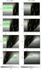Fig. 4

Energies of protons accelerated in magnetospheric vacuum gaps near a black hole of mass M = 5 × 10⁹M_⊙ (left column) or 5 × 10⁸M_⊙ (right column) surrounded by RIAF with synchrotron emission spectrum peaking in the infrared at ϵ = 0.1 eV (top row) to 10^-4 eV (bottom row). Red dashed lines show the dimensionless gap height h. Green solid curves show proton energies. Dark grey parts of the diagram show the parameter range excluded by the IceCube plus Fermi data set. Green shaded areas correspond to the allowed range of parameters.

Open with DEXTER

4.2. Constraints on models with sharply peaked proton spectra

The combined IceCube and Fermi constraint on the proton-induced cascade model can be avoided if the high-energy protons are not produced by the shock acceleration process. If the protons are injected by acceleration taking place in large-scale electric fields as is the case for the field in magnetic reconnection regions or in vacuum gaps in the black hole magnetosphere, the spectrum of protons is sharply peaked at a particular energy rather than having a power-law shape. If the characteristic energy of the acceleration process is large enough, the peak energy of the neutrino spectrum is determined by the characteristic proton energy, rather than by the threshold of the pγ reaction. The blue dash-dotted line in Fig. 3 shows the neutrino spectrum from interactions of protons with energies 3 × 10¹⁹ GeV interacting with ϵ = 10 eV photons. The low-energy part of the model spectrum is tangent to the envelope of the IceCube upper limits. This means that the models of PIC in the AGN accretion disk radiation fields are consistent with the limits if the proton spectrum has a sharp low-energy cut-off, (13)An alternative possibility for avoiding the IceCube plus Fermi constraint is to consider models in which the accretion on the black hole forms a radiatively inefficient accretion flow (RIAF). These types of models are believed to be applicable to low luminosity radio galaxies and BL Lac type objects. In this case the low-energy radiation from the accretion flow is synchrotron radiation from electrons heated to relativistic temperatures by collisions with protons. Synchrotron radiation from a RIAF peaks in the infrared range according to Narayan et al. (1998)ϵ ≲ 0.1 eV, and the neutrino spectrum peaks in the energy range above 10¹⁷ eV. This is illustrated by the red solid curve in Fig. 3, which is the neutrino spectrum produced in interactions of 10¹⁹ eV protons with 0.1 eV photons. The model spectrum is consistent with the IceCube data, so that models with proton spectrum with low-energy cut-off at (14)are also consistent with the data.

The combined IceCube and Fermi constraint can be also avoided in the PIC model, in which high-energy protons interact with low-energy protons from the accretion flow if the high-energy proton spectrum is sharply peaked at high energies. The green dashed line in Fig. 3 shows the calculation of the model neutrino spectrum from interactions of protons with energy 2 × 10²⁰ eV with the low-energy protons. One could see that the low-energy part of the neutrino spectrum is tangent to the IceCube upper bound envelope curve. This means that models based on pp interactions are constrained to produce extremely high-energy protons, (15)

4.3. Proton energies in black hole magnetospheric gap models

Energies of protons accelerated in the gap of the height H in the magnetosphere of a black hole of the mass M are limited by the finite extent of the gap, which is defined by the onset of electron-positron pair production on the soft photon background field present in the magnetosphere. The gap height depends on the luminosity L and size R of the soft photon field, the characteristic soft photon energy ϵ, and the rate of electron/proton acceleration in the gap, which is determined by the specific angular momentum of the black hole a (Beskin et al. 1992; Hirotani & Okamoto 1998; Levinson 2000; Neronov et al. 2005, 2009; Neronov & Aharonian 2007; Aleksić et al. 2014; Hirotani & Pu 2016; Broderick & Tchekhovskoy 2015; Ptitsyna & Neronov 2016).

Figure 4 shows the attainable proton energy as a function of source luminosity L and magnetic field B, calculated within the framework discussed by Ptitsyna & Neronov (2016). The assumption of the model is that the black hole accretes in the RIAF mode in which the soft photon field is produced via synchrotron emission from electrons heated to the temperatures 10–100 MeV by the protons. The RIAF synchrotron radiation spectrum typically peaks in the infrared range as opposed to the UV-dominated spectrum of an optically thick, geometrically thin accretion disk. The two columns of the figure correspond to two different black hole masses. The four rows correspond to various soft photon fields in the AGN central engine. In all the cases the infrared/microwave soft photon source is supposed to be distributed over a region of the size 10R_Schw, where R_Schw is the Schwarzschild radius of the black hole.

The process of the pair production starts to limit the gap height when the luminosity reaches certain (magnetic field dependent) value around 10⁴⁰ erg/s. At lower luminosities of the RIAF the density of the soft photon field is not sufficient for the pair production within the extent of the black hole magnetosphere on the distance scale R ~ R_Schw about the Schwarzschild radius of the black hole. In this case the limiting proton energy is estimated as (16)where M is the black hole mass. The limit E_p> 6 × 10¹⁸ eV converts into a lower bound on magnetic field strength in the innermost part of the RIAF (17)Proton energies also drop below 6 × 10¹⁸ eV at high values of B. In this case the proton synchrotron loss limits the energies of protons, as in the models of Mücke & Protheroe (2001), Aharonian (2002), Mücke et al. (2003). This type of model is not directly constrained by a combination of the Fermi-LAT and IceCube data discussed above.

The pair production initiated by electrons accelerated in the gap also gets suppressed at high luminosities because the strong inverse Compton loss rate does not allow electrons to accelerate to the energies needed for the pair production. Suppression of the pair production at low and high luminosities allows acceleration of protons to the energies in excess of 10¹⁹ eV. However, in this case protons start to produce pairs themselves when accelerated to energies higher than the pair production threshold. This also limits the proton energies in the case of high luminosity RIAF as is clear from Fig. 4.

The green shaded regions in the various panels of Fig. 4 show the ranges of L,B parameter space in which proton energies reach >6 × 10¹⁸ GeV. Acceleration in the magnetospheric vacuum gaps near black holes surrounded by RIAF with such parameters would produce neutrino and electromagnetic emission consistent with IceCube and Fermi-LAT data. The IceCube plus Fermi-LAT constraints could be satisfied in only a very limited range of parameter space.

5. Conclusions

We have shown that a combination of IceCube and Fermi-LAT data rules out certain types of hadronic models of emission from blazars. The models that are inconsistent with the data are those in which the observed γ-ray emission is produced by a particle cascade initiated by shock accelerated protons in the UV radiation field of the AGN central engine. This result is consistent with analysis of Aartsen et al. (2017), which appeared after this paper was completed. Our analysis confirms the main result of that paper, i.e. that the astrophysical neutrino flux is generated by sources different from the GeV γ-ray loud blazars (BL Lacs and flat spectrum radio quasars).

Hadronic models of steady-state blazar emission consistent with the data are those in which high-energy protons spectra are sharply peaked in the UHECR range. An example of this type of model is that of proton acceleration in the vacuum gaps of black hole magnetospheres. We have shown that the IceCube and Fermi-LAT data constrain the parameter space of such models (luminosity and magnetic field in the RIAF surrounding the black hole). Models that are consistent with the data predict a neutrino flux originating from UHECR production in the blazars. This suggests that the model is testable via observations of neutrino flux in the energy range higher than that accessible with IceCube, E_ν ~ 0.1−1 EeV. An increase of IceCube exposure or an exploration of this energy range with dedicated detectors optimised for the 0.1–1 EeV range, such as CHANT (Neronov et al. 2017) or ARA (Ara Collaboration et al. 2012) could be used to test the model.

Our analysis also does not rule out the possibility of hadronic flares of blazars. It is still possible that the steady-state emission that dominates the time-averaged flux is determined by leptonic processes, while episodes of proton acceleration followed by PIC are responsible for the flaring activity. Such a possibility could be constrained via the search of neutrino counterparts of the γ-ray flares (or γ-ray counterparts of neutrino emission episodes of individual sources, but not with the time-averaged/stacking analysis. In any case, the hadronic flare contribution to the IceCube time-averaged flux should be small.

http://fermi.gsfc.nasa.gov/ssc/data/analysis/

Acknowledgments

We would like to thank S. Shoenen for useful discussions on details of IceCube results. The work of K.P. is supported by the Russian Science Foundation grant 14-12-01340.

References

Aartsen, M. G., Abbasi, R., Abdou, Y., et al. 2013, Phys. Rev. Lett., 111, 021103 [NASA ADS] [CrossRef] [PubMed] [Google Scholar]
Aartsen, M. G., Ackermann, M., Adams, J., et al. 2014a, ApJ, 796, 109 [NASA ADS] [CrossRef] [Google Scholar]
Aartsen, M. G., Ackermann, M., Adams, J., et al. 2014b, Phys. Rev. Lett., 113, 101101 [NASA ADS] [CrossRef] [PubMed] [Google Scholar]
Aartsen, M. G., Abraham, K., Ackermann, M., et al. 2015a, ApJ, 809, 98 [NASA ADS] [CrossRef] [Google Scholar]
Aartsen, M. G., Abraham, K., Ackermann, M., et al. 2015b, Phys. Rev. D, 91, 022001 [NASA ADS] [CrossRef] [Google Scholar]
Aartsen, M. G., Abraham, K., Ackermann, M., et al. 2015c, Phys. Rev. Lett., 115, 081102 [NASA ADS] [CrossRef] [PubMed] [Google Scholar]
Aartsen, M. G., Abraham, K., Ackermann, M., et al. 2017, ApJ, 835, 45 [NASA ADS] [CrossRef] [Google Scholar]
Acero, F., Ackermann, M., Ajello, M., et al. 2015, ApJS, 218, 23 [NASA ADS] [CrossRef] [Google Scholar]
Ackermann, M., Ajello, M., Albert, A., et al. 2015, ApJ, 799, 86 [NASA ADS] [CrossRef] [Google Scholar]
Aharonian, F. A. 2002, MNRAS, 332, 215 [NASA ADS] [CrossRef] [Google Scholar]
Aleksić, J., Ansoldi, S., Antonelli, L. A., et al. 2014, Science, 346, 1080 [NASA ADS] [CrossRef] [Google Scholar]
Ara Collaboration, Allison, P., Auffenberg, J., et al. 2012, Astropart. Phys., 35, 457 [NASA ADS] [CrossRef] [Google Scholar]
Bednarz, J., & Ostrowski, M. 1998, Phys. Rev. Lett., 80, 3911 [NASA ADS] [CrossRef] [Google Scholar]
Begelman, M. C., Rudak, B., & Sikora, M. 1990, ApJ, 362, 38 [NASA ADS] [CrossRef] [Google Scholar]
Beskin, V. S., Istomin, Y. N., & Parev, V. I. 1992, Sov. Astron., 36, 642 [NASA ADS] [Google Scholar]
Broderick, A. E., & Tchekhovskoy, A. 2015, ApJ, 809, 97 [NASA ADS] [CrossRef] [Google Scholar]
Chirkin, D., & Rhode, W. 2004, High Energy Physics – Phenomenology [arXiv:hep-ph/0407075] [Google Scholar]
Eichler, D. 1979, ApJ, 232, 106 [NASA ADS] [CrossRef] [Google Scholar]
Essey, W., Kalashev, O. E., Kusenko, A., & Beacom, J. F. 2010, Phys. Rev. Lett., 104, 141102 [NASA ADS] [CrossRef] [Google Scholar]
Essey, W., Kalashev, O., Kusenko, A., & Beacom, J. F. 2011, ApJ, 731, 51 [NASA ADS] [CrossRef] [Google Scholar]
Frank, J., King, A., & Raine, D. 1992, Accretion power in astrophysics [Google Scholar]
Gandhi, R., Quigg, C., Hall Reno, M., & Sarcevic, I. 1996, Astropart. Phys., 5, 81 [NASA ADS] [CrossRef] [Google Scholar]
Glüsenkamp, T. 2016, in EPJ Web Conf., 121, 05006 [Google Scholar]
Halzen, F., & Zas, E. 1997, ApJ, 488, 669 [NASA ADS] [CrossRef] [Google Scholar]
Hirotani, K., & Okamoto, I. 1998, ApJ, 497, 563 [NASA ADS] [CrossRef] [Google Scholar]
Hirotani, K., & Pu, H.-Y. 2016, ApJ, 818, 50 [NASA ADS] [CrossRef] [Google Scholar]
IceCube Collaboration 2013, Science, 342, 1242856 [CrossRef] [PubMed] [Google Scholar]
IceCube Collaboration, Aartsen, M. G., Abraham, K., et al. 2016a, ApJ, 835, 151 [NASA ADS] [CrossRef] [Google Scholar]
IceCube Collaboration, Aartsen, M. G., Abraham, K., et al. 2016b, ApJ, 833, 3 [NASA ADS] [CrossRef] [Google Scholar]
Kadler, M., Krauß, F., Mannheim, K., et al. 2016, Nat. Phys., 12, 807 [NASA ADS] [CrossRef] [Google Scholar]
Kalashev, O., Semikoz, D., & Tkachev, I. 2015, J. Exp. Theor. Phys., 120, 541 [NASA ADS] [CrossRef] [Google Scholar]
Lemoine, M., Pelletier, G., & Revenu, B. 2006, ApJ, 645, L129 [NASA ADS] [CrossRef] [Google Scholar]
Lesch, H., & Birk, G. T. 1997, A&A, 324, 461 [NASA ADS] [Google Scholar]
Levinson, A. 2000, Phys. Rev. Lett., 85, 912 [NASA ADS] [CrossRef] [PubMed] [Google Scholar]
Mannheim, K. 1993, A&A, 269, 67 [NASA ADS] [Google Scholar]
Mannheim, K., & Biermann, P. L. 1989, A&A, 221, 211 [NASA ADS] [Google Scholar]
Mannheim, K., & Biermann, P. L. 1992, A&A, 253, L21 [NASA ADS] [Google Scholar]
Mücke, A., & Protheroe, R. J. 2001, Astropart. Phys., 15, 121 [NASA ADS] [CrossRef] [Google Scholar]
Mücke, A., Protheroe, R. J., Engel, R., Rachen, J. P., & Stanev, T. 2003, Astropart. Phys., 18, 593 [NASA ADS] [CrossRef] [Google Scholar]
Murase, K., & Waxman, E. 2016, Phys. Rev. D, 94, 103006 [NASA ADS] [CrossRef] [Google Scholar]
Narayan, R., Mahadevan, R., & Quataert, E. 1998, in Theory of Black Hole Accretion Disks, eds. M. A. Abramowicz, G. Björnsson, & J. E. Pringle, 148 [Google Scholar]
Neronov, A., & Aharonian, F. A. 2007, ApJ, 671, 85 [NASA ADS] [CrossRef] [Google Scholar]
Neronov, A., & Ribordy, M. 2009a, Phys. Rev. D, 80, 083008 [NASA ADS] [CrossRef] [Google Scholar]
Neronov, A., & Ribordy, M. 2009b, Phys. Rev. D, 79, 043013 [NASA ADS] [CrossRef] [Google Scholar]
Neronov, A. Y., & Semikoz, D. V. 2002, Phys. Rev. D, 66, 123003 [NASA ADS] [CrossRef] [Google Scholar]
Neronov, A., Tinyakov, P., & Tkachev, I. 2005, Sov. J. Exp. Theor. Phys., 100, 656 [NASA ADS] [CrossRef] [Google Scholar]
Neronov, A., Semikoz, D., & Sibiryakov, S. 2008, MNRAS, 391, 949 [NASA ADS] [CrossRef] [Google Scholar]
Neronov, A. Y., Semikoz, D. V., & Tkachev, I. I. 2009, New J. Phys., 11, 065015 [NASA ADS] [CrossRef] [Google Scholar]
Neronov, A., Semikoz, D. V., Anchordoqui, L. A., Adams, J. H., & Olinto, A. V. 2017, Phys. Rev. D, 95, 023004 [NASA ADS] [CrossRef] [Google Scholar]
Padovani, P., Resconi, E., Giommi, P., Arsioli, B., & Chang, Y. L. 2016, MNRAS, 457, 3582 [NASA ADS] [CrossRef] [Google Scholar]
Pelletier, G., Lemoine, M., & Marcowith, A. 2009, MNRAS, 393, 587 [NASA ADS] [CrossRef] [Google Scholar]
Ptitsyna, K., & Neronov, A. 2016, A&A, 593, A8 [NASA ADS] [CrossRef] [EDP Sciences] [Google Scholar]
Romanova, M. M., & Lovelace, R. V. E. 1992, A&A, 262, 26 [NASA ADS] [Google Scholar]
Shakura, N. I., & Sunyaev, R. A. 1976, MNRAS, 175, 613 [NASA ADS] [CrossRef] [Google Scholar]
Tchernin, C., Aguilar, J. A., Neronov, A., & Montaruli, T. 2013, A&A, 555, A70 [NASA ADS] [CrossRef] [EDP Sciences] [Google Scholar]
Urry, C. M., & Padovani, P. 1995, PASP, 107, 803 [NASA ADS] [CrossRef] [Google Scholar]

All Figures

	Fig. 1 IceCube muon neutrino events (white ellipses) with direction uncertainty less than 4 degrees, overlaid over Fermi-LAT countmap pf the northern sky in the energy range above 1 TeV, smoothed with 3 degree Gaussian. Green crosses show blazars selected for the stacking analysis.
Open with DEXTER
In the text

	Fig. 2 Cumulative γ-ray (blue data points) spectrum and neutrino flux upper limit (red) for the Northern Hemisphere blazars. The blue shaded band shows the spectrum of extragalactic sources resolved by Fermi telescope from Ackermann et al. (2015). The black hatched bow-tie shows the IceCube astrophysical neutrino flux in the muon neutrino channel from IceCube Collaboration et al. (2016b). The grey dashed line shows a model neutrino spectrum for a PIC model from Tchernin et al. (2013).
Open with DEXTER
In the text

	Fig. 3 Comparison of the IceCube upper limit on the neutrino flux with predictions of PIC models of blazars.
Open with DEXTER
In the text

	Fig. 4 Energies of protons accelerated in magnetospheric vacuum gaps near a black hole of mass M = 5 × 10⁹M_⊙ (left column) or 5 × 10⁸M_⊙ (right column) surrounded by RIAF with synchrotron emission spectrum peaking in the infrared at ϵ = 0.1 eV (top row) to 10^-4 eV (bottom row). Red dashed lines show the dimensionless gap height h. Green solid curves show proton energies. Dark grey parts of the diagram show the parameter range excluded by the IceCube plus Fermi data set. Green shaded areas correspond to the allowed range of parameters.
Open with DEXTER
In the text

Current usage metrics show cumulative count of Article Views (full-text article views including HTML views, PDF and ePub downloads, according to the available data) and Abstracts Views on Vision4Press platform.

Data correspond to usage on the plateform after 2015. The current usage metrics is available 48-96 hours after online publication and is updated daily on week days.

Initial download of the metrics may take a while.