© ESO, 2017

1. Introduction

Most of the non-thermal emission seen in powerful astrophysical objects such as supernovae remnants (SNR), pulsar wind nebulae, and gamma-ray bursts is believed to arise through the synchrotron and inverse Compton radiation of electrons accelerated at a strong collisionless shock front (e.g. Blandford & Eichler 1987; Bykov et al. 2012).

It has been long recognized that the acceleration of particles is intimately related to the self-generation of turbulence or to the amplification of pre-existing magnetic fluctuations in the shock precursor. This precursor delimits the region of space upstream of the shock where the particles that are accelerated at the shock front interact with the background plasma. In this context, the observation of radiative signatures from this precursor would bring new and unprecedented information on the turbulence, on the acceleration process and the shock physics, which is currently probed indirectly through the radiation of the shocked plasma on much greater space and time scales. Among the top questions to be addressed are the following: what is the magnetization of the background flow? What is the level of turbulence and on what scales is it distributed? How are the accelerated particles transported in the self-generated/amplified turbulence?

The precursor is bounded by the length over which the accelerated particles return to the shock front after scattering in the ambient magnetized flow. The hierarchy between the typical scale of this precursor (ℓ_p) and that of the shocked downstream region (ℓ_d ~ R, R radius of the shock) – namely ℓ_p ≪ ℓ_d – is precisely what makes the detection of the precursor difficult. Its synchrotron contribution has been debated in the literature. For instance, Sironi & Spitkovsky (2009) observe in their numerical simulation of a relativistic shock front a net signal from the shock precursor, at higher energies than the radiation from the downstream flow, while Gedalin et al. (2008) have argued that the strong enhancement of the turbulence in the transition layer of a relativistic collisionless shock should leave a distinct imprint in the synchrotron spectrum. In sub-relativistic shock waves, rather broad shock transitions seen in X-ray have been interpreted as the signature of an extended synchrotron precursor, although this broadening might otherwise represent deviations of the shock front away from sphericity (Vink 2013). Numerical simulations of such X-ray images, including a contribution from the synchrotron precursor indicate that the possibility of detection is directly related to the unknown length scale of the precursor, and the feasibility of a detection remains uncertain (see e.g. Achterberg et al. 1994; Ammosov et al. 1994; Reynolds 1998; Berezhko et al. 2003; Long et al. 2003; Ellison & Cassam-Chenaï 2005; Morlino et al. 2010).

The main objectives of this paper are to characterize the synchrotron signature of the precursor and to assert the feasibility of a detection, in both relativistic and non-relativistic sources. We also discuss the degree of polarization, since it may prove an essential tool in extracting the precursor signal. In the relativistic regime, a Lorentz aberration generically implies a configuration in which the source is not spatially resolved and where the flow and the line of sight are nearly coincident. Consequently, the synchrotron contribution must be extracted from the overall spectral energy distribution. As we show in Sect. 2, the precursor spectrum is generally much harder than that of the shocked region, suggesting that a detection, if feasible, should occur at the highest frequencies, typically in the X-ray range.

In the non-relativistic regime, the shock front can be seen edge-on, which offers the possibility of direct imaging of the precursor. We calculate this spectro-morphological contribution in detail in Sect. 3; in particular, we argue that the detection of linear polarization on small angular scales upstream of the shock would provide a net signature of this precursor. We summarize our results and provide conclusions in Sect. 4.

2. Precursor of relativistic shock fronts

We consider a relativistic source, with the observer on-axis, as is the case of a gamma-ray burst afterglow. On both analytical and numerical grounds, little is known about the structure of the precursor on the space and time scales that are representative of astrophysical objects. We thus consider a general picture, in which both the precursor and the shocked downstream plasma are populated by a background magnetic field and by a magnetized turbulence. The fraction of local total energy density stored in magnetic turbulence is written ϵ_Bd downstream and ϵ_Bp in the precursor, while σ represents the magnetization of the background flow. Consequently, the comoving downstream magnetic field reads $\mathit{\delta }{\mathit{B}}_{\mathrm{|}\mathrm{d}}\hspace{0.17em}\mathrm{=}\hspace{0.17em}{{}^{\mathrm{(}}\mathit{ϵ}_{\mathit{B}\mathrm{d}}\mathrm{8}\mathit{\pi }\hspace{0.17em}\mathrm{2}{\mathrm{\Gamma }}_{\mathrm{sh}}^{\mathrm{2}}\hspace{0.17em}{\mathit{n}}_{\mathrm{u}}{\mathit{m}}_{\mathrm{p}}{\mathit{c}}^{\mathrm{2}}{}^{\mathrm{)}}}^{\mathrm{1}\mathit{/}\mathrm{2}}$, while the precursor frame turbulent field reads $\mathit{\delta }{\mathit{B}}_{\mathrm{|}\mathrm{p}}\hspace{0.17em}\mathrm{=}\hspace{0.17em}{{}^{\mathrm{(}}\mathit{ϵ}_{\mathit{B}\mathrm{p}}\mathrm{8}\mathit{\pi }\hspace{0.17em}{\mathit{n}}_{\mathrm{u}}{\mathit{m}}_{\mathrm{p}}{\mathit{c}}^{\mathrm{2}}{}^{\mathrm{)}}}^{\mathrm{1}\mathit{/}\mathrm{2}}$ (see below for the association of the precursor frame with the upstream frame) and the background upstream frame field B_{| u} = ⁽σ8πn_um_pc^2)1/2; n_u denotes the proper density of the unshocked plasma and Γ_sh the bulk Lorentz factor of the shock front relative to the background plasma.

For simplicity, and to reduce the number of free parameters, we consider here a turbulence of homogeneous power both upstream and downstream. Both theory and phenomenology suggest that the downstream turbulence should decay away from the shock front through collisionless damping (see e.g. Chang et al. 2008; Lemoine 2013, 2015a,b; Lemoine et al. 2013). However, at late observing times, such as those considered here, the resulting synchrotron self-Compton spectrum can be approximated with an effective ϵ_Bd parameter of low value, representative in some way of the average fraction over the blast length scale (see Lemoine 2015b). Considering the distribution of magnetic energy in the shock precursor, we take into account its possible evolution with distance through the average value of ϵ_Bp and through two extreme models, which are discussed below.

An important issue in the calculation of the synchrotron emission and its polarization is the choice of reference frame. In the background magnetic field, the relevant frame for the synchrotron process is the upstream frame (neglecting any deceleration of the flow on the scale of the precursor). In weakly magnetized shock waves, the turbulence is believed to be self-generated through filamentation-type instabilities (e.g. Medvedev & Loeb 1999). For the particular case of the Weibel instability, there is a frame in which the turbulence is mostly magnetic in nature; it can be shown that this frame moves at sub-relativistic velocities with respect to the background plasma (Pelletier et al., in prep.). Up to this sub-relativistic motion the relevant frame is again the upstream frame, and in this frame the accelerated electron population is strongly beamed forward into an angle ~1/Γ_sh.

The accelerated population is modelled with a power law between a minimum Lorentz factor γ_{m | p} ~ 2Γ_shγ_m (γ_m being the corresponding shock frame quantity), a spectral index s, and a maximum Lorentz factor determined by energy losses. The minimum Lorentz factor of the accelerated population is defined as usual by (e.g. Piran 2004) γ_m ≃ | s−2 | / | s−1 | ϵ_eΓ_shm_p/m_e so that the accelerated particle population is described, in the shock frame, by $\frac{\mathrm{d}{\mathit{n}}_{\mathrm{e}\mathrm{|}\mathrm{sh}}}{\mathrm{d}{\mathit{\gamma }}_{\mathrm{e}}}\hspace{0.17em}\mathrm{=}\hspace{0.17em}\frac{{\mathit{ϵ}}_{\mathrm{e}}{\mathit{e}}_{\mathrm{sh}}}{{\mathit{\gamma }}_{\mathrm{m}}{\mathit{m}}_{\mathrm{e}}{\mathit{c}}^{\mathrm{2}}}\frac{\mathrm{|}\mathit{s}\mathrm{-}\mathrm{2}\mathrm{|}}{{\mathit{\gamma }}_{\mathrm{m}}}{\left(\frac{{\mathit{\gamma }}_{\mathrm{e}}}{{\mathit{\gamma }}_{\mathrm{m}}}\right)}^{\mathrm{-}\mathit{s}}\mathrm{·}$(1)This guarantees that the total energy density of the accelerated electron population is normalized to ϵ_ee_sh, with e_sh the total energy density at the shock, while the number density of electrons is normalized to ${\mathit{e}}_{\mathrm{sh}}\mathit{/}{}^{\mathrm{(}}\mathrm{\Gamma }_{\mathrm{sh}}{\mathit{m}}_{\mathrm{p}}{\mathit{c}}^{\mathrm{2}}{}^{\mathrm{)}}$, as expected from the shock crossing conditions.

The electron radiation in the micro-turbulence can be described by a synchrotron process because the deflection of the pitch angle by an angle $\mathit{\delta \vartheta }\hspace{0.17em}\mathrm{=}\hspace{0.17em}\mathit{e\delta B}{\mathit{\lambda }}_{\mathit{\delta B}}\mathit{/}{}^{\mathrm{(}}\mathit{\gamma }_{\mathrm{e}}{\mathit{m}}_{\mathrm{e}}{\mathit{c}}^{\mathrm{2}}{}^{\mathrm{)}}$ over a coherence length λ_δB is much larger than the angle 1 /γ_e that determines the opening angle of the emission cone of radiation, see e.g. Kelner et al. (2013). Indeed, ${\mathit{\gamma }}_{\mathrm{e}}\mathit{\delta \vartheta }\hspace{0.17em}\mathrm{~}\hspace{0.17em}\mathrm{80}{\mathit{ϵ}}_{\mathit{B}\mathrm{p}\mathit{,}\mathrm{-}\mathrm{5}}^{\mathrm{1}\mathit{/}\mathrm{2}}{\mathit{\lambda }}_{\mathit{\delta B,}\mathrm{1}}{\mathit{\gamma }}_{\mathrm{e}}\mathit{/}{\mathit{\gamma }}_{\mathrm{m}\mathrm{|}\mathrm{p}}$, with λ_δB,1 = 0.1λ_δBc/ω_pi the coherence length scale in units of tens of skin depth scales; unless otherwise noted, we use cgs units with Q_x ≡ Q/ 10^x for any quantity Q.

Owing to Lorentz beaming of the electron population, we only consider the radiation emitted by the particles contained within an angle Δθ = 1/Γ_sh away from the line of sight, as measured from the source position. The synchrotron spectral power per unit solid angle of the precursor can then be expressed as $\frac{\mathrm{d}\mathit{P}}{\mathrm{d}\mathit{\nu }\mathrm{d\Omega }}\hspace{0.17em}\mathrm{=}\hspace{0.17em}\mathrm{\int }\mathrm{d}\mathit{r}{\mathit{r}}^{\mathrm{2}}\hspace{0.17em}\mathrm{d}{\mathit{\gamma }}_{\mathrm{e}}\hspace{0.17em}\hspace{0.17em}\frac{\mathrm{d}{\mathit{n}}_{\mathrm{e}\mathrm{|}\mathrm{p}}}{\mathrm{d}{\mathit{\gamma }}_{\mathrm{e}}}\hspace{0.17em}{\mathit{p}}_{\mathit{\nu }}$(2)in terms of dn_{e | p}/ dγ_e the electron distribution function in the precursor frame, and p_ν the isotropic spectral power of one electron (Ginzburg & Syrovatskii 1965; Legg & Westfold 1968): ${\mathit{p}}_{\mathit{\nu }}\hspace{0.17em}\mathrm{=}\hspace{0.17em}\sqrt{\mathrm{3}}{\mathit{e}}^{\mathrm{3}}{\mathit{B}}_{\mathrm{\perp }}\mathit{/}\mathrm{\left(}{\mathit{m}}_{\mathrm{e}}{\mathit{c}}^{\mathrm{2}}\mathrm{\right)}\mathit{F}\mathrm{\left(}\mathit{z}\mathrm{\right)}$ with $\mathit{F}\mathrm{\left(}\mathit{z}\mathrm{\right)}\hspace{0.17em}\mathrm{\equiv }\hspace{0.17em}\mathit{z}{{}^{\mathrm{\int }}}_{\mathit{z}}^{\mathrm{+}\mathrm{\infty }}\mathrm{d}\mathit{\eta }\hspace{0.17em}{\mathit{K}}_{\mathrm{5}\mathit{/}\mathrm{3}}\mathrm{\left(}\mathit{\eta }\mathrm{\right)}$, and z ≡ ν/ν_c, ${\mathit{\nu }}_{\mathrm{c}}\hspace{0.17em}\mathrm{\equiv }\hspace{0.17em}\mathrm{3}\mathit{e}{\mathit{B}}_{\mathrm{\perp }}{\mathit{\gamma }}_{\mathrm{e}}^{\mathrm{2}}\mathit{/}\mathrm{\left(}\mathrm{4}\mathit{\pi }{\mathit{m}}_{\mathrm{e}}\mathit{c}\mathrm{\right)}$ the peak frequency of synchrotron emission for an electron of Lorentz factor γ_e.

Solid angles do not appear in Eq. (2) because their product cancels out to unity; this product involves the solid angle of the volume element of the precursor (ΔΩ ≃ πΔθ²), the probability that an electron inside the precursor radiates towards the observer (p_→ ≃ δΩ/ΔΩ) and $\mathrm{1}\mathit{/}\mathit{\delta }\mathrm{\Omega }\hspace{0.17em}\mathrm{\simeq }\hspace{0.17em}{\mathit{\gamma }}_{\mathrm{e}}^{\mathrm{2}}\mathit{/}\mathit{\pi }$, which is the inverse solid angle of the emission of one electron along its near ballistic trajectory.

The distribution function of the electrons inside the precursor can be formally determined through a Lorentz transform of the corresponding distribution function in the shock frame, and the latter can be obtained by solving a stationary transport equation with a loss term corresponding to the finite residence time spent in the precursor. Here, we approximate this distribution function in the precursor frame as follows: $\frac{\mathrm{d}{\mathit{n}}_{\mathrm{e}\mathrm{|}\mathrm{p}}}{\mathrm{d}{\mathit{\gamma }}_{\mathrm{e}}}\hspace{0.17em}\mathrm{\simeq }\hspace{0.17em}\frac{{\mathit{R}}^{\mathrm{2}}}{{\mathit{r}}^{\mathrm{2}}}\hspace{0.17em}\frac{\mathrm{|}\mathit{s}\mathrm{-}\mathrm{1}\mathrm{|}}{{\mathit{\gamma }}_{\mathrm{m}\mathrm{|}\mathrm{p}}}{\left(\frac{{\mathit{\gamma }}_{\mathrm{e}}}{{\mathit{\gamma }}_{\mathrm{m}\mathrm{|}\mathrm{p}}}\right)}^{\mathrm{-}\mathit{s}}\hspace{0.17em}\mathrm{2}{\mathrm{\Gamma }}_{\mathrm{sh}}^{\mathrm{2}}{\mathit{n}}_{\mathrm{u}}\hspace{0.17em}\mathrm{\Theta }\mathrm{\left[}{\mathit{r}}_{\mathrm{p}}\mathrm{\right(}{\mathit{\gamma }}_{\mathrm{e}}\mathrm{)}\mathrm{-}{\mathit{r}}^{\mathrm{]}}\mathit{.}$(3)The Heaviside function models the finite length scale up to which particles of a given Lorentz factor can travel. This precursor length scale is related to the (upstream frame) residence time t_res through ${\mathit{r}}_{\mathrm{p}}\hspace{0.17em}\mathrm{=}\hspace{0.17em}\mathit{R}\mathrm{+}\mathit{c}{\mathit{t}}_{\mathrm{res}}\left(\mathrm{1}\mathrm{-}{\mathit{\beta }}_{\mathrm{sh}}\right)\hspace{0.17em}\mathrm{\simeq }\hspace{0.17em}\mathit{R}\mathrm{+}\mathit{c}{\mathit{t}}_{\mathrm{res}}\mathit{/}\mathrm{\left(}\mathrm{2}{\mathrm{\Gamma }}_{\mathrm{sh}}^{\mathrm{2}}\mathrm{\right)}$. The residence time can be calculated as the time it takes to deflect the accelerated electron by an angle ~1/Γ_sh (Achterberg et al. 2001; Milosavljević & Nakar 2006; Pelletier et al. 2009). If the background magnetic field controls the transport of the accelerated electrons, this residence time is ${\mathit{t}}_{\mathrm{res}}^{\mathrm{\left(}\mathrm{1}\mathrm{\right)}}\hspace{0.17em}\mathrm{\simeq }\hspace{0.17em}{\mathrm{\Gamma }}_{\mathrm{sh}}^{-1}{\mathit{\gamma }}_{\mathrm{e}}{\mathit{m}}_{\mathrm{e}}\mathit{c}\mathit{/}\mathrm{\left(}\mathit{e}{\mathit{B}}_{\mathrm{u}}\mathrm{\right)}$. In contrast, if pitch angle scattering in a micro-turbulence of length scale λ_δB governs the return of particles to the shock, ${\mathit{t}}_{\mathrm{res}}^{\mathrm{\left(}\mathrm{2}\mathrm{\right)}}\hspace{0.17em}\mathrm{\simeq }\hspace{0.17em}{\mathrm{\Gamma }}_{\mathrm{sh}}^{-2}{\mathit{\gamma }}_{\mathrm{e}}^{\mathrm{2}}{\mathit{m}}_{\mathrm{e}}^{\mathrm{2}}{\mathit{c}}^{\mathrm{3}}\mathit{/}\mathrm{\left(}{\mathit{\lambda }}_{\mathit{\delta B}}{\mathit{e}}^{\mathrm{2}}\mathit{\delta }{\mathit{B}}_{\mathrm{p}}^{\mathrm{2}}\mathrm{\right)}$. Whether one or the other occurs depends on γ_e and the hierarchy between B_u and δB_p. As the scattering frequency in a micro-turbulence scales as ${\mathit{\gamma }}_{\mathrm{e}}^{-2}$, while the gyrofrequency scales with ${\mathit{\gamma }}_{\mathrm{e}}^{-1}$, we expect the background field to control the residence time at higher energies. In order to bracket this realistic scenario, we consider in the following the above two extremes: (1) where regular deflection in a background field dominates at all energies and (2) where stochastic deflection in a small scale micro-turbulence of uniform energy density dominates at all energies. Correspondingly, we write ${\mathit{r}}_{\mathrm{p}}\mathrm{\left(}{\mathit{\gamma }}_{\mathrm{e}}\mathrm{\right)}\mathrm{=}\mathit{R}\mathrm{+}{\mathrm{\Delta }}_{\mathit{i}}{\mathit{\gamma }}_{\mathrm{e}}^{\mathit{i}}$, with i = 1,2 for models (1) or (2); ${\mathrm{\Delta }}_{\mathit{i}}\mathrm{=}\mathit{c}{\mathit{t}}_{\mathrm{res}}^{\mathrm{\left(}\mathit{i}\mathrm{\right)}}\mathit{/}\mathrm{\left(}\mathrm{2}{\mathrm{\Gamma }}_{\mathrm{sh}}^{\mathrm{2}}\mathrm{\right)}$.

In principle, to perform an accurate calculation of the synchrotron spectrum, one would need to specify both the residence time and the scaling of the micro-turbulent field with distance away from the shock. In order to bracket the uncertainty associated with transport and the evolution of the magnetic energy in the precursor, we use both extreme models (1) and (2). At small frequencies, corresponding to particles of small Lorentz factor exploring the near precursor, the transport should be governed by the stochastic field so that the synchrotron flux should be adequately described by model (2). The high-frequency part, however, corresponds to high-energy particles spending most of their time in the far precursor, where presumably the background magnetic field dominates the transport and the radiation process. One should thus expect the high-frequency part of the synchrotron spectrum to be described by model (1). These two extreme models should thus bracket adequately the synchrotron spectrum of the precursor.

Because the synchrotron flux scales with residence time, and because particles of larger Lorentz factor spend a greater amount of time in the precursor, the spectral power is expected to be harder than the standard slow-cooling spectrum of a population trapped in the downstream. This spectral dependence indeed derives from the integration of Eq. (2), giving a spectral flux on the detector 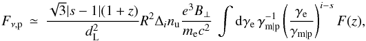${\mathit{F}}_{\mathit{\nu ,}\mathrm{p}}\hspace{0.17em}\mathrm{\simeq }\hspace{0.17em}\frac{\sqrt{\mathrm{3}}\mathrm{|}\mathit{s}\mathrm{-}\mathrm{1}\mathrm{|}\mathrm{(}\mathrm{1}\mathrm{+}\mathit{z}\mathrm{)}}{{\mathit{d}}_{\mathrm{L}}^{\mathrm{2}}}{\mathit{R}}^{\mathrm{2}}{\mathrm{\Delta }}_{\mathit{i}}{\mathit{n}}_{\mathrm{u}}\frac{{\mathit{e}}^{\mathrm{3}}{\mathit{B}}_{\mathrm{\perp }}}{{\mathit{m}}_{\mathrm{e}}{\mathit{c}}^{\mathrm{2}}}\hspace{0.17em}\mathrm{\int }\mathrm{d}{\mathit{\gamma }}_{\mathrm{e}}\hspace{0.17em}{\mathit{\gamma }}_{\mathrm{m}\mathrm{|}\mathrm{p}}^{-1}{\left(\frac{{\mathit{\gamma }}_{\mathrm{e}}}{{\mathit{\gamma }}_{\mathrm{m}\mathrm{|}\mathrm{p}}}\right)}^{\mathit{i}\mathrm{-}\mathit{s}}\mathit{F}\mathrm{\left(}\mathit{z}\mathrm{\right)}\mathit{,}$(4)which leads to a hard particle spectrum as integrated over the precursor length scale. Henceforth, all frequencies are written in the observer frame and Δ_i is evaluated at γ_{m | p}.

If i = 1, the last integral over γ can be performed using the standard results of Ginzburg & Syrovatskii (1965) and Legg & Westfold (1968), leading to a spectrum F_ν,p ∝ ν^(2−s)/2 in the inertial range – between the synchrotron peak frequencies ν_{m | p} and ${\mathit{\nu }}_{\max \mathrm{|}\mathrm{p}}^{\mathrm{\left(}\mathrm{1}\mathrm{\right)}}$ – of particles of respective Lorentz factor γ_{m | p} and γ_max; of course, F_ν,p ∝ ν^1/3 below ν_{m | p}. Hence, for s ≃ 2.3, νF_ν,p ∝ ν^0.85 up to the highest frequencies. If i = 2, these results are not applicable unless s> 7/3; if s< 7/3, the spectrum at any frequency ν is indeed dominated by the 1/3 low-frequency extension of the spectrum of particles radiating with a synchrotron peak frequency larger than ν. To calculate this contribution, the function F(z) can be approximated by its small z limit, F(z) ≃ 2^{− 1/3}3Γ(5/3) z^1/3 (z ≪ 1) and the integration can be performed over the effective distribution of particles in the precursor.

This results in a broken power-law approximation to the spectral flux of the precursor $\begin{array}{ccc}{\mathit{F}}_{\mathit{\nu ,}\mathrm{p}}& \hspace{0.17em}\mathrm{\simeq }\hspace{0.17em}& \frac{{\mathit{\varphi }}_{\mathit{i}}\mathrm{(}\mathrm{1}\mathrm{+}\mathit{z}\mathrm{)}}{{\mathit{d}}_{\mathrm{L}}^{\mathrm{2}}}{\mathit{R}}^{\mathrm{2}}\mathit{c}{\mathit{t}}_{\mathrm{res}}^{\mathrm{\left(}\mathit{i}\mathrm{\right)}}\mathrm{\left(}{\mathit{\gamma }}_{\mathrm{m}\mathrm{|}\mathrm{p}}\mathrm{\right)}\hspace{0.17em}{\mathit{n}}_{\mathrm{u}}\frac{{\mathit{e}}^{\mathrm{3}}{\mathit{B}}_{\mathrm{\perp }}}{{\mathit{m}}_{\mathrm{e}}{\mathit{c}}^{\mathrm{2}}}\hspace{0.17em}\hspace{0.17em}\mathrm{\Theta }\left[{\mathit{\nu }}_{\max \mathrm{|}\mathrm{p}}^{\mathrm{\left(}\mathit{i}\mathrm{\right)}}\mathrm{-}\mathit{\nu }\right]\hspace{0.17em}\\ & & \end{array}$(5)where, as before, i = 1, 2 and $\begin{array}{ccc}{\mathit{\varphi }}_{\mathrm{1}}& \hspace{0.17em}\mathrm{=}\hspace{0.17em}& \frac{\mathrm{|}\mathit{s}\mathrm{-}\mathrm{1}\mathrm{|}\sqrt{\mathrm{3}}}{\mathrm{4}}{\mathrm{2}}^{\mathrm{(}\mathit{s}\mathrm{-}\mathrm{2}\mathrm{)}\mathit{/}\mathrm{2}}\frac{\mathrm{4}\mathrm{+}\mathrm{3}\mathit{s}}{\mathrm{3}\mathit{s}}\mathrm{\Gamma }\left[\frac{\mathrm{3}\mathit{s}\mathrm{-}\mathrm{4}}{\mathrm{12}}\right]\mathrm{\Gamma }\left[\frac{\mathrm{3}\mathit{s}\mathrm{+}\mathrm{4}}{\mathrm{12}}\right]\\ {\mathit{a}}_{\mathrm{1}}& \hspace{0.17em}\mathrm{=}\hspace{0.17em}& \frac{\mathrm{2}\mathrm{-}\mathit{s}}{\mathrm{2}}\\ {\mathit{\varphi }}_{\mathrm{2}}& \hspace{0.17em}\mathrm{=}\hspace{0.17em}& \frac{\mathrm{3.7}\mathrm{|}\mathit{s}\mathrm{-}\mathrm{1}\mathrm{|}}{\mathrm{7}\mathit{/}\mathrm{3}\mathrm{-}\mathit{s}}\left[{\left(\frac{{\mathit{\gamma }}_{\max \mathrm{|}\mathrm{p}}}{{\mathit{\gamma }}_{\mathrm{m}\mathrm{|}\mathrm{p}}}\right)}^{\mathrm{7}\mathit{/}\mathrm{3}\mathrm{-}\mathit{s}}\mathrm{-}\mathrm{1}\right]\\ {\mathit{a}}_{\mathrm{2}}& \hspace{0.17em}\mathrm{=}\hspace{0.17em}& \end{array}$(6)The last two expressions assume s< 7/3. We note that the numerical prefactor ϕ₂ can become large if s comes close to 7/3, where the contributions of all particles add up to form the synchrotron spectrum at low frequencies. For s = 7/3, the factor $\mathrm{|}\mathit{s}\mathrm{-}\mathrm{7}\mathit{/}\mathrm{3}{\mathrm{|}}^{-1}\left[{{}^{\mathrm{(}}\mathit{\gamma }_{\max \mathrm{|}\mathrm{p}}\mathit{/}{\mathit{\gamma }}_{\mathrm{m}\mathrm{|}\mathrm{p}}{}^{\mathrm{)}}}^{\mathit{s}\mathrm{-}\mathrm{7}\mathit{/}\mathrm{3}}\mathrm{-}\mathrm{1}\right]\hspace{0.17em}\mathrm{\to }\hspace{0.17em}\ln {}^{\mathrm{(}}\mathit{\gamma }_{\max \mathrm{|}\mathrm{p}}\mathit{/}{\mathit{\gamma }}_{\mathrm{m}\mathrm{|}\mathrm{p}}{}^{\mathrm{)}}$.

It is possible to compare the precursor synchrotron flux to that produced downstream. Following Panaitescu & Kumar (2000), the latter can be expressed as ${\mathit{F}}_{\mathit{\nu ,}\mathrm{d}}\hspace{0.17em}\mathrm{\simeq }\hspace{0.17em}\mathrm{0.26}\mathrm{(}\mathrm{1}\mathrm{+}\mathit{z}\mathrm{)}\hspace{0.17em}{\mathit{d}}_{\mathrm{L}}^{-2}{\mathrm{\Gamma }}_{\mathrm{sh}}{\mathit{n}}_{\mathrm{u}}{\mathit{R}}^{\mathrm{3}}{\mathit{e}}^{\mathrm{3}}{\mathit{B}}_{\mathrm{d}}\mathit{/}\mathrm{\left(}{\mathit{m}}_{\mathrm{e}}{\mathit{c}}^{\mathrm{2}}\mathrm{\right)}{{}^{\mathrm{(}}\mathit{\nu }\mathit{/}{\mathit{\nu }}_{\mathrm{m}}{}^{\mathrm{)}}}^{\mathrm{(}\mathrm{1}\mathrm{-}\mathit{s}\mathrm{)}\mathit{/}\mathrm{2}}$ for ν>ν_m (assuming the slow-cooling regime and a homogeneous circumburst medium, ν_m representing the downstream minimum synchrotron frequency); B_d being a factor Γ_sh larger than B_u (both measured in their own comoving frames), 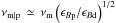${\mathit{\nu }}_{\mathrm{m}\mathrm{|}\mathrm{p}}\hspace{0.17em}\mathrm{\simeq }\hspace{0.17em}{\mathit{\nu }}_{\mathrm{m}}{{}^{\mathrm{(}}\mathit{ϵ}_{\mathit{B}\mathrm{p}}\mathit{/}{\mathit{ϵ}}_{\mathit{B}\mathrm{d}}{}^{\mathrm{)}}}^{\mathrm{1}\mathit{/}\mathrm{2}}$; consequently, the upstream contribution appears suppressed by a factor Δ_i/R at the minimum frequency (at equal ϵ_Bp and ϵ_Bd) up to the numerical prefactors, which can be traced back to the difference of volume occupied by the radiating electrons. At high frequencies, however, a larger relative contribution is expected from the precursor, due to the rising spectrum detailed above.

A detailed comparison thus requires a careful determination of the maximum Lorentz factor up to which particles can be accelerated, as well as an evaluation of the inverse Compton contribution from the downstream plasma, which takes over the synchrotron radiation at high frequencies.

The maximum Lorentz factor is determined by the competition between the residence time (both upstream and downstream) and the synchrotron or inverse Compton loss time. Given that the energy gain is of order unity per Fermi cycle, the acceleration time scale corresponds to the greater of the downstream or the upstream residence time (as evaluated in the same frame). Below, we instead calculate the maximum Lorentz factor associated with transport either downstream or upstream and keep the smaller of the two values. In a generic setting, inverse Compton losses dominate both downstream and upstream (Li & Waxman 2006).

We consider first the maximum energy for downstream particles, calculated in the downstream comoving frame. Assuming that particles scatter in a micro-turbulence of coherence length λ_δB, the maximum Lorentz factor for electrons corresponding to synchrotron and inverse Compton losses is ${\mathit{\gamma }}_{\max \mathrm{|}\mathrm{d}}\hspace{0.17em}\mathrm{\simeq }\hspace{0.17em}{\left[\frac{\mathrm{9}}{\mathrm{4}}\frac{{\mathit{\lambda }}_{\mathit{\delta B}}}{{\mathit{r}}_{\mathrm{e}}}\frac{\mathrm{1}}{\mathrm{1}\mathrm{+}\mathit{Y}}\right]}^{\mathrm{1}\mathit{/}\mathrm{3}}\mathit{,}$(7)where r_e ≃ 2.8 × 10^-13cm denotes the classical electron radius. A numerical estimate is ${\mathit{\gamma }}_{\mathrm{e}\mathit{,}\max \mathrm{|}\mathrm{d}}\hspace{0.17em}\mathrm{\simeq }\hspace{0.17em}{\mathrm{10}}^{\mathrm{7}}{{}^{\mathrm{(}}\mathrm{1}\mathrm{+}{\mathit{Y}}^{\mathrm{)}}}^{\mathrm{-}\mathrm{1}\mathit{/}\mathrm{3}}{\mathit{n}}_{\mathrm{0}}^{\mathrm{-}\mathrm{1}\mathit{/}\mathrm{6}}$. The Y Compton parameter is determined through (Sari & Esin 2001) $\mathit{Y}\hspace{0.17em}\mathrm{\simeq }\hspace{0.17em}{\left({\mathit{ϵ}}_{\mathrm{e}}\mathit{/}{\mathit{ϵ}}_{{\mathit{B}}_{\mathrm{d}}}\right)}^{\mathrm{1}\mathit{/}\mathrm{2}}{{}^{\mathrm{(}}\mathit{\gamma }_{\mathrm{c}\mathit{,}\mathrm{syn}}\mathit{/}{\mathit{\gamma }}_{\mathrm{m}}{}^{\mathrm{)}}}^{\mathrm{1}\mathrm{-}\mathit{s}\mathit{/}\mathrm{2}}$, with γ_c,syn the cooling Lorentz factor determined by synchrotron losses alone, i.e. the electron Lorentz factor (in the downstream frame) for which the synchrotron cooling length becomes comparable to the dynamical time scale t_dyn ≃ R/ (Γ_shc). We ignore Klein-Nishina suppression effects in the determination of γ_{e,max | d}; they may be important at very early observer times, leading to an effective , but become moderate at late times (Wang et al. 2010; Lemoine et al. 2013; Lemoine 2015b).

As discussed in various studies (see Pelletier et al. 2009; Bykov et al. 2012, and references therein) the above provides the correct way of defining the maximum Lorentz factor for acceleration. For reference, however, we also define a maximum Lorentz factor corresponding to the Bohm assumption, according to which the scattering frequency is given by the gyrofrequency: ${\mathit{\gamma }}_{\max \mathrm{|}\mathrm{d}}^{\mathrm{Bohm}}\hspace{0.17em}\mathrm{\simeq }\hspace{0.17em}{\left[\frac{\mathrm{6}\mathit{\pi e}}{{\mathit{\sigma }}_{\mathrm{T}}\mathit{\delta }{\mathit{B}}_{\mathrm{d}}\mathrm{(}\mathrm{1}\mathrm{+}{\mathit{Y}}^{\mathrm{)}}}\right]}^{\mathrm{1}\mathit{/}\mathrm{2}}\mathrm{·}$(8)We consider now the maximum Lorentz factor corresponding to the upstream residence time, as evaluated in the upstream reference frame. As discussed by Li & Waxman (2006), the energy loss is dominated by inverse Compton radiation emitted by downstream electrons and it is more convenient to calculate the maximum Lorentz factor in the shock frame and then to transform back to the upstream frame. If transport at the maximum energy is dominated by scattering in the small-scale turbulence, corresponding to our model (2), the maximum Lorentz factor is ${\mathit{\gamma }}_{\max \mathrm{|}\mathrm{p}}^{\mathrm{\left(}\mathrm{2}\mathrm{\right)}}\hspace{0.17em}\mathrm{\simeq }\hspace{0.17em}{\mathrm{\Gamma }}_{\mathrm{sh}}^{\mathrm{2}\mathit{/}\mathrm{3}}{\left(\frac{{\mathit{ϵ}}_{\mathit{B}\mathrm{u}}}{{\mathit{ϵ}}_{\mathit{B}\mathrm{d}}}\right)}^{\mathrm{1}\mathit{/}\mathrm{3}}{\mathit{\gamma }}_{\mathrm{e}\mathit{,}\max \mathrm{|}\mathrm{d}}\mathit{,}$(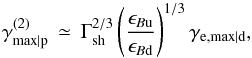9)while in model (1), where the transport is governed by the orbit of the accelerated particle in the background field, ${\mathit{\gamma }}_{\max \mathrm{|}\mathrm{p}}^{\mathrm{\left(}\mathrm{1}\mathrm{\right)}}\hspace{0.17em}\mathrm{\simeq }\hspace{0.17em}{\mathrm{\Gamma }}_{\mathrm{sh}}{\left(\frac{\mathit{\sigma }}{{\mathit{ϵ}}_{\mathit{B}\mathrm{d}}}\right)}^{\mathrm{1}\mathit{/}\mathrm{4}}{\mathit{\gamma }}_{\mathrm{e}\mathit{,}\max \mathrm{|}\mathrm{d}}^{\mathrm{Bohm}}$(10)In principle, one must also bound these maximum Lorentz factors using the condition that the upstream residence time cannot exceed the age of the shock front in the upstream frame, i.e. R/c; for the range of parameters that we consider here, however, this constraint is not significant.

For reference, the dependence of these maximum Lorentz factors on the shock parameters are (in the precursor frame)

$\begin{array}{ccc}& & \mathrm{2}{\mathrm{\Gamma }}_{\mathrm{sh}}{\mathit{\gamma }}_{\max \mathrm{|}\mathrm{d}}\mathrm{\simeq }\mathrm{2}\mathrm{\times }{\mathrm{10}}^{\mathrm{8}}\hspace{0.17em}{\mathit{E}}_{\mathrm{54}}^{\mathrm{0.1}}{\mathit{\lambda }}_{\mathit{\delta B,}\mathrm{1}}^{\mathrm{1}\mathit{/}\mathrm{3}}{\mathit{ϵ}}_{\mathit{B}\mathrm{d}\mathit{,}\mathrm{-}\mathrm{5}}^{\mathrm{0.1}}{\mathit{n}}_{\mathrm{0}}^{-0.3}{\mathit{ϵ}}_{\mathrm{e}\mathit{,}\mathrm{-}\mathrm{1}}^{-0.2}{\mathit{t}}_{\mathrm{obs}\mathit{,}\mathrm{4}}^{-0.4}{\mathit{z}}_{\mathrm{+}}^{\mathrm{0.4}}\\ & & {\mathit{\gamma }}_{\max \mathrm{|}\mathrm{p}}^{\mathrm{\left(}\mathrm{1}\mathrm{\right)}}\mathrm{\simeq }\mathrm{4}\mathrm{\times }{\mathrm{10}}^{\mathrm{8}}\hspace{0.17em}{\mathit{\sigma }}_{\mathrm{u}\mathit{,}\mathrm{-}\mathrm{9}}^{\mathrm{1}\mathit{/}\mathrm{4}}{\mathit{n}}_{\mathrm{0}}^{-0.4}{\mathit{ϵ}}_{\mathit{B}\mathrm{d}\mathit{,}\mathrm{-}\mathrm{5}}^{-0.3}{\mathit{ϵ}}_{\mathrm{e}\mathit{,}\mathrm{-}\mathrm{1}}^{-0.3}{\mathit{t}}_{\mathrm{obs}\mathit{,}\mathrm{4}}^{-0.2}{\mathit{z}}_{\mathrm{+}}^{\mathrm{0.2}}\\ & & \end{array}$(11)with z₊ ≡ (1 + z)/2. This indicates that these Lorentz factors are typically of the same order of magnitude. The above expressions assume the limit Y ≫ 1 and the Lorentz factor of the blast is related to the observer time t_obs and other standard parameters following the standard Blandford & McKee (1976) deceleration law. We recall that in model (i), it is necessary to retain the minimum of 2Γ_shγ_{e,max | d} and ${\mathit{\gamma }}_{\mathrm{e}\mathit{,}\max \mathrm{|}\mathrm{p}}^{\mathrm{\left(}\mathit{i}\mathrm{\right)}}$.

Combining the above results, it is possible to plot the synchrotron self-Compton (SSC) spectrum of the downstream radiation together with the synchrotron flux from the precursor. The inverse Compton emission is modelled with broken power laws following Sari & Esin (2001). Examples are shown in Fig. 1 for various cases of interest.

The synchrotron radiation from the precursor is indicated by the shaded area, bracketed by the two models (1) and (2) corresponding to regular deflection and radiation in a background magnetic field or to stochastic small-angle deflection and radiation in a micro-turbulent field; the lower curve corrresponds to (1), while the upper curve corresponds to (2). Equations (11) can be used to scale the maximum Lorentz factor, hence frequency, to other cases.

Fig. 1 Spectral flux per log frequency interval νFν for the downstream synchrotron emission (red), the downstream inverse Compton spectrum (purple), and the precursor synchrotron signal (shaded area). This last shaded area is bracketed by the two extreme models of regular deflection (lower curve, model (1)) or stochastic small-angle deflection (upper curve, model (2)). The parameters of the model are indicated in the figure. For panels a) and b), representative of the external shock of a long gamma-ray burst at different times, the redshift is z = 1; for panel c), representative of a low-luminosity gamma-ray burst or trans-relativistic supernova, z = 0.01.

These results indicate that the precursor contribution is dominated by the SSC spectrum of the shocked plasma in most cases considered. It appears that the only case in which this precursor can emerge is for a trans-relativistic shock, as depicted in case (c), if the micro-turbulent component dominates the scattering and the radiation up to the maximum energies. In all cases the contribution of model (1) is strongly suppressed: although the spectrum is harder than that of downstream, the maximum energy of particles remains limited by the downstream residence time and the maximum frequency emitted upstream is then suppressed by the relatively low magnetic field.

At extremely early times, the ratio Δ_i/R plays in favour of the precursor contribution. This likely explains why the precursor emission stands out clearly in the numerical simulations of Sironi & Spitkovsky (2009); in such simulations the size of the precursor is comparable to the size of the downstream shocked plasma. We also note that at the early time of these simulations, the accelerated particles concentrate in a layer in front of the shock, i.e. the precursor has not developed to a full extent with a position dependent minimum momentum; this explains the standard synchrotron spectrum seen in such simulations. We have not considered such early times in the above more realistic cases because at t_obs ≪ t_dec, where t_dec marks the onset of the decelerating Blandford & McKee (1976) solution, the overall non-thermal luminosity is suppressed by some power of t_obs/t_dec.

Finally, we discuss briefly the expected degree of polarization. Theoretical and numerical developments both suggest that the micro-turbulence in the precursor is two-dimensional isotropic, confined in the plane transverse to the shock normal (e.g. Medvedev & Loeb 1999; Spitkovsky 2008). In the precursor frame, where this turbulence is mostly of magnetic nature, the electron distribution is sharply beamed into an opening angle 1/Γ_sh. In such a configuration, the fraction of linearly polarized synchrotron radiation can be expressed as (Laing 1980) ${\mathit{p}}_{\mathrm{lin}}\hspace{0.17em}\mathrm{=}\hspace{0.17em}{\mathit{p}}_{\mathrm{lin}\mathit{,}\max }\mathit{f}{}^{\mathrm{(}}\mathit{\theta }_{{k}{{\beta }}_{\mathrm{sh}}}{}^{\mathrm{)}}$, where p_lin,max is the degree of maximum linear polarization (in a regular field) and θ_kβsh represents the angle between the direction of propagation of the photon k and the shock normal β_sh. The function f depends on the spectral index of the electron distribution; the result f(θ) = sin²θ/⁽1 + cos²θ⁾, corresponding to s = 3, is often used as an approximation. However, in our case, θ_kβsh ≲ 1/Γ_sh implies that the fraction of linear polarization is at most of order $\mathrm{1}\mathit{/}{\mathrm{\Gamma }}_{\mathrm{sh}}^{\mathrm{2}}$. This stands in contrast with the contribution from the downstream plasma, in which partial linear polarization may subsist (e.g. Nava et al. 2016). One can check that the degree of circular polarization scales in proportion to cosα_δB, where α_δB represents the angle of the (random) magnetic field in the transverse plane at a given point; consequently, this contribution vanishes in the average over α_δB. The synchrotron radiation in a Weibel-like micro-turbulent precursor is thus essentially unpolarized.

In contrast, linear polarization is maximum in the background magnetic field, with p_lin,max = [7 + 3(s−1)] / [3 + 3(s−1)] ≃ 63 % for s = 2.3 and regular deflection. This fraction is now much larger than that expected from the downstream side, even if the field were regular there, because of the averaging procedures over the viewing angles that results from the Lorentz boosting of the downstream emission, as discussed in detail in Nava et al. (2016). In principle, this offers a new way to study the precursor at the highest frequencies, where model (1) is expected to hold; unfortunately, the strong suppression of precursor emission in this model in all cases considered renders the detection of this polarized signal unlikely.

We note that the beaming of the electron distribution also produces net circular polarization in the background magnetic field. The fraction of circularly polarized synchrotron light scales as p_circ ~ 1/ ⟨ γ ⟩ dlnϕ/ dθ, where ϕ characterizes the angular part of the distribution function, θ represents the pitch angle relative to the magnetic field, and ⟨ γ ⟩ the mean Lorentz factor. In the precursor, $\mathrm{d}\ln \mathit{\varphi }\mathit{/}\mathrm{d}\mathit{\theta }\hspace{0.17em}\mathrm{~}\hspace{0.17em}\mathrm{𝒪}{}^{\mathrm{(}}\mathrm{\Gamma }_{\mathrm{sh}}{}^{\mathrm{)}}$, but ⟨ γ ⟩ ~ Γ_shγ_m implies that the overall fraction remains quite small, of order 1 /γ_m. Here as well, this contribution appears negligible; it could not, in particular, explain the amount of circular polarization inferred recently in a gamma-ray burst afterglow (Wiersema et al. 2014).

3. Synchrotron precursor of non-relativistic collisionless shock waves

The sub-relativistic flow velocities seen for example in supernovae remnants, imply no Lorentz boosting/beaming effects. This is a crucial distinction because it implies that the source can be seen off-axis, and in particular that the shock can be imaged edge-on, at its limb. Such morphological data offers the possibility of isolating the precursor contribution by concentrating on the emission in front of the shock, as sketched in Fig. 2. A major question is whether one actually sees the precursor at the limb, or some contribution from shocked plasma further behind due to some departures from spherical symmetry (Vink 2013). We leave this question aside here and compute the morphological and spectral properties of this upstream synchrotron emission assuming ideal spherical symmetry. We also neglect the contribution of bremsstrahlung emission in the X-ray domain, the domain that we are interested in here.

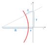Fig. 2 Sketch of the geometry for studying and computing the emission of the precursor in a non-relativistic, supernova remnant-like source. The line of sight is oriented along the y-axis.

More specifically, we compute the surface brightness of the synchrotron radiation ${\mathit{S}}_{\mathit{\nu ,}\mathrm{p}}\hspace{0.17em}\mathrm{=}\hspace{0.17em}{\mathrm{\int }}_{\mathrm{-}\mathrm{\infty }}^{\mathrm{+}\mathrm{\infty }}\mathrm{d}\mathit{y}\hspace{0.17em}\mathit{j}\nu$(12)with j_ν the position dependent emissivity in the precursor. The integration is taken along the line of sight, oriented along the y-axis (see Fig. 2). We consider a point, located a distance x in front of the shock, with x ≪ R (R the shock radius). Then, the coordinate along the line of sight can be written $\mathit{y}\hspace{0.17em}\mathrm{=}\hspace{0.17em}{{}^{\mathrm{[}}\left(\mathit{R}\mathrm{+}\mathrm{\Delta }\right)^{\mathrm{2}}\mathrm{-}{{}^{\mathrm{(}}\mathit{R}\mathrm{+}{\mathit{x}}^{\mathrm{)}}}^{\mathrm{2}}{}^{\mathrm{]}}}^{\mathrm{1}\mathit{/}\mathrm{2}}\hspace{0.17em}\mathrm{\simeq }\hspace{0.17em}{\left[\mathrm{2}\mathrm{(}\mathrm{\Delta }\mathrm{-}\mathit{x}\mathrm{)}\mathit{R}\right]}^{\mathrm{1}\mathit{/}\mathrm{2}}$ in terms of the depth Δ in the precursor, measured relative to the shock front radius, as indicated in Fig. 2. The integral in Eq. (15) thus samples depths in the precursor Δ ∈ [ x, + ∞ [, with differing contributions to the emissivity at a given frequency.

We model the distribution function of electrons in the precursor as $\frac{\mathrm{d}{\mathit{n}}_{\mathrm{e}}\mathrm{\left(}\mathrm{\Delta }\mathrm{\right)}}{\mathrm{d}\mathit{p}}\hspace{0.17em}\mathrm{\simeq }\hspace{0.17em}\frac{{\mathit{n}}_{\mathrm{e}}}{{\mathit{p}}_{\min }}{\left(\frac{\mathit{p}}{{\mathit{p}}_{\min }}\right)}^{\mathrm{-}\mathit{s}}\exp \left(\mathrm{-}\frac{\mathit{p}}{{\mathit{p}}_{\max }}\right)\exp \left[\mathrm{-}\frac{\mathrm{\Delta }}{{\mathit{r}}_{\mathrm{p}}\mathrm{\left(}\mathit{p}\mathrm{\right)}}\right]$(13)in terms of the minimum (p_min) and maximum (p_max) momenta of the distribution. As before, r_p(p) represents the typical length scale of the precursor for particles of momentum p. While the dependence ∝exp(−x/r_p) represents the generic solution of the diffusion–advection equation in a uniform turbulence (see e.g. Drury 1983), the dependence ∝exp(−p/p_max) is phenomenological. The results derived below can be extended to other cut-off forms discussed in Zirakashvili & Aharonian (2007).

The precursor length scale is defined by r_p ≃ ct_scatt/β_sh in terms of the scattering time and shock velocity. For a turbulence of homogeneous strength and Bohm scaling of the scattering frequency, this length scale is r_p(p) ≃ r_g/β_sh, with r_g = pc/ (eB_p) the gyroradius and B_p the magnetic field strength in the precursor; for Kolmogorov-type (homogeneous) turbulence, however, ${\mathit{r}}_{\mathrm{p}}\hspace{0.17em}\mathrm{\simeq }\hspace{0.17em}{\mathit{\lambda }}_{\max }^{\mathrm{2}\mathit{/}\mathrm{3}}{\mathit{r}}_{\mathrm{g}}^{\mathrm{1}\mathit{/}\mathrm{3}}\mathit{/}{\mathit{\beta }}_{\mathrm{sh}}$ (e.g. Casse et al. 2002), with λ_max the length scale of the turbulence. In order to allow a possible deviation from a Bohm scaling, we adopt a phenomenological scaling r_p ∝ p^{1/(1 + α_λ)} (i.e. α_λ = (0,2) for homogeneous Bohm or Kolmogorov-type scalings, respectively). It may be useful to recall that in a generic turbulence of scale λ_max, particles of gyroradius r_g ~ λ_max indeed scatter at a rate close to Bohm, but particles of much smaller gyroradius may scatter at a quite different rate.

It might also be possible to take into account a spatial dependence of the magnetic field strength in the precursor. However, modelling of supernova remnants suggests that the pre-shock amplification factor of the background magnetic field is of the order of a factor of ten (e.g. Berezhko et al. 2003). Therefore, such dependence, if it exists, is likely to be quite mild. In the following, we assume that on the scales probed by the electrons, the magnetic field strength is uniform in the precursor, but we allow for a possible additional amplification of the latter in the shock transition.

We write the synchrotron spectral power of one electron as ${\mathit{r}}_{\mathit{\nu }}\exp \mathrm{(}\mathrm{-}\mathit{\nu }\mathit{/}{\mathit{\nu }}_{\mathrm{c}}\mathrm{)}\sqrt{\mathrm{3}}{\mathit{e}}^{\mathrm{3}}{\mathit{B}}_{\mathrm{p}}\mathit{/}\mathrm{\left(}{\mathit{m}}_{\mathrm{e}}{\mathit{c}}^{\mathrm{2}}\mathrm{\right)}$ with ν_c ∝ p² the synchrotron peak frequency; the function r_ν ≃ (ν/ν_c)^1/3 at ν ≪ ν_c and r_ν ~ 1 at ν ≳ ν_c, see Eq. (30) of Zirakashvili & Aharonian (2007).

Noting that 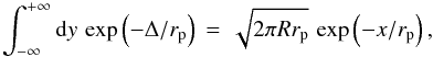${\mathrm{\int }}_{\mathrm{-}\mathrm{\infty }}^{\mathrm{+}\mathrm{\infty }}\mathrm{d}\mathit{y}\hspace{0.17em}\exp \mathrm{(}\mathrm{-}\mathrm{\Delta }\mathit{/}{\mathit{r}}_{\mathrm{p}}\mathrm{)}\hspace{0.17em}\mathrm{=}\hspace{0.17em}\sqrt{\mathrm{2}\mathit{\pi R}{\mathit{r}}_{\mathrm{p}}}\hspace{0.17em}\exp \mathrm{(}\mathrm{-}\mathit{x}\mathit{/}{\mathit{r}}_{\mathrm{p}}\mathrm{)}\mathit{,}$(14)the surface brightness at position x> 0 can be written 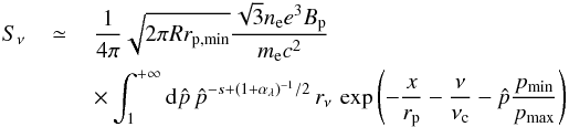$\begin{array}{ccc}{\mathit{S}}_{\mathit{\nu }}& \hspace{0.17em}\mathrm{\simeq }\hspace{0.17em}& \frac{\mathrm{1}}{\mathrm{4}\mathit{\pi }}\sqrt{\mathrm{2}\mathit{\pi R}{\mathit{r}}_{\mathrm{p}\mathit{,}\min }}\frac{\sqrt{\mathrm{3}}{\mathit{n}}_{\mathrm{e}}{\mathit{e}}^{\mathrm{3}}{\mathit{B}}_{\mathrm{p}}}{{\mathit{m}}_{\mathrm{e}}{\mathit{c}}^{\mathrm{2}}}\\ & & \mathrm{\times }{\mathrm{\int }}_{\mathrm{1}}^{\mathrm{+}\mathrm{\infty }}\mathrm{d}\mathit{p̂}\hspace{0.17em}\mathit{p̂}\mathrm{-}\mathit{s}\mathrm{+}\mathrm{(}\mathrm{1}\mathrm{+}{\mathit{\alpha }}_{\mathit{\lambda }}{\mathrm{)}}^{-1}\mathit{/}\mathrm{2}\hspace{0.17em}{\mathit{r}}_{\mathit{\nu }}\hspace{0.17em}\exp \left(\mathrm{-}\frac{\mathit{x}}{{\mathit{r}}_{\mathrm{p}}}\mathrm{-}\frac{\mathit{\nu }}{{\mathit{\nu }}_{\mathrm{c}}}\mathrm{-}\mathit{p̂}\frac{{\mathit{p}}_{\min }}{{\mathit{p}}_{\max }}\right)\\ & & \end{array}$(15)with , r_p,min ≡ r_p(p_min). The exponent (1 + α_λ)^-1/ 2 arises through the effective depth of integration on the line of sight and its momentum dependence. In the following, we use the short-hand notation: ${\mathit{s}}_{\mathrm{0}}\hspace{0.17em}\mathrm{\equiv }\hspace{0.17em}{{}^{\mathrm{[}}\mathit{R}{\mathit{r}}_{\mathrm{p}\mathit{,}\min }\mathit{/}\mathrm{(}\mathrm{2}\mathit{\pi }{\mathrm{\left)}}^{\mathrm{\right]}}}^{\mathrm{1}\mathit{/}\mathrm{2}}\sqrt{\mathrm{3}}{\mathit{n}}_{\mathrm{e}}{\mathit{e}}^{\mathrm{3}}{\mathit{B}}_{\mathrm{p}}\mathit{/}\mathrm{\left(}{\mathit{m}}_{\mathrm{e}}{\mathit{c}}^{\mathrm{2}}\mathrm{\right)}$.

The integral in Eq. (15) can be integrated in various limits. Consider first the case x ≪ r_p(p_ν) and ν ≪ ν_max with ν_max ≡ ν_c(p_max). Here, p_ν is understood as the momentum for which the synchrotron peak frequency equals ν and it should not be confused with the spectral power of an electron, i.e. ν_c(p_ν) ≡ ν. The above limit then means that at location x, electrons radiate at their peak frequency at ν; consequently, the spectrum at ν will be shaped by these electrons. The limit x ≪ r_p(p_ν) implies exp⁽−x/r_p⁾ ~ 1 in the range of momenta which contribute to the radiation at ν, hence this exponential dependence can be safely ignored. This results in a usual integration of the synchrotron spectral power over a powerlaw distribution, albeit with a modified index s−(1 + α_λ)^-1/ 2, which leads to the result (omitting numerical prefactors of the order of unity) ${\mathit{S}}_{\mathit{\nu }}\hspace{0.17em}\mathrm{\simeq }\hspace{0.17em}{\mathit{s}}_{\mathrm{0}}{\left(\frac{\mathit{\nu }}{{\mathit{\nu }}_{\min }}\right)}^{\mathrm{(}\mathrm{1}\mathrm{-}\mathit{s}\mathrm{)}\mathit{/}\mathrm{2}\mathrm{+}\mathrm{(}\mathrm{1}\mathrm{+}{\mathit{\alpha }}_{\mathit{\lambda }}{\mathrm{)}}^{-1}\mathit{/}\mathrm{4}} \mathrm{[}\mathit{x}\hspace{0.17em}\mathrm{\ll }\hspace{0.17em}{\mathit{r}}_{\mathrm{p}}\mathrm{(}{\mathit{p}}_{\mathit{\nu }}{\mathrm{\left)}}^{\mathrm{\right]}}\mathit{.}$(16)We note that the constraint x ≪ r_p(p_ν) can also be rewritten ν ≫ ν_<(x) with ν_<(x) defined implicitly by r_p[p_ν<(x)] = x. Its meaning is the following: at distance x, the electron distribution has an effective low-energy cut-off at p such that r_p(p) = x because particles of smaller momenta cover smaller distances in the precursor; hence, the local minimum synchrotron frequency of this population is ν_<(x).

We consider now the limit x ≫ r_p(p_ν), with still ν ≪ ν_max. In this limit, ν ≪ ν_<(x), hence at all Δ >x, we collect at ν only the low-frequency tail ∝ν^1/3 of the spectral flux of high-energy particles. To model the flux in this limit, it is possible to make the approximation $\exp {}^{\mathrm{(}}\mathrm{-}\mathit{x}\mathit{/}{\mathit{r}}_{\mathrm{p}}{}^{\mathrm{)}}\hspace{0.17em}\mathrm{~}\hspace{0.17em}\mathrm{\Theta }{}^{\mathrm{(}}\mathit{r}_{\mathrm{p}}\mathrm{-}{\mathit{x}}^{\mathrm{)}}$ as in Sect. 2. This Heaviside function in x effectively constrains the range of integration, i.e. Eq. (15) can be rewritten $\begin{array}{ccc}{\mathit{S}}_{\mathit{\nu }}& \hspace{0.17em}\mathrm{\simeq }\hspace{0.17em}& {\mathit{s}}_{\mathrm{0}}\hspace{0.17em}{\mathrm{\int }}_{\mathrm{(}\mathit{x}\mathit{/}{\mathit{r}}_{\mathrm{p}\mathit{,}\min }{\mathrm{)}}^{\mathrm{(}\mathrm{1}\mathrm{+}{\mathit{\alpha }}_{\mathit{\lambda }}\mathrm{)}}}^{\mathrm{+}\mathrm{\infty }}\mathrm{d}\mathit{p̂}\hspace{0.17em}\mathit{p̂}\mathrm{-}\mathit{s}\mathrm{+}\mathrm{(}\mathrm{1}\mathrm{+}{\mathit{\alpha }}_{\mathit{\lambda }}{\mathrm{)}}^{-1}\mathit{/}\mathrm{2}\hspace{0.17em}{\left(\frac{\mathit{\nu }}{{\mathit{\nu }}_{\mathrm{c}}}\right)}^{\mathrm{1}\mathit{/}\mathrm{3}}\\ & \hspace{0.17em}\mathrm{\simeq }\hspace{0.17em}& {\mathit{s}}_{\mathrm{0}}\hspace{0.17em}{\left(\frac{\mathit{x}}{{\mathit{r}}_{\mathrm{p}\mathit{,}\min }}\right)}^{\left(\frac{\mathrm{1}}{\mathrm{3}}\mathrm{-}\mathit{s}\right)\mathrm{(}\mathrm{1}\mathrm{+}{\mathit{\alpha }}_{\mathit{\lambda }}\mathrm{)}\mathrm{+}\frac{\mathrm{1}}{\mathrm{2}}}{\left(\frac{\mathit{\nu }}{{\mathit{\nu }}_{\min }}\right)}^{\mathrm{1}\mathit{/}\mathrm{3}} \mathrm{[}\mathit{x}\hspace{0.17em}\mathrm{\gg }\hspace{0.17em}{\mathit{r}}_{\mathrm{p}}\mathrm{(}{\mathit{p}}_{\mathit{\nu }}{\mathrm{)}}^{\mathrm{]}}\mathit{.}\\ & & \end{array}$(17)To summarize, the general spectro-morphological aspect of the synchrotron surface brightness of the precursor well below the maximum frequency ν_max is given by the conjunction of Eqs. (16) and (17). At x ≪ r_p(p_ν), the surface brightness is constant in x with a harder than usual spectrum in ν, then decreases according to Eq. (17) at x ≫ r_p(p_ν), e.g. ∝x^{− 7/6} for s = 2 and α_λ = 0.

As we will see, the detection of the precursor becomes promising only at the highest frequencies, which, for typical supernovae remnants, fall in the X-ray range. Indeed, electrons radiating at ν at their synchrotron peak frequency have an energy ${\mathit{ϵ}}_{\mathrm{e}}\hspace{0.17em}\mathrm{\simeq }\hspace{0.17em}\mathrm{10}\hspace{0.17em}\mathrm{TeV}\hspace{0.17em}\mathrm{(}\mathit{h\nu }\mathit{/}\mathrm{1}\hspace{0.17em}\mathrm{keV}{\mathrm{)}}^{\mathrm{1}\mathit{/}\mathrm{2}}{\mathit{n}}_{\mathrm{0}}^{\mathrm{-}\mathrm{1}\mathit{/}\mathrm{4}}{\mathit{\beta }}_{\mathrm{sh}\mathit{,}\mathrm{-}\mathrm{1.5}}^{\mathrm{-}\mathrm{1}\mathit{/}\mathrm{2}}{\mathit{ϵ}}_{\mathit{B}\mathrm{p}\mathit{,}\mathrm{-}\mathrm{3}}^{\mathrm{-}\mathrm{1}\mathit{/}\mathrm{4}}$, where ${\mathit{ϵ}}_{\mathit{B}\mathrm{p}}\hspace{0.17em}\mathrm{\equiv }\hspace{0.17em}{\mathit{B}}_{\mathrm{p}}^{\mathrm{2}}\mathit{/}{}^{\mathrm{(}}\mathrm{4}\mathit{\pi nm}{\mathit{\beta }}_{\mathrm{sh}}^{\mathrm{2}}{\mathit{c}}^{\mathrm{2}}{}^{\mathrm{)}}$. As for the maximum energy of accelerated electrons, balancing synchrotron cooling with the acceleration time scale t_acc = κr_p/ (β_shc), we find 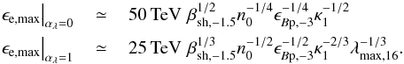$\begin{array}{ccc}{{\mathit{ϵ}}_{\mathrm{e}\mathit{,}\max }|}_{{\mathit{\alpha }}_{\mathit{\lambda }}\mathrm{=}\mathrm{0}}& \hspace{0.17em}\mathrm{\simeq }\hspace{0.17em}& \mathrm{50}\hspace{0.17em}\mathrm{TeV}\hspace{0.17em}\hspace{0.17em}{\mathit{\beta }}_{\mathrm{sh}\mathit{,}\mathrm{-}\mathrm{1.5}}^{\mathrm{1}\mathit{/}\mathrm{2}}{\mathit{n}}_{\mathrm{0}}^{\mathrm{-}\mathrm{1}\mathit{/}\mathrm{4}}{\mathit{ϵ}}_{\mathit{B}\mathrm{p}\mathit{,}\mathrm{-}\mathrm{3}}^{\mathrm{-}\mathrm{1}\mathit{/}\mathrm{4}}{\mathit{\kappa }}_{\mathrm{1}}^{\mathrm{-}\mathrm{1}\mathit{/}\mathrm{2}}\\ {{\mathit{ϵ}}_{\mathrm{e}\mathit{,}\max }|}_{{\mathit{\alpha }}_{\mathit{\lambda }}\mathrm{=}\mathrm{1}}& \hspace{0.17em}\mathrm{\simeq }\hspace{0.17em}& \mathrm{25}\hspace{0.17em}\mathrm{TeV}\hspace{0.17em}\hspace{0.17em}{\mathit{\beta }}_{\mathrm{sh}\mathit{,}\mathrm{-}\mathrm{1.5}}^{\mathrm{1}\mathit{/}\mathrm{3}}{\mathit{n}}_{\mathrm{0}}^{\mathrm{-}\mathrm{1}\mathit{/}\mathrm{2}}{\mathit{ϵ}}_{\mathit{B}\mathrm{p}\mathit{,}\mathrm{-}\mathrm{3}}^{\mathrm{-}\mathrm{1}\mathit{/}\mathrm{2}}{\mathit{\kappa }}_{\mathrm{1}}^{\mathrm{-}\mathrm{2}\mathit{/}\mathrm{3}}{\mathit{\lambda }}_{\max \mathit{,}\mathrm{16}}^{\mathrm{-}\mathrm{1}\mathit{/}\mathrm{3}}\mathit{.}\end{array}$(18)It is thus necessary to compute the spectrum close to ν_max and at distances x ~ r_p,max${}^{\mathrm{[}}\mathit{r}_{\mathrm{p}\mathit{,}\max }\hspace{0.17em}\mathrm{\equiv }\hspace{0.17em}{\mathit{r}}_{\mathrm{p}}\mathrm{(}{\mathit{p}}_{\max }{\mathrm{\left)}}^{\mathrm{\right]}}$. In this limit, the exponential turn-over of the electron distribution in momentum and in distance must be retained as the exponential turn-over of the synchrotron spectral power. It is possible nevertheless obtain a reasonable approximation to S_ν through a saddle-point approximation of the integral. To this effect, we define $\mathit{g}\mathrm{\left(}\mathit{p}\mathrm{\right)}\hspace{0.17em}\mathrm{=}\hspace{0.17em}\frac{\mathit{x}}{{\mathit{r}}_{\mathrm{p}}}\mathrm{+}\frac{\mathit{\nu }}{{\mathit{\nu }}_{\mathrm{c}}}\mathrm{+}\frac{\mathit{p}}{{\mathit{p}}_{\max }}$(19)and p_⋆ such that g′(p_⋆) = 0. Then $\begin{array}{ccc}{\mathit{S}}_{\mathit{\nu }}& \hspace{0.17em}\mathrm{\simeq }\hspace{0.17em}& {\mathit{s}}_{\mathrm{0}}{\left(\frac{{\mathit{p}}_{\mathit{\star }}}{{\mathit{p}}_{\min }}\right)}^{\mathrm{1}\mathrm{-}\mathit{s}\mathrm{+}\mathrm{(}\mathrm{1}\mathrm{+}{\mathit{\alpha }}_{\mathit{\lambda }}{\mathrm{)}}^{-1}\mathit{/}\mathrm{2}}\sqrt{\frac{\mathrm{2}\mathit{\pi }}{{\mathit{g}}_{\mathit{\star }}^{\mathrm{\prime \prime }}}}{\mathit{r}}_{\mathit{\nu }}\mathrm{\left(}{\mathit{p}}_{\mathit{\star }}\mathrm{\right)}\hspace{0.17em}{\mathit{e}}^{\mathrm{-}{\mathit{g}}_{\mathit{\star }}}\\ & & \end{array}$(20)with the short-hand notations: g_⋆ ≡ g(p_⋆), g″_⋆ = g″(p_⋆). In the limits x ≳ r_p,max ∧ ν ≪ ν_max, or x ≪ r_p,max ∧ ν ≳ ν_max, the following approximate solutions can be used: $\begin{array}{ccc}{\mathit{p}}_{\mathit{\star }}& \hspace{0.17em}\mathrm{\simeq }\hspace{0.17em}& {\mathit{p}}_{\max }\hspace{0.17em}\hspace{0.17em}\max \left[\mathrm{1.2}{\left(\frac{\mathit{\nu }}{{\mathit{\nu }}_{\max }}\right)}^{\mathrm{1}\mathit{/}\mathrm{3}}\mathit{,}\hspace{0.17em}\hspace{0.17em}{\mathit{a}}_{\mathit{\lambda }}{\left(\frac{\mathit{x}}{{\mathit{r}}_{\mathrm{p}\mathit{,}\max }}\right)}^{\mathrm{(}\mathrm{1}\mathrm{+}{\mathit{\alpha }}_{\mathit{\lambda }}\mathrm{)}\mathit{/}\mathrm{(}\mathrm{2}\mathrm{+}{\mathit{\alpha }}_{\mathit{\lambda }}\mathrm{)}}\right]\\ {\mathit{g}}_{\mathit{\star }}& \hspace{0.17em}\mathrm{\simeq }\hspace{0.17em}& \max \left[\mathrm{1.9}{\left(\frac{\mathit{\nu }}{{\mathit{\nu }}_{\max }}\right)}^{\mathrm{1}\mathit{/}\mathrm{3}}\mathit{,}\hspace{0.17em}\hspace{0.17em}{\mathit{b}}_{\mathit{\lambda }}{\left(\frac{\mathit{x}}{{\mathit{r}}_{\mathrm{p}\mathit{,}\max }}\right)}^{\mathrm{(}\mathrm{1}\mathrm{+}{\mathit{\alpha }}_{\mathit{\lambda }}\mathrm{)}\mathit{/}\mathrm{(}\mathrm{2}\mathrm{+}{\mathit{\alpha }}_{\mathit{\lambda }}\mathrm{)}}\right]\\ {\mathit{g}}_{\mathit{\star }}^{\mathrm{\prime \prime }}& \hspace{0.17em}\mathrm{\simeq }\hspace{0.17em}& \end{array}$(21)with a_λ = (1 + α_λ)^{− (1 + α_λ)/(2 + α_λ)}, b_λ = (1 + α_λ)^{1/(2 + α_λ)} + a_λ, and c_λ = (2 + α_λ)(1 + α_λ)^{− 1/(2 + α_λ)}. With these approximate scalings, Eq. (20) provides the leading order approximation to the spectro-morphological shape of the precursor emission at high frequency and/or great distance. It indicates in particular that the precursor emission can extend up to a few times r_p,max with a rather smooth exponential decay beyond.

The contribution from the shocked plasma exists only at negative values of x. At a given x, the (homogeneous) contribution of this shocked plasma is integrated up to an effective depth along the line of sight $\mathit{y}\hspace{0.17em}\mathrm{\simeq }\hspace{0.17em}\sqrt{\mathrm{2}\mathit{R}\mathrm{\left|}\mathit{x}\mathrm{\right|}}$ for | x | ≪ R. Repeating the above integrations, the downstream surface brightness can thus be written as ${\mathit{S}}_{\mathit{\nu ,}\mathrm{d}}\hspace{0.17em}\mathrm{\simeq }\hspace{0.17em}{\mathit{r}}_{\mathrm{amp}}^{\mathrm{(}\mathit{s}\mathrm{+}\mathrm{1}\mathrm{)}\mathit{/}\mathrm{2}}\hspace{0.17em}{\mathit{s}}_{\mathrm{0}}\hspace{0.17em}{\left(\frac{\mathrm{\left|}\mathit{x}\mathrm{\right|}}{{\mathit{x}}_{\min }}\right)}^{\mathrm{1}\mathit{/}\mathrm{2}}\hspace{0.17em}{\left[\frac{\mathit{\nu }}{{\mathit{\nu }}_{\min }}\right]}^{\mathrm{(}\mathrm{1}\mathrm{-}\mathit{s}\mathrm{)}\mathit{/}\mathrm{2}} \mathrm{[}\mathit{\nu }\hspace{0.17em}\mathrm{\ll }\hspace{0.17em}{\mathit{r}}_{\mathrm{amp}}{\mathit{\nu }}_{\max }\mathrm{]}\mathit{.}$(22)The first term on the right-hand side, with r_amp ≃ 4A_amp, contains both the compression ratio at the shock (4) and a possible amplification factor due to the non-linear processing downstream of the shock (A_amp). The corresponding exponent (s + 1)/2 arises because the spectrum has been expressed in terms of ν/ν_min, with ν_min the minimum frequency in the pre-shock magnetic field. The above expression should cut off beyond the cooling length l_cool of particles radiating at frequency ν. As discussed in Berezhko & Völk (2004), ${\mathit{l}}_{\mathrm{cool}}\hspace{0.17em}\mathrm{\simeq }\hspace{0.17em}\max {}^{\mathrm{[}}\sqrt{{\mathit{l}}_{\mathrm{d}}{\mathit{l}}_{\mathrm{c}}}\mathit{,}{\mathit{l}}_{\mathrm{c}}{}^{\mathrm{]}}$ in terms of the downstream diffusive length scale l_d ≃ l_scatt/β_d (β_d = β_sh/ 4 the downstream shock velocity), l_scatt the mean free path, and l_c = β_dct_cool the convective cooling length scale.

In the turn-over regime, ν ≳ r_ampν_max is derived $\begin{array}{ccc}{\mathit{S}}_{\mathit{\nu ,}\mathrm{d}}& \hspace{0.17em}\mathrm{\simeq }\hspace{0.17em}& {\mathit{r}}_{\mathrm{amp}}\hspace{0.17em}{\mathit{s}}_{\mathrm{0}}\hspace{0.17em}{\left(\frac{\mathrm{\left|}\mathit{x}\mathrm{\right|}}{{\mathit{x}}_{\min }}\right)}^{\mathrm{1}\mathit{/}\mathrm{2}}\hspace{0.17em}{\left(\frac{{\mathit{p}}_{\mathit{\star }\mathit{,}\mathrm{d}}}{{\mathit{p}}_{\min }}\right)}^{\mathrm{1}\mathrm{-}\mathit{s}}\sqrt{\frac{\mathrm{2}\mathit{\pi }}{{\mathit{g}}_{\mathit{\star }\mathit{,}\mathrm{d}}^{\mathrm{\prime \prime }}}}{\mathit{r}}_{\mathit{\nu }}\mathrm{\left(}{\mathit{p}}_{\mathit{\star }\mathit{,}\mathrm{d}}\mathrm{\right)}\hspace{0.17em}{\mathit{e}}^{\mathrm{-}{\mathit{g}}_{\mathit{\star }\mathit{,}\mathrm{d}}}\\ & & \end{array}$(23)and p_⋆,d, g_⋆,d, and g″_⋆,d can be obtained in the same way as their upstream counterparts in Eq. (21), with the replacements x → 0, α_λ → 0, and ν_max → r_ampν_max.

Figure 3 presents examples of the morphological dependence of the precursor which illustrate the above scalings. In these figures, the synchrotron cooling of high-energy particles on the downstream side has been explicitly taken into account using the spatial profile described in Berezhko & Völk (2004).

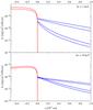Fig. 3 Surface brightness along the line of sight to the limb of a non-relativistic shock as a function of distance x to the shock, for various cases as shown: upper panel at hν = 1 keV, lower panel at hν = 10 keV. The solid lines present a complete numerical evaluation of Eq. (15), while the dotted lines correspond to the analytical approximation in the turn-over regime. Two models are shown for the precursor emission: αλ = 1 for the upper lines, i.e. tscatt ∝ p1/2, and αλ = 0 for the lower lines, i.e. Bohm scaling tscatt ∝ p. In all cases, βsh = 1/30, nu = 1 cm-3, R = 1 pc, ϵBp = 0.001, and ϵe = 0.01.

Figure 3 indicates that the contribution from the precursor is sizeable at the highest frequencies, especially if maximum energy electrons scatter more slowly than the Bohm scaling. To put things in proper perspective, recall that 1″ resolution at a distance of 1 kpc corresponds to a spatial resolution of 1.4 × 10¹⁶cm, which provides a reasonable approximation to the extent of the precursor emission r_p,max. If the magnetic field were to receive substantial amplification in the near precursor, i.e. at distances x ≪ r_p,max, the synchrotron contribution of the precursor would be accordingly reduced.

Using Eqs. (16), (17), (20), (22), and (23), it is possible to compare the emission of the precursor relative to that of downstream. In the inertial range ν ≪ ν_max, the ratio of the upstream contribution, at its maximum, relative to the downstream contribution, is of order ${\mathit{r}}_{\mathrm{amp}}^{\mathrm{-}\mathrm{(}\mathit{s}\mathrm{+}\mathrm{1}\mathrm{)}\mathit{/}\mathrm{2}}{{}^{\mathrm{[}}\mathit{r}_{\mathrm{p}}\mathrm{\left(}{\mathit{p}}_{\mathit{\nu }}\mathrm{\right)}\mathit{/}{\mathit{l}}_{\mathrm{cool}}{}^{\mathrm{]}}}^{\mathrm{1}\mathit{/}\mathrm{2}}$. In the turn-over regime, ν ≳ ν_max, this ratio becomes of the order of ${\mathit{r}}_{\mathrm{amp}}^{-1}{{}^{\mathrm{[}}\mathit{r}_{\mathrm{p}\mathit{,}\max }\mathit{/}{\mathit{l}}_{\mathrm{cool}}{}^{\mathrm{]}}}^{\mathrm{1}\mathit{/}\mathrm{2}}$ up to a factor of the order of unity which is related to the difference of exp(−g_⋆) between upstream and downstream.

For reference, 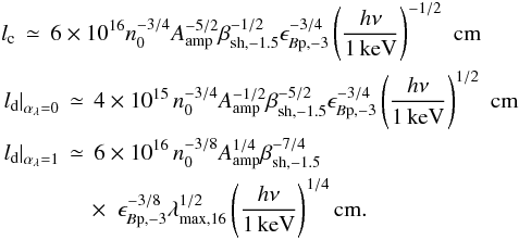$\begin{array}{ccc}& & {\mathit{l}}_{\mathrm{c}}\hspace{0.17em}\mathrm{\simeq }\hspace{0.17em}\mathrm{6}\mathrm{\times }{\mathrm{10}}^{\mathrm{16}}{\mathit{n}}_{\mathrm{0}}^{\mathrm{-}\mathrm{3}\mathit{/}\mathrm{4}}{\mathit{A}}_{\mathrm{amp}}^{\mathrm{-}\mathrm{5}\mathit{/}\mathrm{2}}{\mathit{\beta }}_{\mathrm{sh}\mathit{,}\mathrm{-}\mathrm{1.5}}^{\mathrm{-}\mathrm{1}\mathit{/}\mathrm{2}}{\mathit{ϵ}}_{\mathit{B}\mathrm{p}\mathit{,}\mathrm{-}\mathrm{3}}^{\mathrm{-}\mathrm{3}\mathit{/}\mathrm{4}}{\left(\frac{\mathit{h\nu }}{\mathrm{1}\hspace{0.17em}\mathrm{keV}}\right)}^{\mathrm{-}\mathrm{1}\mathit{/}\mathrm{2}}\hspace{0.17em}\hspace{0.17em}\mathrm{cm}\\ & & {{\mathit{l}}_{\mathrm{d}}|}_{{\mathit{\alpha }}_{\mathit{\lambda }}\mathrm{=}\mathrm{0}}\hspace{0.17em}\mathrm{\simeq }\hspace{0.17em}\mathrm{4}\mathrm{\times }{\mathrm{10}}^{\mathrm{15}}\hspace{0.17em}{\mathit{n}}_{\mathrm{0}}^{\mathrm{-}\mathrm{3}\mathit{/}\mathrm{4}}{\mathit{A}}_{\mathrm{amp}}^{\mathrm{-}\mathrm{1}\mathit{/}\mathrm{2}}{\mathit{\beta }}_{\mathrm{sh}\mathit{,}\mathrm{-}\mathrm{1.5}}^{\mathrm{-}\mathrm{5}\mathit{/}\mathrm{2}}{\mathit{ϵ}}_{\mathit{B}\mathrm{p}\mathit{,}\mathrm{-}\mathrm{3}}^{\mathrm{-}\mathrm{3}\mathit{/}\mathrm{4}}{\left(\frac{\mathit{h\nu }}{\mathrm{1}\hspace{0.17em}\mathrm{keV}}\right)}^{\mathrm{1}\mathit{/}\mathrm{2}}\hspace{0.17em}\hspace{0.17em}\mathrm{cm}\\ & & {{\mathit{l}}_{\mathrm{d}}|}_{{\mathit{\alpha }}_{\mathit{\lambda }}\mathrm{=}\mathrm{1}}\hspace{0.17em}\mathrm{\simeq }\hspace{0.17em}\mathrm{6}\mathrm{\times }{\mathrm{10}}^{\mathrm{16}}\hspace{0.17em}{\mathit{n}}_{\mathrm{0}}^{\mathrm{-}\mathrm{3}\mathit{/}\mathrm{8}}{\mathit{A}}_{\mathrm{amp}}^{\mathrm{1}\mathit{/}\mathrm{4}}{\mathit{\beta }}_{\mathrm{sh}\mathit{,}\mathrm{-}\mathrm{1.5}}^{\mathrm{-}\mathrm{7}\mathit{/}\mathrm{4}}\\ & & \end{array}$(24)Furthermore,

$\begin{array}{ccc}& & {{\mathit{r}}_{\mathrm{p}}\mathrm{\left(}{\mathit{p}}_{\mathit{\nu }}\mathrm{\right)}|}_{{\mathit{\alpha }}_{\mathit{\lambda }}\mathrm{=}\mathrm{0}}\mathrm{\simeq }\mathrm{0.7}\mathrm{\times }{\mathrm{10}}^{\mathrm{16}}\hspace{0.17em}{\mathit{n}}_{\mathrm{0}}^{\mathrm{-}\mathrm{3}\mathit{/}\mathrm{4}}{\mathit{\beta }}_{\mathrm{sh}\mathit{,}\mathrm{-}\mathrm{1.5}}^{\mathrm{-}\mathrm{5}\mathit{/}\mathrm{2}}{\mathit{ϵ}}_{\mathit{B}\mathrm{p}\mathit{,}\mathrm{-}\mathrm{3}}^{\mathrm{-}\mathrm{3}\mathit{/}\mathrm{4}}{\left(\frac{\mathit{h\nu }}{\mathrm{1}\hspace{0.17em}\mathrm{keV}}\right)}^{\mathrm{1}\mathit{/}\mathrm{2}}\hspace{0.17em}\hspace{0.17em}\mathrm{cm}\\ & & {{\mathit{r}}_{\mathrm{p}}\mathrm{\left(}{\mathit{p}}_{\mathit{\nu }}\mathrm{\right)}|}_{{\mathit{\alpha }}_{\mathit{\lambda }}\mathrm{=}\mathrm{1}}\mathrm{\simeq }\mathrm{5}\mathrm{\times }{\mathrm{10}}^{\mathrm{16}}\hspace{0.17em}{\mathit{n}}_{\mathrm{0}}^{\mathrm{-}\mathrm{3}\mathit{/}\mathrm{8}}{\mathit{\beta }}_{\mathrm{sh}\mathit{,}\mathrm{-}\mathrm{1.5}}^{\mathrm{-}\mathrm{7}\mathit{/}\mathrm{4}}{\mathit{ϵ}}_{\mathit{B}\mathrm{p}\mathit{,}\mathrm{-}\mathrm{3}}^{\mathrm{-}\mathrm{3}\mathit{/}\mathrm{8}}{\mathit{\lambda }}_{\max \mathit{,}\mathrm{16}}^{\mathrm{1}\mathit{/}\mathrm{2}}{\left(\frac{\mathit{h\nu }}{\mathrm{1}\hspace{0.17em}\mathrm{keV}}\right)}^{\mathrm{1}\mathit{/}\mathrm{4}}\mathrm{cm}\\ & & {{\mathit{r}}_{\mathrm{p}\mathit{,}\max }|}_{{\mathit{\alpha }}_{\mathit{\lambda }}\mathrm{=}\mathrm{0}}\mathrm{\simeq }\mathrm{3.6}\mathrm{\times }{\mathrm{10}}^{\mathrm{16}}{\mathit{n}}_{\mathrm{0}}^{\mathrm{-}\mathrm{3}\mathit{/}\mathrm{4}}{\mathit{\beta }}_{\mathrm{sh}\mathit{,}\mathrm{-}\mathrm{1.5}}^{\mathrm{-}\mathrm{3}\mathit{/}\mathrm{2}}{\mathit{ϵ}}_{\mathit{B}\mathrm{p}\mathit{,}\mathrm{-}\mathrm{3}}^{\mathrm{-}\mathrm{3}\mathit{/}\mathrm{4}}{\mathit{\kappa }}_{\mathrm{1}}^{\mathrm{-}\mathrm{1}\mathit{/}\mathrm{2}}\hspace{0.17em}\hspace{0.17em}\mathrm{cm}\\ & & \end{array}$(25)The “post-precursor” amplification factor A_amp exerts two opposite influences on the relative magnitude of the precursor emission: if A_amp> 1, the downstream cooling length decreases (${\mathit{l}}_{\mathrm{c}}\hspace{0.17em}\mathrm{\propto }\hspace{0.17em}{\mathit{A}}_{\mathrm{amp}}^{\mathrm{-}\mathrm{5}\mathit{/}\mathrm{2}}$ and ${\mathit{l}}_{\mathrm{d}}\hspace{0.17em}\mathrm{\propto }\hspace{0.17em}{\mathit{A}}_{\mathrm{amp}}^{\mathrm{-}\mathrm{1}\mathit{/}\mathrm{2}}$), which effectively reduces the depth of integration of the downstream emission on the line of sight, but in the meantime the downstream emissivity increases by a factor ${\mathit{A}}_{\mathrm{amp}}^{\mathrm{3}\mathit{/}\mathrm{2}}$.

Quite interestingly, the addition of polarimetric data to the above spectro-morphological characteristics could prove an extremely useful tool in extracting the contribution of the precursor. One may indeed expect, on rather general grounds, that the magnetic field in the precursor would be more amplified in the perpendicular directions than along the shock normal because the cosmic-ray current along this shock normal exerts a force perpendicular to it and to the background magnetic field (Bell 2004). Whether the overall turbulence is indeed anisotropic in the far precursor, where most of the precursor synchrotron flux is emitted, is however currently uncertain (Riquelme & Spitkovsky 2010; Reville & Bell 2012, 2013; Caprioli & Spitkovsky 2013, 2014). One may decompose the magnetic turbulence energy density in its contribution parallel to the shock normal, ϵ_{B ∥}, and its contribution perpendicular to the shock normal ϵ_{B ⊥}; a field mostly tangled in the plane transverse to the shock normal is thus such that η_B ≡ 2 ϵ_{B ∥}/ϵ_{B ⊥}< 1. If this limit holds, then the synchrotron signal will be about maximally linearly polarized when seen at an angle Δθ ≃ π/ 2 relative to the shock normal, which corresponds to the viewing angle at the limb of a shock front (Laing 1980). In contrast, one expects the downstream turbulence to be mostly isotropized through shock crossing, except for localized small-scale polarization clumps (Bykov et al. 2009).

The detection of polarization in the shock vicinity might thus provide a net signature of the precursor, and for the same reasons, it could allow the morphological extension of the precursor to be distinguished from a possible corrugation of the shock front. A detailed study, accounting for the finite resolution of an experiment, would be needed to specify to which level the precursor signal could be extracted, but as an order of magnitude, angular resolutions not far above 1″ appear necessary, given the above estimates. Numerical simulations of the instability in the non-linear regime also appear to be mandatory to properly characterize the expected degree of polarization.

4. Summary and conclusions

Many of the nagging questions concerning the acceleration of particles at shock waves find their answers in the physics of the precursor of these shocks where the accelerated particles interact with the unshocked plasma, thereby seeding the electromagnetic instabilities that shape the collisionless shock and the acceleration process itself. The direct or indirect observation of the synchrotron radiation from accelerated particles in this precursor might therefore offer a new means to study these physics. This paper has discussed the possibility of such a detection, in relativistic and non-relativistic collisionless shocks.

We reach the general conclusion that such a detection is arduous. For relativistic outflows, one has to extract the synchrotron spectral contribution of the precursor from the overall synchrotron self-Compton spectrum of the source because the shock is seen head-on. Interestingly, we find that this precursor spectrum is generally quite hard because the upstream residence time increases with particle energy, so that the spectrum of accelerated particles as integrated over the whole precursor is itself quite hard. At the minimum frequency of the synchrotron spectrum, the relative contribution of the precursor is tiny, of order Δ /R, where Δ corresponds to the microphysical length scale explored by particles of the minimum Lorentz factor, R to the shock radius, and Γ_sh to the bulk Lorentz factor of the shock. Detection could thus be expected only at the highest energies, typically in the X-ray range. However, we find that in practice, even at these high energies, the synchrotron contribution of the precursor is dominated either by the synchrotron or by the inverse Compton spectrum of the shocked plasma. In some extreme cases, in particular for trans-relativistic shock waves, one could hope to detect the contribution of the precursor if the small-scale self-generated turbulence dominates the transport of particles up to the highest energies.

In contrast, in non-relativistic sources, the shock front can be observed edge-on, and therefore the precursor might be extracted from the morphology of the synchrotron surface brightness. We have explicitly calculated this spectro-morphological signature at a given frequency ν, finding that it extends away from the shock up to the distance r_p to which particles radiating their synchrotron peak frequency at ν can propagate, and then it decreases beyond this distance. We also note also the precursor spectrum is harder than the standard synchrotron in this regime, and that r_p increases with frequency. For reference and for parameters typical of a supernova remnant, this distance r_p,max is of the order of 10¹⁶cm at the maximum energies, corresponding to radiation in the X-ray range. Such a scale represents a separation of 1″ on the sky at a distance of 1 kpc. Close to the maximum synchrotron photon energy, the typical ratio of the emission of the precursor relative to that of the shocked plasma is of order ${\mathit{r}}_{\mathrm{amp}}^{-1}\mathrm{(}{\mathit{r}}_{\mathrm{p}\mathit{,}\max }\mathit{/}{\mathit{l}}_{\mathrm{cool}}{\mathrm{)}}^{\mathrm{1}\mathit{/}\mathrm{2}}$, where r_amp ~ 4 A_amp is the shock amplification factor of the magnetic field, s ~ 2 the index of the accelerated particle spectrum, and l_cool the cooling length of particles behind the shock front. The detection of the precursor thus appears challenging, but not altogether excluded.

An interesting consequence of viewing the shock edge-on is that the turbulence, if tangled in the plane transverse to the shock normal in the precursor, is expected to leave a signature of near maximally linearly polarized synchrotron light. Polarimetric data with an adequate angular resolution then emerges as an essential tool to extract the contribution of the precursor and, in particular, to distinguish it from potential shock corrugation.

Acknowledgments

This work has been financially supported by the Programme National Hautes Énergies (PNHE) of the CNRS and by the ANR-14-CE33-0019 MACH project.

References

All Figures

Fig. 1 Spectral flux per log frequency interval νFν for the downstream synchrotron emission (red), the downstream inverse Compton spectrum (purple), and the precursor synchrotron signal (shaded area). This last shaded area is bracketed by the two extreme models of regular deflection (lower curve, model (1)) or stochastic small-angle deflection (upper curve, model (2)). The parameters of the model are indicated in the figure. For panels a) and b), representative of the external shock of a long gamma-ray burst at different times, the redshift is z = 1; for panel c), representative of a low-luminosity gamma-ray burst or trans-relativistic supernova, z = 0.01.

In the text

	Fig. 2 Sketch of the geometry for studying and computing the emission of the precursor in a non-relativistic, supernova remnant-like source. The line of sight is oriented along the y-axis.
In the text

Fig. 3 Surface brightness along the line of sight to the limb of a non-relativistic shock as a function of distance x to the shock, for various cases as shown: upper panel at hν = 1 keV, lower panel at hν = 10 keV. The solid lines present a complete numerical evaluation of Eq. (15), while the dotted lines correspond to the analytical approximation in the turn-over regime. Two models are shown for the precursor emission: αλ = 1 for the upper lines, i.e. tscatt ∝ p1/2, and αλ = 0 for the lower lines, i.e. Bohm scaling tscatt ∝ p. In all cases, βsh = 1/30, nu = 1 cm-3, R = 1 pc, ϵBp = 0.001, and ϵe = 0.01.

In the text

References

- Achterberg, A., Blandford, R. D., & Reynolds, S. P. 1994, A&A, 281, 220 [NASA ADS] [Google Scholar]
- Achterberg, A., Gallant, Y. A., Kirk, J. G., & Guthmann, A. W. 2001, MNRAS, 328, 393 [NASA ADS] [CrossRef] [Google Scholar]
- Ammosov, A. E., Ksenofontov, L. T., Nikolaev, V. S., & Petukhov, S. I. 1994, Astron. Lett., 20, 157 [NASA ADS] [Google Scholar]
- Bell, A. R. 2004, MNRAS, 353, 550 [Google Scholar]
- Berezhko, E. G., Ksenofontov, L. T., & Völk, H. J. 2003, A&A, 412, L11 [NASA ADS] [CrossRef] [EDP Sciences] [Google Scholar]
- Berezhko, E. G., & Völk, H. J. 2004, A&A, 419, L27 [NASA ADS] [CrossRef] [EDP Sciences] [Google Scholar]
- Blandford, R., & Eichler, D. 1987, Phys. Rep., 154, 1 [Google Scholar]
- Blandford, R. D., & McKee, C. F. 1976, Phys. Fluids, 19, 1130 [NASA ADS] [CrossRef] [Google Scholar]
- Bykov, A. M., Uvarov, Y. A., Bloemen, J. B. G. M., den Herder, J. W., & Kaastra, J. S. 2009, MNRAS, 399, 1119 [NASA ADS] [CrossRef] [Google Scholar]
- Bykov, A., Gehrels, N., Krawczynski, H., et al. 2012, Space Sci. Rev., 173, 309 [NASA ADS] [CrossRef] [Google Scholar]
- Caprioli, D., & Spitkovsky, A. 2013, ApJ, 765, L20 [NASA ADS] [CrossRef] [Google Scholar]
- Caprioli, D., & Spitkovsky, A. 2014, ApJ, 794, 46 [NASA ADS] [CrossRef] [Google Scholar]
- Casse, F., Lemoine, M., & Pelletier, G. 2002, Phys. Rev. D, 65, 023002 [Google Scholar]
- Chang, P., Spitkovsky, A., & Arons, J. 2008, ApJ, 674, 378 [Google Scholar]
- Drury, L. O. 1983, Rep. Progr. Phys., 46, 973 [Google Scholar]
- Ellison, D. C., & Cassam-Chenaï, G. 2005, ApJ, 632, 920 [NASA ADS] [CrossRef] [Google Scholar]
- Gedalin, M., Balikhin, M. A., & Eichler, D. 2008, Phys. Rev. E, 77, 026403 [NASA ADS] [CrossRef] [Google Scholar]
- Ginzburg, V. L., & Syrovatskii, S. I. 1965, ARA&A, 3, 297 [NASA ADS] [CrossRef] [Google Scholar]
- Kelner, S. R., Aharonian, F. A., & Khangulyan, D. 2013, ApJ, 774, 61 [NASA ADS] [CrossRef] [Google Scholar]
- Laing, R. A. 1980, MNRAS, 193, 439 [NASA ADS] [Google Scholar]
- Legg, M. P. C., & Westfold, K. C. 1968, ApJ, 154, 499 [NASA ADS] [CrossRef] [Google Scholar]
- Lemoine, M. 2013, MNRAS, 428, 845 [NASA ADS] [CrossRef] [Google Scholar]
- Lemoine, M. 2015a, J. Plasma Phys., 81, 455810101 [CrossRef] [Google Scholar]
- Lemoine, M. 2015b, MNRAS, 453, 3772 [NASA ADS] [CrossRef] [Google Scholar]
- Lemoine, M., Li, Z., & Wang, X.-Y. 2013, MNRAS, 435, 3009 [NASA ADS] [CrossRef] [Google Scholar]
- Li, Z., & Waxman, E. 2006, ApJ, 651, 328 [NASA ADS] [CrossRef] [Google Scholar]
- Long, K. S., Reynolds, S. P., Raymond, J. C., et al. 2003, ApJ, 586, 1162 [NASA ADS] [CrossRef] [Google Scholar]
- Medvedev, M. V., & Loeb, A. 1999, ApJ, 526, 697 [NASA ADS] [CrossRef] [Google Scholar]
- Milosavljević, M., & Nakar, E. 2006, ApJ, 651, 979 [NASA ADS] [CrossRef] [Google Scholar]
- Morlino, G., Amato, E., Blasi, P., & Caprioli, D. 2010, MNRAS, 405, L21 [NASA ADS] [Google Scholar]
- Nava, L., Nakar, E., & Piran, T. 2016, MNRAS, 455, 1594 [NASA ADS] [CrossRef] [Google Scholar]
- Panaitescu, A., & Kumar, P. 2000, ApJ, 543, 66 [NASA ADS] [CrossRef] [Google Scholar]
- Pelletier, G., Lemoine, M., & Marcowith, A. 2009, MNRAS, 393, 587 [NASA ADS] [CrossRef] [Google Scholar]
- Piran, T. 2004, Rev. Mod. Phys., 76, 1143 [NASA ADS] [CrossRef] [Google Scholar]
- Reville, B., & Bell, A. R. 2012, MNRAS, 419, 2433 [NASA ADS] [CrossRef] [Google Scholar]
- Reville, B., & Bell, A. R. 2013, MNRAS, 430, 2873 [NASA ADS] [CrossRef] [Google Scholar]
- Reynolds, S. P. 1998, ApJ, 493, 375 [NASA ADS] [CrossRef] [Google Scholar]
- Riquelme, M. A., & Spitkovsky, A. 2010, ApJ, 717, 1054 [NASA ADS] [CrossRef] [Google Scholar]
- Sari, R., & Esin, A. A. 2001, ApJ, 548, 787 [NASA ADS] [CrossRef] [Google Scholar]
- Sironi, L., & Spitkovsky, A. 2009, ApJ, 707, L92 [NASA ADS] [CrossRef] [Google Scholar]
- Spitkovsky, A. 2008, ApJ, 673, L39 [NASA ADS] [CrossRef] [Google Scholar]
- Vink, J. 2013, in 370 Years of Astronomy in Utrecht, eds. G. Pugliese, A. de Koter, & M. Wijburg, ASP Conf. Ser., 470, 269 [Google Scholar]
- Wang, X.-Y., He, H.-N., Li, Z., Wu, X.-F., & Dai, Z.-G. 2010, ApJ, 712, 1232 [NASA ADS] [CrossRef] [Google Scholar]
- Wiersema, K., Covino, S., Toma, K., et al. 2014, Nature, 509, 201 [NASA ADS] [CrossRef] [Google Scholar]
- Zirakashvili, V. N., & Aharonian, F. 2007, A&A, 465, 695 [NASA ADS] [CrossRef] [EDP Sciences] [Google Scholar]