| Issue |
A&A
Volume 601, May 2017
|
|
|---|---|---|
| Article Number | A66 | |
| Number of page(s) | 12 | |
| Section | Numerical methods and codes | |
| DOI | https://doi.org/10.1051/0004-6361/201629709 | |
| Published online | 03 May 2017 | |
Space variant deconvolution of galaxy survey images
Laboratoire AIM, UMR CEA-CNRS-Paris 7, Irfu, Service d’Astrophysique, CEA Saclay, 91191 Gif-sur-Yvette Cedex, France
e-mail: This email address is being protected from spambots. You need JavaScript enabled to view it.
Received: 13 September 2016
Accepted: 6 March 2017
Abstract
Removing the aberrations introduced by the point spread function (PSF) is a fundamental aspect of astronomical image processing. The presence of noise in observed images makes deconvolution a nontrivial task that necessitates the use of regularisation. This task is particularly difficult when the PSF varies spatially as is the case for the Euclid telescope. New surveys will provide images containing thousand of galaxies and the deconvolution regularisation problem can be considered from a completely new perspective. In fact, one can assume that galaxies belong to a low-rank dimensional space. This work introduces the use of the low-rank matrix approximation as a regularisation prior for galaxy image deconvolution and compares its performance with a standard sparse regularisation technique. This new approach leads to a natural way to handle a space variant PSF. Deconvolution is performed using a Python code that implements a primal-dual splitting algorithm. The data set considered is a sample of 10 000 space-based galaxy images convolved with a known spatially varying Euclid-like PSF and including various levels of Gaussian additive noise. Performance is assessed by examining the deconvolved galaxy image pixels and shapes. The results demonstrate that for small samples of galaxies sparsity performs better in terms of pixel and shape recovery, while for larger samples of galaxies it is possible to obtain more accurate estimates of the galaxy shapes using the low-rank approximation.
Key words: methods: numerical / techniques: image processing / surveys
© ESO, 2017
1. Introduction
Deconvolution has been an indispensable mathematical tool in signal and image processing for several decades. In diverse fields such as medical imaging and astronomy, accurate and unbiased knowledge of true image properties is paramount. All optical systems, however, are subject to imperfections that distort the images. The sum of these aberrations is commonly referred to as the point spread function (PSF).
Many methods have been devised over the years to deconvolve the effects of a known PSF from an observed image. The most popular algorithm in astrophysics is certainly the Richardson-Lucy algorithm (Richardson 1972; Lucy 1974), which iteratively searches for the maximum likelihood solution assuming Poisson noise. This algorithm has been applied to a variety of different topics such as the dust trails of comets (Sykes & Walker 1992), the inner properties of M 31 (Kormendy & Bender 1999), the X-ray remnants of supernovae (Burrows et al. 2000), the mass distribution of exoplanets (Jorissen et al. 2001), the shape estimation of galaxies for weak lensing analysis (Kitching et al. 2008) and the primordial power spectrum (Hamann et al. 2010). The major drawback of the Richardson-Lucy algorithm is that it is not regularised and it converges (slowly) to a noisy solution. In practice, the user generally stops the algorithm before convergence, after an arbitrary number of iterations. This can be considered as a form of regularisation, but it is not very efficient (Starck & Murtagh 2006). Another example is the CLEAN algorithm (Högbom 1974), which assumes objects are comprised of point sources and has been applied to the study of extragalactic radio sources (Miley 1980). Early implementations of regularisation in deconvolution problems are the Maximum Entropy Method (MEM) of Gull & Daniell (1978) and the Pixon method (Dixon et al. 1996), which models objects as the sum of pseudo-images but has the tendency to over-regularise fainter sources. Sparsity has emerged as an extremely powerful approach to regularise inverse problems in general, including deconvolution, especially when using wavelets to represent the data (Starck et al. 2015b). For example, it has been shown with LOFAR data that sparsity improves the resolution of restored images by a factor of two compared to the standard CLEAN algorithm (Garsden et al. 2015). Similarly, introducing wavelets into the Richardson-Lucy algorithm (Starck & Murtagh 1994; Murtagh et al. 1995) or into the MEM (Starck & Murtagh 1999) has been shown to be extremely efficient. Starck et al. (2002) provide an in-depth review of various deconvolution techniques and their applications to astronomical data.
Very few efficient methods have been proposed so far for the case in which the PSF is varying spatially. The simplest approach consists of partitioning the image into overlapping patches and then independently deconvolving each patch with the PSF corresponding to its centre. A more elegant approach would consist of having an Object-Oriented Deconvolution (Starck et al. 2000). In this case, the assumption is made that the objects of interest can first be detected using software like SExtractor (Bertin & Arnouts 1996) and then each object can be independently deconvolved using the PSF associated to its centre. In this paper, this concept is extended and, using the premise that galaxies belong to a low dimensional manifold, it is shown that an object-oriented deconvolution also leads to a new method to regularise the problem.
This work additionally investigates the novel idea of low-rank galaxy penalisation and compares the results with the state-of art deconvolution algorithm, “sparsity”, that employs sparse wavelet prior knowledge to aide the deconvolution of galaxy survey images. The data used for these tests consist of a catalogue of space-based galaxy images convolved with a Euclid-like spatially varying PSF.
This paper is organised as follows. Section 2 provides a brief introduction to some of the mathematical techniques commonly implemented in space variant deconvolution. Section 3 introduces the concept of using the low-rank approximation to regularise a deconvolution problem. Section 4 describes the optimisation algorithm used to implement the deconvolution techniques. The data used to test these techniques is described in Sect. 5, and Sect. 6 shows the results of the application to the data. Finally, Sect. 7 presents the overall conclusions taken from this work.
Notation. The following notation conventions are adopted throughout this paper:
-
bold lower case letters are used to represent vectors;
-
bold capital case letters are used to represent matrices;
-
vectors are treated as column vectors unless explicitly mentioned otherwise.
ℒ∗ denotes the adjoint operator of a linear operator ℒ and ρ(·) denotes the spectral norm (i.e. the largest singular value) of a matrix or a linear operator.
The ith coefficient of a vector x is denoted by xi. The coefficient (i,j) of a matrix M is denoted by Mi,j. M:,j and Mi,: represent the jth column and ith row of M, which are treated as column and row vectors, respectively.
The underlying images are written in lexicographic order (i.e. lines after lines) as column vectors of pixel values and the 2D convolution operations are represented by matrix-vector products. Each image is comprised of p pixels.
2. Space variant deconvolution
2.1. Linear inverse problem
The process of deconvolving an observed image that contains random noise and for which the PSF of the optical system is known is equivalent to solving the linear inverse problem  (1)where y is the observed noisy image, x is the signal (i.e. the “true” image) to be recovered, n is the noise content and H represents the convolution with the PSF.
For the purposes of this work, galaxy images are assumed to be those that can be detected in a typical galaxy survey using source extraction software such as SExtractor (Bertin & Arnouts 1996). In other words, the intergalactic medium is neglected.
For a survey of galaxy images let (yi)0 ≤ i ≤ n denote the set of detected galaxies and (xi)0 ≤ i ≤ n the corresponding true galaxy images. Equation (1) can then be reformatted for the case in which the PSF varies as a function of position on the sky (hereafter referred to as a space variant PSF) as  (2)where Y = [y0,y1,...,yn], X = [x0,x1,...,xn], N = [n0,n1,...,nn] is the noise corresponding to each image and ℋ(X) = [H0x0,H1x1,...,Hnxn] is an operator that represents the convolution of each galaxy image with the corresponding PSF for its position.
In order to solve a problem of this type one typically attempts to minimise some convex function such as the least squares minimisation problem  (3)which aims to find the solution
  that gives the lowest possible residual (
 ).
).
This problem is ill-posed as even the tiniest amount of noise will have a large impact on the result of the operation. Therefore, to obtain a stable and unique solution to Eq. (2), it is necessary to regularise the problem by adding additional prior knowledge of the true images.
2.2. Positivity prior
A very simple constraint that can be imposed upon Eq. (3) is that all of the pixels in the reconstructed images have positive values, which gives  (4)where the inequality is entry-wise. This is a very sensible assumption as it is known a priori that the true images cannot have negative pixel values.
This prior is used for all the minimisation problems implemented in this paper and is hereafter referred to as a positivity constraint.
2.3. Sparsity prior
A powerful regularisation constraint that can be applied to a wide variety of inverse problems is the prior knowledge that a given signal can be sparsely represented in a given domain. In other words, if it is known that the signal that one aims to recover is sparse (i.e. most of the coefficients are zero) when acted on by a given transform (e.g. Fourier, wavelet, etc.), one can impose that the recovered signal must also be sparse under the same transformation. This significantly limits the possible solutions of the minimisation problem.
The exact sparsity of a signal can be measured with the l0 pseudo-norm (∥ ·∥ 0), which simply counts the number of non-zero elements in the signal. This, however, is computationally difficult to solve in practical applications (specifically NP-hard) and thus sparse solutions are generally promoted via the l1 norm,  (5)A clear link can be seen with the idea behind the MEM method. Indeed, here the amount of information contained in a solution is measured by the l1 norm. To solve the problem, a solution must be found that is both compatible with the data and that contains the smallest amount of information possible. A hugely compelling argument for sparse regularisation is the compressive sensing theorem. This theorem demonstrates that, under certain conditions regarding the signal x and the operator H, a perfect reconstruction can be achieved through l1 minimisation. Such a theorem does not exist for any other regularisation technique. In most cases, the required conditions are not satisfied, but one can still see the compressed sensing theorem as an asymptotical behaviour of the problem.
Galaxy images are not sparse in the pixel domain. It is therefore useful to introduce a matrix Φ that transforms the images into a domain that is more sparse. So, for a galaxy image represented by a vector x, the vector Φx is approximately sparse.
Adding the corresponding l1 constraint to Eq. (4) gives the minimisation problem  (6)where Φ(X) = [Φx0,Φx1,...,Φxn],
  and λ is a regularisation control parameter.
For complex signals, such as images, wavelets provide an excellent basis for sparse decomposition. This is because wavelets provide simultaneous information about the scale and position of features in a given image, which in turn leads to better control of the noise.
Sparse regularisation using wavelets has been very successful when applied to topics such as weak lensing mass mapping (Leonard et al. 2014; Lanusse et al. 2016), the analysis of the cosmic microwave background (Bobin et al. 2014), and PSF reconstruction (Ngolè Mboula et al. 2015). Starck et al. (2015b) and references therein provide a comprehensive review of sparse regularisation.
2.4. Sparsity implementation
For this work, sparse representations of the galaxy images are obtained using the starlet transform (i.e. an isotropic undecimated wavelet transform, Starck et al. 2015a). The efficiency of this sparse decomposition is demonstrated in Fig. 1, which shows the average nonlinear approximation error for the galaxy images as a function of the percentage of largest coefficients (see Starck et al. 2015b, Chap. 8). The solid red line denotes the decay in the starlet space and the blue dashed line denotes the decay in the direct space. The figure clearly shows a faster decay for the starlet decomposition.
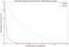 |
Fig. 1 Average nonlinear approximation error as a function of percentage of largest coefficients for 10 000 galaxy images. The solid red line denotes the decay in the starlet space and the blue dashed line denotes the decay in the direct space. |
The starlet transform decomposes an image, x, into a coarse scale, xJ, and wavelet scales, (wj)1 ≤ j ≤ J,  (7)where the first level (j = 1) corresponds to the highest frequencies (i.e. the finest scale). The starlet transform is well suited to most astronomical images, which are generally isotropic. The starlet transformation implemented in this work is that provided in the iSAP1 software package using J = 3 and neglecting the coarse scale.
Minimisation with sparse regularisation is implemented by solving a sequence of problems of the form  (8)where Φ realises the starlet transform without the coarse scale, W(k) is a weighting matrix with 0 ≤ k ≤ kmax, and ⊙ denotes the Hadamard (entrywise) product. Thus, W(k) and Φ(X) are both J ∗ p × n + 1 matrices. k is a reweighting index.
The l1 norm is generally implemented via soft-thresholding (see Eq. (21)). This means that the smallest coefficients will be set to zero and the largest coefficients, which contain the most useful information, will have reduced amplitudes. This can lead to a biased reconstruction of the original signal. Therefore, to alleviate this imbalance and more closely approximate the l0 norm, the reweighting scheme described in Candès et al. (2008) is implemented. Let  denote the solution to Eq. (8) for a given k. The weights are defined by the recurrence relation
  (9)where W(0) denotes the initial weighting matrix. W(0) is set according to the uncertainty that propagates to the estimated galaxies wavelet coefficients in the deconvolution process. The idea is to assign strong weights to the wavelet coefficients that are severely affected by the observational noise and weaker weights to the others. To do so, the wavelet matrix is written as
 ![Mathematical equation: \begin{equation} \boldsymbol{\Phi} = [\mathbf{\Phi}^{1 T},\cdots,\mathbf{\Phi}^{J T}]^T, \label{eq:wav_mat} \end{equation}](/articles/aa/full_html/2017/05/aa29709-16/aa29709-16-eq55.png) (10)where Φjxi is the jth (undecimated) wavelet scale of the image xi.
(10)where Φjxi is the jth (undecimated) wavelet scale of the image xi.
If the PSF convolution matrices, Hi, were invertible and well-conditioned, a straightforward restoration procedure would consist of denoising the vector Hi −1yi by thresholding its wavelet coefficients at the scale j according to a threshold vector tij defined as  (11)for j = 1···J, where σi is the noise standard deviation in the ith galaxy image and κj is a scale dependent tuning parameter, which can be set as 3 or 4 if the noise is Gaussian. If soft-thresholding is used, this amounts to solving the optimisation problem
 ![Mathematical equation: \begin{eqnarray} \begin{aligned} & \underset{\boldsymbol{\alpha}^1,\cdots,\boldsymbol{\alpha}^J}{\text{argmin}} & \frac{1}{2}\|\boldsymbol{\Phi}\mathbf{H}^{i~-1}\vec{y}^{i}-[\boldsymbol{\alpha}^{1 T},\cdots,\boldsymbol{\alpha}^{J T}]^T\|_2^2+ \sum_{j=1}^J \|\vec{t}^{ij}\odot \boldsymbol{\alpha}^j\|_1. \end{aligned} \label{eq:direct_invert} \end{eqnarray}](/articles/aa/full_html/2017/05/aa29709-16/aa29709-16-eq65.png) (12)Such a direct restoration is unsuitable since, as previously mentioned, convolution operators are ill-conditioned, which prevents an accurate inversion. Hi −1, however, can be replaced by HiT, which gives
(12)Such a direct restoration is unsuitable since, as previously mentioned, convolution operators are ill-conditioned, which prevents an accurate inversion. Hi −1, however, can be replaced by HiT, which gives  (13)The initial weighting can thus be defined as
 ![Mathematical equation: \begin{equation} \mathbf{W}^{(0)}_{:,i} = [\vec{t}^{i1 T},\cdots,\vec{t}^{iJ T}]^T, \end{equation}](/articles/aa/full_html/2017/05/aa29709-16/aa29709-16-eq69.png) (14)for i = 0···n.
(14)for i = 0···n.
This weighting allows one to penalise the wavelet coefficients according to the propagated uncertainty. On the other hand, the reweighting scheme decreases the penalty on the wavelet coefficients that are largely above their expected noise level, which mitigates the bias induced by the l1 norm.
Assuming a white Gaussian noise distribution across the whole field-of-view, the noise standard deviation can be estimated as σest = 1.4826 × MAD(Y) where MAD stands for median absolute deviation and  (15)In practice, the number of scales, J, was set to 3, the tuning parameters in Eq. (13) were chosen as κ1 = 3, κ2 = 3, and κ3 = 4, and the number of reweightings was set to 1.
3. Low-rank prior
3.1. Low-rank approximation as a regularisation prior
Solving Eq. (8) is equivalent to deconvolving the detected galaxies independently from one another. A novel way of approaching astronomical image deconvolution is to take advantage of the similarity between galaxy images in a joint restoration process. Indeed, the similar nature of the various galaxy images increases the degeneracy and thus reduces the rank of the matrix X. Therefore, using the prior knowledge that the solution must be of reduced rank can also be used to regularise the inverse problem.
The rank of a matrix can be determined simply by counting the number of non-zero singular values after decomposition (X = UΣVH, H denoting the Hermitian transpose). One may naively assume, then, that the optimisation problem can be regularised by minimising the rank of the reconstruction but, as with the l0 norm in sparse regularisation, this is a non-convex function and is computationally difficult to solve. Consequently, the nuclear norm, 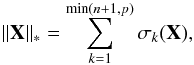 (16)where σk(X) denotes the kth largest singular value of X, is used instead to promote low-rank solutions.
When combined with Eq. (4), this constraint gives the minimisation problem 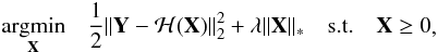 (17)where λ is a regularisation control parameter.
Low-rank techniques have been applied to exoplanet detection by Gomez Gonzalez et al. (2016). Candès & Recht (2009) provide a more complete introduction to low-rank approximations.
3.2. Low-rank implementation
For this work, the assumption is made that a catalogue of similar galaxy images can be approximated by a low-rank representation. Minimisation is implemented via Eq. (17) and the threshold, λ, is calculated as 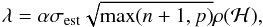 (18)where α is a threshold factor that was set to 1 for this work. The noise estimate, σest, is calculated in the same way as for sparse regularisation.
4. Optimisation
In order to tackle the minimisation problems discussed in the previous sections, a Python code was developed that implements the primal-dual splitting technique described in Condat (2013). Specifically, algorithm 3.1 from Condat (2013) is implemented, neglecting the error terms (as shown in algorithm 1), which aims to solve problems of the form ![Mathematical equation: \begin{eqnarray} \begin{aligned} & \underset{\vec{x}}{\text{argmin}} & [F(\mathbf{X}) + G(\mathbf{X}) + K(\mathcal{L}(\mathbf{X}))] \end{aligned}, \end{eqnarray}](/articles/aa/full_html/2017/05/aa29709-16/aa29709-16-eq86.png) (19)where F is a convex function with gradient ∇F, G and H are functions with proximity operators that can be solved efficiently, and ℒ is a linear operator.
(19)where F is a convex function with gradient ∇F, G and H are functions with proximity operators that can be solved efficiently, and ℒ is a linear operator.
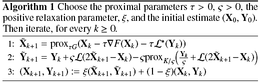
In algorithm 1, X and Y are the primal and dual variables respectively. Upon convergence of the algorithm, the primal variable will correspond to the final solution (i.e. the stack of deconvolved galaxy images).
For all implementations of this algorithm, the primal proximity operator, proxτG, is the positivity constraint and ∇F(X) = ℋ∗(ℋ(X)−Y). ![Mathematical equation: \hbox{$\mathcal{H}^*(\mathbf{Z}) = [\mathbf{H}_0^T\mathbf{Z}_{:,0}, \mathbf{H}_1^T\mathbf{Z}_{:,1}, \dotsc,\mathbf{H}_n^T\mathbf{Z}_{:,n}]$}](/articles/aa/full_html/2017/05/aa29709-16/aa29709-16-eq94.png) .
.
For sparse regularisation, the dual proximity operator, proxK/ς, corresponds to a soft-thresholding with respect to the weights, W(k) in Eq. (8), and the linear operator, ℒ, corresponds to the starlet transform, Φ. Assuming that the matrices Φj in Eq. (10) are circulant, the following inequality holds  (20)For low-rank regularisation, the dual proximity operator, proxK/ς, corresponds to a hard-thresholding of the singular values by the threshold, λ. The linear operator, ℒ, corresponds to the identity operator, In, hence ρ(ℒ) = 1.
The proximal parameters were set to ς = τ = 0.5 and the relaxation parameter was set to ξ = 0.8 for all implementations.
Convergence was obtained when the change in the cost function was less than 0.0001 between iterations.
5. Data
5.1. Galaxy images
The 10 000 galaxy images used for the work presented in this paper were obtained from data provided for the GREAT3 challenge (Mandelbaum et al. 2014)2. Specifically, the single epoch real space-based galaxy images with a constant PSF. GREAT3 was a galaxy shape measurement challenge with the aim of improving the quality of weak gravitational lensing analysis. The challenge used COSMOS data (Koekemoer et al. 2007; Scoville et al. 2007a,b) obtained using the Advanced Camera for Survey (ACS) on the Hubble Space Telescope (HST) and processed with the GalSim software package (Rowe et al. 2015).
Each galaxy image has a pixel scale of 0.05 arcsec, which is twice the resolution of Euclid (0.1 arcsec pixel scale). This resolution was used to avoid the aliasing issues that will have to be taken into account for the real undersampled Euclid images (Cropper et al. 2013). The treatment of these issues is left for future work as the focus of this paper is testing the performance of the deconvolution priors.
Each galaxy is centred within a 96 × 96 pixel postage stamp, but the images were cropped to 41 × 41 to facilitate the use of this data. The pixel flux of the objects range between 0.37 and 814.8, with a median value of 3.7.
These images are well suited to studying Euclid-like observations as the effects of the ACS PSF can be neglected for the purposes of this work, they contain a very small and manageable amount of intrinsic noise, and they are derived from high-resolution space-based data.
5.2. Noise removal
The intrinsic noise is “removed” from each galaxy image, x, by applying soft-thresholding to each image pixel, xi,  (21)where λ = (1−wi) × κ × σest, wi are pixel weights calculated based on local pixel value correlation, κ = 4 and σest is an estimate of the noise.
The noise is estimated by taking the median absolute deviation (MAD) of the starlet transformed image,  (22)
(22)
5.3. Euclid PSFs
The space variant PSFs used are those described in Kuntzer et al. (2016). In total there are 600 unique PSFs corresponding to different positions across the four CCD chips of the Euclid VIS instrument (Cropper et al. 2012). The PSFs were simulated using the VIS pipeline and each one has a resolution 12 times that of Euclid.
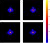 |
Fig. 2 Examples of four space variant Euclid-like PSFs. |
The PSFs are down-sampled by a factor of 6 to match the resolution of the galaxy images. Some examples of the down-sampled Euclid-like PSFs are shown in Fig. 2. These images demonstrate the anisotropy and diversity of the PSFs used.
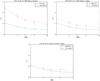 |
Fig. 3 Pixel error as a function of S/N. Mean results from ten random samples of 100 galaxy images with standard deviation error bars (top-left panel). Mean results from ten random samples of 1000 galaxy images with standard deviation error bars (top-right panel). Results for all 10 000 galaxy images (bottom). Solid blue lines indicate results obtained using sparse regularisation and dashed purple lines indicate results obtained using the low-rank approximation. |
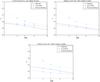 |
Fig. 4 Ellipticity error as a function of S/N. Mean results from ten random samples of 100 galaxy images with standard deviation error bars (top-left panel). Mean results from ten random samples of 1000 galaxy images with standard deviation error bars (top-right panel). Results for all 10 000 galaxy images (bottom). Solid blue lines indicate results obtained using sparse regularisation, dashed purple lines indicate results obtained using the low-rank approximation and dotted green lines indicate results obtained using a pseudo-inverse deconvolution. |
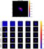 |
Fig. 5 Galaxy 8 of 10 000 reference image (top panel), the image convolved with a Euclid-like PSF and various levels of Gaussian noise added (bottom panel first row), the image after deconvolution with sparse regularisation (bottom panel second row), the residual from sparse deconvolution (bottom panel third row), the image after deconvolution with low-rank regularisation (bottom panel forth row) and the residual from low-rank deconvolution (bottom panel fifth row). Images display the absolute value of the pixels with values less than 0.0005 shown in black. |
5.4. PSF convolution and Gaussian noise
To produce a stack of Euclid-like observations, Y, each image in the stack of cleaned images, X, is normalised such that the pixel values sum to 1.0. It is then convolved with a random Euclid-like PSF (from the sample of 600) and finally Gaussian noise is added. Gaussian additive noise does not encompass all the predicted sources of noise for Euclid VIS images. However, this is a reasonable approximation given that the dominant source of noise expected is readout noise (Cropper et al. 2013).
For this work five values of σ (the noise standard deviation) were chosen such that the observed galaxies have fixed signal-to-noise ratio (S/N) values of 1.0, 2.0, 3.0, 5.0 and 10.0 (i.e. five samples of 10 000 galaxy images each of which has a fixed S/N for every galaxy).
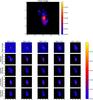 |
Fig. 6 Galaxy 2676 of 10 000 reference image (top panel), the image convolved with a Euclid-like PSF and various levels of Gaussian noise added (bottom panel first row), the image after deconvolution with sparse regularisation (bottom panel second row), the residual from sparse deconvolution (bottom panel third row), the image after deconvolution with low-rank regularisation (bottom panel forth row) and the residual from low-rank deconvolution (bottom panel fifth row). Images display the absolute value of the pixels with values less than 0.0005 shown in black. |
6. Application to data
6.1. Quality metrics
Two metrics are implemented to test the quality of the stack of galaxy images after deconvolution, . The first is the median pixel error, which gives a measure of how similar the deconvolved images are to the original images. The pixel error is given by  (23)A weighted version of the metric is implemented in Appendix A.
The second metric is the median ellipticity error, which gives a measure of how well the galaxy shapes can be estimated from the deconvolved images with respect to the clean images. The ellipticity error is given by  (24)where ε = [ε1,ε2] is a measure of the ellipticity (or shape) of the galaxy image. Details on how the ellipticities were calculated are provided in Appendix B.
The regularisation technique that produces the stack of galaxy images with lower values of Perr and εerr at a given S/N is considered to have the better performance.
6.2. Results
The results of applying the deconvolution code to the data described in Sect. 5 are shown in Figs. 3 and 4. In these figures, solid blue lines indicate results obtained using sparse regularisation and dashed purple lines indicate results obtained using the low-rank approximation. In both figures, the top-left and top-right panels show the mean results with standard deviation error-bars as a function of S/N for ten random samples of 100 and 1000 galaxy images, respectively. The bottom panels show the results as a function of S/N for the full sample of 10 000 galaxy images. Figure 4 contains an additional curve in each panel (green dotted lines) that shows the ellipticities obtained from a pseudo-inverse deconvolution (see Appendix C for details). Techniques similar to this are commonly implemented in weak lensing analyses to measure galaxy ellipticities.
With regards to the pixel error, sparsity appears to produce better results than the low-rank approach. However, the low-rank results improve significantly (by ~10%) as the number of galaxy images increases from 100 to 10 000. When the full sample is used, the difference in the pixel error between the two techniques is approximately 2%.
For the ellipticity error, sparsity performs better when only 100 galaxies are used. With 1000 galaxies, the low-rank results show an improvement of a few percent with respect to sparsity and when all 10 000 are used, low-rank regularisation can provide up to a 10% gain in the ellipticity measurements for low S/N. In all cases, the low-rank method performs better than the pseudo-inverse in terms of ellipticity error.
Figures 5–7 present some examples of individual galaxy images. The top panel in each figure shows the true galaxy images (i.e. the original GREAT3 image after intrinsic noise removal). The first row of the lower panel shows the observed galaxy images (i.e. convolved with Euclid-like PSF) with various levels of Gaussian noise. The second row shows the images after deconvolution with a sparse prior and the third row shows the corresponding residuals ( ). The fourth and fifth rows show the images after deconvolution with a low-rank prior and corresponding residuals respectively. The absolute value of the image pixels are displayed to include negative pixel values and pixels with absolute values below 0.0005 are shown in black for better contrast. In each of these examples both the low-rank and sparsity methods appear to capture the details of the central galaxy pixels. However, there is less structure in the tails of the low-rank residuals.
These results demonstrate the potential benefits of exploiting the low-rank matrix approximation for a large sample of galaxy images where many of the images are similar.
6.3. Convergence speed
The convergence speed is a factor that was not taken into consideration when comparing the performance of the two regularisation techniques. It should be noted, however, that the low-rank method converged more quickly than the sparsity approach as no re-weighting is required.
Reproducible research. In the spirit of reproducible research, the space variant deconvolution code has been made freely available on the CosmoStat website3. The noiseless galaxy images have also been provided along with details on how to repeat the experiments performed in this paper.
7. Conclusions
A sample of 10 000 PSF-free space-based galaxy images were obtained from within the GREAT3 data sets and the intrinsic noise in these images was removed. The images were then convolved with Euclid-like spatially varying PSFs and different levels of Gaussian noise were added to create a series of galaxy images that would be expected from a survey like Euclid.
It has been demonstrated that, using the object oriented deconvolution approach, a new perspective is open for future survey image deconvolution, where images contain many galaxies, which can be assumed to be lying on a given low dimensional manifold. Therefore, a low-rank approximation can be seen as an alternative approach to the most powerful regularising techniques. A deconvolution code that implements both sparsity and a low-rank approximation was developed. This code was applied to various samples of the data and the two regularisation methods were compared by examining the relative pixel and ellipticity errors in the resulting images as a function of S/N.
The results show that for ten random samples of 100 images sparsity outperforms the low-rank approach in terms of the galaxy images recovered and their corresponding shapes. For ten random samples of 1000 images, the low-rank method performs slightly better with regards to shape recovery. When the full sample of 10 000 images is examined, the low-rank method produces significantly lower ellipticity measurement errors, particularly for low S/N where the improvement with respect to sparsity is approximately 10%. Also, the degradation in terms of pixel error compared to sparsity is at most 2%. This implies that for a sufficiently large sample of images, the rank of the matrix can be significantly reduced and used as an effective regularisation prior. This is particularly interesting for projects that require accurate estimates of galaxy shapes.
For future work, it may be interesting to investigate the effects of applying both regularisation techniques simultaneously to see if this can improve the current results. Another interesting study would be to examine the performance when the PSF is not fully known, which is often the case in real galaxy surveys.
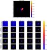 |
Fig. 7 Galaxy 9878 of 10 000 reference image (top panel), the image convolved with a Euclid-like PSF and various levels of Gaussian noise added (bottom panel first row), the image after deconvolution with sparse regularisation (bottom panel second row), the residual from sparse deconvolution (bottom panel third row), the image after deconvolution with low-rank regularisation (bottom panel forth row) and the residual from low-rank deconvolution (bottom panel fifth row). Images display the absolute value of the pixels with values less than 0.0005 shown in black. |
Acknowledgments
This work is supported by the European Community through the grants PHySIS (contract No. 640174) and DEDALE (contract No. 665044) within the H2020 Framework Program of the European Commission. The authors wish to thank Yinghao Ge for initial prototyping of the Python code, and Koryo Okumura, Patrick Hudelot and Jérôme Amiaux for their work on developing the Euclid-like PSFs. The authors additionally acknowledge the Euclid Collaboration, the European Space Agency and the support of the Centre National d’Etudes Spatiales. Finally, the authors wish to thank the anonymous referee for constructive comments that have improved the quality of the work presented.
References
- Bertin, E., & Arnouts, S. 1996, A&AS, 117, 393 [NASA ADS] [CrossRef] [EDP Sciences] [Google Scholar]
- Bobin, J., Sureau, F., Starck, J.-L., Rassat, A., & Paykari, P. 2014, A&A, 563, A105 [NASA ADS] [CrossRef] [EDP Sciences] [Google Scholar]
- Burrows, D. N., Michael, E., Hwang, U., et al. 2000, ApJ, 543, L149 [NASA ADS] [CrossRef] [Google Scholar]
- Candès, E. J., & Recht, B. 2009, Foundations of Computational Mathematics, 9, 717 [CrossRef] [MathSciNet] [Google Scholar]
- Candès, E. J., Wakin, M. B., & Boyd, S. P. 2008, J. Fourier Analysis Applications, 14, 877 [CrossRef] [Google Scholar]
- Condat, L. 2013, J. Optimization Theory Applications, 158, 460 [Google Scholar]
- Cropper, M., Cole, R., James, A., et al. 2012, in Space Telescopes and Instrumentation 2012: Optical, Infrared, and Millimeter Wave, Proc. SPIE, 8442, 84420 [CrossRef] [Google Scholar]
- Cropper, M., Hoekstra, H., Kitching, T., et al. 2013, MNRAS, 431, 3103 [NASA ADS] [CrossRef] [Google Scholar]
- Dixon, D. D., Johnson, W. N., Kurfess, J. D., et al. 1996, A&AS, 120, 683 [NASA ADS] [Google Scholar]
- Garsden, H., Girard, J. N., Starck, J. L., et al. 2015, A&A, 575, A90 [NASA ADS] [CrossRef] [EDP Sciences] [Google Scholar]
- GomezGonzalez, C. A., Absil, O., Absil, P.-A., et al. 2016, A&A, 589, A54 [NASA ADS] [CrossRef] [EDP Sciences] [Google Scholar]
- Gull, S. F., & Daniell, G. J. 1978, Nature, 272, 686 [NASA ADS] [CrossRef] [Google Scholar]
- Hamann, J., Shafieloo, A., & Souradeep, T. 2010, J. Cosmol. Astropart. Phys., 4, 010 [Google Scholar]
- Högbom, J. A. 1974, A&AS, 15, 417 [NASA ADS] [Google Scholar]
- Jorissen, A., Mayor, M., & Udry, S. 2001, A&A, 379, 992 [NASA ADS] [CrossRef] [EDP Sciences] [Google Scholar]
- Kitching, T. D., Miller, L., Heymans, C. E., van Waerbeke, L., & Heavens, A. F. 2008, MNRAS, 390, 149 [NASA ADS] [CrossRef] [Google Scholar]
- Koekemoer, A. M., Aussel, H., Calzetti, D., et al. 2007, ApJS, 172, 196 [NASA ADS] [CrossRef] [Google Scholar]
- Kormendy, J., & Bender, R. 1999, ApJ, 522, 772 [NASA ADS] [CrossRef] [Google Scholar]
- Kuntzer, T., Tewes, M., & Courbin, F. 2016, A&A, 591, A54 [NASA ADS] [CrossRef] [EDP Sciences] [Google Scholar]
- Lanusse, F., Starck, J.-L., Leonard, A., & Pires, S. 2016, A&A, 591, A2 [NASA ADS] [CrossRef] [EDP Sciences] [Google Scholar]
- Leonard, A., Lanusse, F., & Starck, J.-L. 2014, MNRAS, 440, 1281 [NASA ADS] [CrossRef] [Google Scholar]
- Lucy, L. B. 1974, AJ, 79, 745 [NASA ADS] [CrossRef] [Google Scholar]
- Mandelbaum, R., Rowe, B., Bosch, J., et al. 2014, ApJS, 212, 5 [NASA ADS] [CrossRef] [Google Scholar]
- Miley, G. 1980, ARA&A, 18, 165 [Google Scholar]
- Murtagh, F., Starck, J.-L., & Bijaoui, A. 1995, A&AS, 112, 179 [NASA ADS] [Google Scholar]
- Ngolè Mboula, F. M., & Starck, J. 2016, SIAM, submitted [Google Scholar]
- Ngolè Mboula, F. M., Starck, J., Ronayette, S., Okumura, K., & Amiaux, J. 2015, A&A, 575, A86 [NASA ADS] [CrossRef] [EDP Sciences] [Google Scholar]
- Richardson, W. H. 1972, J. Opt. Soc. Amer. (1917–1983), 62, 55 [Google Scholar]
- Rowe, B. T. P., Jarvis, M., Mandelbaum, R., et al. 2015, Astron. Comput., 10, 121 [NASA ADS] [CrossRef] [Google Scholar]
- Scoville, N., Abraham, R. G., Aussel, H., et al. 2007a, ApJS, 172, 38 [NASA ADS] [CrossRef] [Google Scholar]
- Scoville, N., Aussel, H., Brusa, M., et al. 2007b, ApJS, 172, 1 [NASA ADS] [CrossRef] [Google Scholar]
- Starck, J.-L., & Murtagh, F. 1994, A&A, 288, 343 [Google Scholar]
- Starck, J.-L., & Murtagh, F. 1999, Signal Processing, 76, 147 [Google Scholar]
- Starck, J.-L., & Murtagh, F. 2006, Astronomical Image and Data Analysis, 2nd edn. (Springer) [Google Scholar]
- Starck, J.-L., Bijaoui, A., Valtchanov, I., & Murtagh, F. 2000, A&AS, 147, 139 [NASA ADS] [CrossRef] [EDP Sciences] [Google Scholar]
- Starck, J. L., Pantin, E., & Murtagh, F. 2002, PASP, 114, 1051 [NASA ADS] [CrossRef] [Google Scholar]
- Starck, J.-L., Murtagh, F., & Bertero, M. 2015a, in Handbook of Mathematical Methods in Imaging, ed. O. Scherzer (Springer), 2053 [Google Scholar]
- Starck, J.-L., Murtagh, F., & Fadili, J. 2015b, Sparse Image and Signal Processing: Wavelets and Related Geometric Multiscale Analysis (Cambridge University Press) [Google Scholar]
- Sykes, M. V., & Walker, R. G. 1992, Icarus, 95, 180 [NASA ADS] [CrossRef] [Google Scholar]
Appendix A: Weighted pixel error
The pixel errors were additionally calculated using the following metric  (A.1)where w is an isotropic Gaussian kernel with σ = 5. This choice ensures that the central galaxy pixels, which contain most of the information, have higher weights than the tails of the distribution. The results are shown in Fig. A.1.
The relative performance of the two regularisation techniques is consistent with that shown in Fig. 3 and indicates that sparsity better recovers the central pixel values by a few percent.
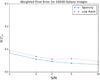 |
Fig. A.1 Weighted pixel error as a function of S/N for all 10 000 galaxy images. Solid blue lines indicate results obtained using sparse regularisation and dashed purple lines indicate results obtained using the low-rank approximation. |
Appendix B: Ellipticity measurement
Ellipticities were measured following the prescription described in Ngolè Mboula & Starck (2016). The ellipticity components are given by 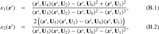 where ⟨ , ⟩ denotes the inner product, Ui are shape projection components
 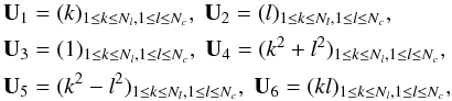 (B.3)and Nc and Nl correspond to the number of columns and lines in the image xi respectively.
It should be noted that Eqs. (B.1) and (B.2) give identical results to more common implementations (e.g. Cropper et al. 2013, Eq. (12)).
Appendix C: Pseudo-inverse deconvolution
The pseudo-inverse deconvolution was implemented as 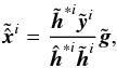 (C.1)where
  ,
,  , and
, and  represent the Fourier transforms of the deconvolved image, the observed image, and the PSF, respectively.
  is the complex conjugate of , and
  is an isotropic Gaussian kernel. For this work a Gaussian kernel with σ = 2 was used.
All Figures
|
Fig. 1 Average nonlinear approximation error as a function of percentage of largest coefficients for 10 000 galaxy images. The solid red line denotes the decay in the starlet space and the blue dashed line denotes the decay in the direct space. |
| In the text | |
|
Fig. 2 Examples of four space variant Euclid-like PSFs. |
| In the text | |
|
Fig. 3 Pixel error as a function of S/N. Mean results from ten random samples of 100 galaxy images with standard deviation error bars (top-left panel). Mean results from ten random samples of 1000 galaxy images with standard deviation error bars (top-right panel). Results for all 10 000 galaxy images (bottom). Solid blue lines indicate results obtained using sparse regularisation and dashed purple lines indicate results obtained using the low-rank approximation. |
| In the text | |
|
Fig. 4 Ellipticity error as a function of S/N. Mean results from ten random samples of 100 galaxy images with standard deviation error bars (top-left panel). Mean results from ten random samples of 1000 galaxy images with standard deviation error bars (top-right panel). Results for all 10 000 galaxy images (bottom). Solid blue lines indicate results obtained using sparse regularisation, dashed purple lines indicate results obtained using the low-rank approximation and dotted green lines indicate results obtained using a pseudo-inverse deconvolution. |
| In the text | |
|
Fig. 5 Galaxy 8 of 10 000 reference image (top panel), the image convolved with a Euclid-like PSF and various levels of Gaussian noise added (bottom panel first row), the image after deconvolution with sparse regularisation (bottom panel second row), the residual from sparse deconvolution (bottom panel third row), the image after deconvolution with low-rank regularisation (bottom panel forth row) and the residual from low-rank deconvolution (bottom panel fifth row). Images display the absolute value of the pixels with values less than 0.0005 shown in black. |
| In the text | |
|
Fig. 6 Galaxy 2676 of 10 000 reference image (top panel), the image convolved with a Euclid-like PSF and various levels of Gaussian noise added (bottom panel first row), the image after deconvolution with sparse regularisation (bottom panel second row), the residual from sparse deconvolution (bottom panel third row), the image after deconvolution with low-rank regularisation (bottom panel forth row) and the residual from low-rank deconvolution (bottom panel fifth row). Images display the absolute value of the pixels with values less than 0.0005 shown in black. |
| In the text | |
|
Fig. 7 Galaxy 9878 of 10 000 reference image (top panel), the image convolved with a Euclid-like PSF and various levels of Gaussian noise added (bottom panel first row), the image after deconvolution with sparse regularisation (bottom panel second row), the residual from sparse deconvolution (bottom panel third row), the image after deconvolution with low-rank regularisation (bottom panel forth row) and the residual from low-rank deconvolution (bottom panel fifth row). Images display the absolute value of the pixels with values less than 0.0005 shown in black. |
| In the text | |
|
Fig. A.1 Weighted pixel error as a function of S/N for all 10 000 galaxy images. Solid blue lines indicate results obtained using sparse regularisation and dashed purple lines indicate results obtained using the low-rank approximation. |
| In the text | |
Current usage metrics show cumulative count of Article Views (full-text article views including HTML views, PDF and ePub downloads, according to the available data) and Abstracts Views on Vision4Press platform.
Data correspond to usage on the plateform after 2015. The current usage metrics is available 48-96 hours after online publication and is updated daily on week days.
Initial download of the metrics may take a while.