© ESO, 2017

1. Introduction

The impact of magnetic fields on the formation of stars and planets is a matter of ongoing discussions (e.g., Matthews & Wilson 2002; Pudritz et al. 2014; Seifried & Walch 2015). For instance, a comprehensive understanding of the relative importance of magnetic fields and turbulence in driving the formation of molecular cores has not been achieved so far (Crutcher et al. 2010a). Magnetic fields are also expected to influence the shape of cloud fragments and the coupling between the gas and dust phase in molecular clouds (Henning et al. 2001).

Direct and indirect measurement methods are available to measure the structure and strength of magnetic fields in star-forming regions. Indirect measurements are performed by observing the polarized emission of elongated dust grains that align with their longer axis perpendicular to the magnetic field lines (e.g., Bertrang et al. 2014; Reissl et al. 2014; Brauer et al. 2016). Based on the dispersions of the polarization direction and the line-of-sight (LOS) velocity, the so-called Chandrasekhar-Fermi method is used to calculate the magnetic field strength in the plane of sky (Chandrasekhar & Fermi 1953). The uncertainty of this method is about ~20% to ~200% and depends on the spatial resolution and how well the velocity dispersion is known (Crutcher 2004; Cho & Yoo 2016). On the other hand, direct measurements are performed by observing spectral lines that are split up by the Zeeman effect (Crutcher 2012). The uncertainty of the magnetic field strength derived from these observations range from ~5% to a few 100% (Crutcher et al. 2010b). With the sensitivity and spectral resolution of currently operating instruments, only the LOS component of the magnetic field strength can be obtained from Zeeman observations (Crutcher et al. 1993). However, the total magnetic field strength can be estimated using a Bayesian analysis (see Crutcher et al. 2010b) or by combining direct and indirect, i.e., complementary measurement methods (Heiles & Haverkorn 2012).

Observations of Zeeman split CN, OH, and HI lines have been used various times in the past to study the magnetic field in molecular clouds (Crutcher & Kazes 1983; Crutcher et al. 1993, 1999; Heiles & Troland 2004; Crutcher et al. 2010b; Crutcher 2012, 2014). From such observations, the magnetic field strength in the LOS direction is usually derived following the approach by Crutcher et al. (1993). However, the limitations and uncertainties of this analysis method have not been well characterized so far. Therefore, we investigate the influence of several physical quantities on the uncertainty of this analysis method. These quantities are the density, temperature, velocity, and magnetic field strength in the molecular cloud.

To achieve this goal, we perform radiative transfer simulations that consider the Zeeman splitting of the 1665 MHz OH line. For this, we use the RT code POLARIS (Reissl et al. 2016) extended by our Zeeman splitting RT extension ZRAD, which is based on the line RT code Mol3D (Ober et al. 2015). With this code, we are able to solve the radiative transfer equation for Zeeman split OH lines via the output of magnetohydrodynamic (MHD) simulations or analytical models.

In this study, we start with a description of the radiative transfer code that we use for our study (Sect. 2). Subsequently, we introduce the mentioned analysis method and the characteristics of the 1665 MHz OH line (Sect. 3). Our results are presented in Sect. 4, where we also describe our approach to investigate the uncertainty of the analysis method. After that, we investigate the influence of the density, temperature, turbulence, and magnetic field strength on the analysis method, which is followed by the impact of variations in the velocity field. In Sect. 5, we discuss how our results can be applied in the case of other transitions of OH and other species. Our conclusions are summarized in Sect. 6.

2. Radiative transfer

For this study, we apply the 3D continuum RT code POLARIS (Reissl et al. 2016). This code solves the RT problem self-consistently on the basis of the Monte Carlo method and allows one to consider magnetic fields as well as various dust grain alignment mechanisms. We extended POLARIS with the capability to consider the RT in spectral lines by implementing the line RT algorithm from the line RT code Mol3D (Ober et al. 2015). In addition, we developed the Zeeman splitting extension ZRAD that takes the Zeeman splitting and polarization of spectral lines into account. The implementation of the Zeeman splitting is based on the works of Landi Degl’Innocenti (1976), Schadee (1978), Rees et al. (1989), and Larsson et al. (2014).

For each considered Zeeman split spectral line, ZRAD requires the following precalculated quantities. Energy levels and transitions taken from the Leiden Atomic and Molecular Database (LAMDA; Schöier et al. 2005), Landé factors of the involved energy levels, line strengths of the allowed transitions between Zeeman sublevels, and radius of the involved gas species.

For the line shape, ZRAD includes natural, collisional, and Doppler broadening mechanisms (line shape: Voigt profile) and the magneto-optic effect (line shape: Faraday-Voigt profile; Larsson et al. 2014). The Voigt and Faraday-Voigt profiles are obtained from the real and imaginary part of the Faddeeva function, respectively (Wells 1999). In ZRAD, a fast and precise solution of the Faddeeva function is realized with the Faddeeva package (Johnson 2012).

3. Model description

3.1. Analysis method

The radiation of Zeeman split spectral lines can be described with the radiative transfer equation in the following form (Larsson et al. 2014): $\begin{array}{ccc}\frac{\mathrm{d}{{I}}_{\mathit{\nu }}}{\mathrm{d}\mathit{s}}& \mathrm{=}& \\ {{K}}_{\mathit{\nu }}& \mathrm{=}& \end{array}$Here, M is the total angular or atomic momentum quantum number projected on the magnetic field vector B. The quantity S₀ is the line strength of the spectral line without Zeeman splitting and S_M′,M′′ are the line strengths of the transitions between Zeeman sublevels. Single prime denotes the upper level; double prime denotes the lower level of the line transition. The quantity n is the gas number density and F(ν′,a) is the Voigt profile line shape function, where $\begin{array}{ccc}{\mathit{\nu }}^{\mathrm{\prime }}& \mathrm{=}& \frac{{\mathit{\nu }}_{\mathrm{0}}\mathrm{+}\mathrm{\Delta }{\mathit{\nu }}_{\mathit{z}}\mathrm{-}\mathit{\nu }}{\mathrm{\Delta }{\mathit{\nu }}_{\mathrm{D}}}\mathit{,}\mathrm{and}\\ \mathit{a}& \mathrm{=}& \frac{\mathit{\gamma }}{\mathrm{4}\mathit{\pi }\mathrm{\Delta }{\mathit{\nu }}_{\mathrm{D}}}\mathrm{·}\end{array}$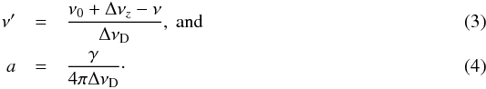Here, ν is the frequency, ν₀ is the frequency of the line peak, Δν_z is the frequency shift due to Zeeman splitting, Δν_D is the Doppler broadening width, and γ is a combination of the natural and collisional broadening width. The calculation of the broadening widths are described in detail by Böttcher (2012).

Only three transitions from M′ to M′′ are allowed. The transitions with ΔM = ± 1 are called σ_±-transitions, whereby the transition with ΔM = 0 is called π-transition. The polarization rotation matrix A_M′,M′′ depends on the type of transition as follows (Landi Degl’Innocenti 1976; Rees et al. 1989; Larsson et al. 2014): 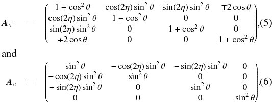$\begin{array}{ccc}{{A}}_{{\mathit{\sigma }}_{\mathrm{\pm }}}& \mathrm{=}& \\ \mathrm{and}& & \\ {{A}}_{\mathit{\pi }}& \mathrm{=}& \end{array}$Here, θ is the angle between the magnetic field B and LOS direction R. The quantity η is the clockwise angle between the vertical polarization direction and the projection of the magnetic field B on the normal plane of the LOS direction R.

By combining Eqs. (1) to (6), we obtain descriptions for the intensity I and circular polarization V similar to the expressions derived by Crutcher et al. (1993) as follows:

$\begin{array}{ccc}& & \mathit{I}\mathrm{=}\mathit{F}\mathrm{(}{\mathit{\nu }}_{\mathrm{0}}\mathrm{+}\mathrm{\Delta }{\mathit{\nu }}_{\mathit{z}}\mathrm{-}\mathit{\nu ,a}\mathrm{)}\mathrm{(}\mathrm{1}\mathrm{+}{\cos }^{\mathrm{2}}\mathit{\theta }\mathrm{)}\mathrm{+}\mathrm{2}\mathit{F}\mathrm{(}{\mathit{\nu }}_{\mathrm{0}}\mathrm{-}\mathit{\nu ,a}\mathrm{)}{\sin }^{\mathrm{2}}\mathit{\theta }\\ & & \mathrm{+}\mathit{F}\mathrm{(}{\mathit{\nu }}_{\mathrm{0}}\mathrm{-}\mathrm{\Delta }{\mathit{\nu }}_{\mathit{z}}\mathrm{-}\mathit{\nu ,a}\mathrm{)}\mathrm{(}\mathrm{1}\mathrm{+}{\cos }^{\mathrm{2}}\mathit{\theta }\mathrm{)}\mathit{,}\\ & & \end{array}$If we assume a line width Δν, which is significantly larger than the Zeeman shift Δν_z, we can derive the circular polarization as follows (see Appendix A for details): $\mathit{V}\mathrm{=}\left(\frac{\mathrm{d}\mathit{I}}{\mathrm{d}\mathit{\nu }}\right)\mathrm{\Delta }{\mathit{\nu }}_{\mathit{z}}\cos \mathit{\theta ,}$(9)whereby the frequency shift Δν_z owing to Zeeman splitting can be calculated with 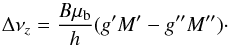$\mathrm{\Delta }{\mathit{\nu }}_{\mathit{z}}\mathrm{=}\frac{\mathit{B}{\mathit{\mu }}_{\mathrm{b}}}{\mathit{h}}\mathrm{(}{\mathit{g}}^{\mathrm{\prime }}{\mathit{M}}^{\mathrm{\prime }}\mathrm{-}{\mathit{g}}^{\mathrm{\prime \prime }}{\mathit{M}}^{\mathrm{\prime \prime }}\mathrm{)}\mathrm{·}$(10)Here, μ_b is the Bohr magneton and g the Landé factor of the corresponding energy level. Following Eqs. (9) and 10, the magnetic field strength in the LOS direction can be obtained by fitting the derivative of the intensity profile to the circular polarization profile of a Zeeman split spectral line. For illustration, Fig. 1 shows this procedure for a spectral line that has a sufficiently low (left) or a Zeeman shift that is too large (right) to estimate the LOS magnetic field strength with Eqs. (9) and (10).

Fig. 1 Schematic illustration of the analysis method to estimate the LOS magnetic field strength. The Zeeman shift is either negligible compared to the spectral line width (left) or on the same order of magnitude (right). In the lower left image, the ratio of dI/ dν to V is proportional to the magnetic field strength in LOS direction Bcosθ. The estimation of the LOS magnetic field strength from the spectral line in the lower right image varies significantly from the present LOS magnetic field strength in the model.

3.2. 1665 MHz transition of OH

In this study, we perform our simulations for the 1665 MHz OH line. In addition, we provide a discussion about the application of our results to observations of other Zeeman split spectral lines in Sect. 5. The Zeeman splitting of the 1665 MHz OH line is caused by the quantized orientation of the total atomic angular momentum on the magnetic field direction. The Landé factors of the energy levels involved in the 1665 MHz OH line can be derived as follows (Radford 1961): $\begin{array}{ccc}{\mathit{g}}_{\mathrm{F}}& \mathrm{=}& {\mathit{g}}_{\mathrm{J}}\frac{\mathit{F}\mathrm{(}\mathit{F}\mathrm{+}\mathrm{1}\mathrm{)}\mathrm{+}\mathit{J}\mathrm{(}\mathit{J}\mathrm{+}\mathrm{1}\mathrm{)}\mathrm{-}\mathit{K}\mathrm{(}\mathit{K}\mathrm{+}\mathrm{1}\mathrm{)}}{\mathrm{2}\mathit{F}\mathrm{(}\mathit{F}\mathrm{+}\mathrm{1}\mathrm{)}}\mathit{,}\\ {\mathit{g}}_{\mathrm{J}}& \mathrm{=}& \frac{\mathrm{1}}{\mathit{J}\mathrm{(}\mathit{J}\mathrm{+}\mathrm{1}\mathrm{)}}\begin{array}{c}\mathrm{⎧}\\ \mathrm{⎪}\\ \mathrm{⎪}\\ \mathrm{⎪}\\ \mathrm{⎪}\\ \mathrm{⎪}\\ \mathrm{⎪}\\ \mathrm{⎨}\\ \mathrm{⎪}\\ \mathrm{⎪}\\ \mathrm{⎪}\\ \mathrm{⎪}\\ \mathrm{⎪}\\ \mathrm{⎪}\\ \mathrm{⎩}\end{array}\frac{\mathrm{3}}{\mathrm{2}}\mathrm{+}\frac{\mathrm{2}\mathrm{(}\mathit{J}\mathrm{-}{\frac{\mathrm{1}}{\mathrm{2}}}^{\mathrm{)}}\mathrm{(}\mathit{J}\mathrm{+}{\frac{\mathrm{3}}{\mathrm{2}}}^{\mathrm{)}}\mathrm{-}\frac{\mathrm{3}}{\mathrm{2}}{\mathit{\lambda }}_{\mathrm{OH}}\mathrm{+}\mathrm{3}}{{\left[\mathrm{4}{\mathrm{(}\mathit{J}\mathrm{+}{\frac{\mathrm{1}}{\mathrm{2}}}^{\mathrm{)}}}^{\mathrm{2}}\mathrm{+}{\mathit{\lambda }}_{\mathrm{OH}}\mathrm{(}{\mathit{\lambda }}_{\mathrm{OH}}\mathrm{-}{\mathrm{4}}^{\mathrm{)}}\right]}^{\frac{\mathrm{1}}{\mathrm{2}}}}\begin{array}{c}\mathrm{⎫}\\ \mathrm{⎪}\\ \mathrm{⎪}\\ \mathrm{⎪}\\ \mathrm{⎪}\\ \mathrm{⎪}\\ \mathrm{⎪}\\ \mathrm{⎬}\\ \mathrm{⎪}\\ \mathrm{⎪}\\ \mathrm{⎪}\\ \mathrm{⎪}\\ \mathrm{⎪}\\ \mathrm{⎪}\\ \mathrm{⎭}\end{array}\mathrm{·}\end{array}$Here, λ_OH is a molecule-specific constant (λ_OH = −7.5). The quantities K, J, and F are the atomic, total orbital, and total atomic angular momentum quantum numbers (1665 MHz OH line: $\mathit{K}\mathrm{=}\frac{\mathrm{1}}{\mathrm{2}}$, $\mathit{J}\mathrm{=}\frac{\mathrm{3}}{\mathrm{2}}$, F = 1). The relative line strengths of transitions between Zeeman sublevels of the 1665 MHz OH line can be calculated as follows (Larsson et al. 2014): $\begin{array}{ccc}\mathrm{\Delta }{\mathit{M}}_{\mathit{F}}& \mathrm{=}& \mathrm{0}\mathrm{:} {\mathit{S}}_{{\mathit{M}}^{\mathrm{\prime }}\mathit{,}{\mathit{M}}^{\mathrm{\prime \prime }}}\mathrm{=}\frac{\mathrm{3}{\mathit{M}}_{\mathit{F}}^{\mathrm{2}}}{\mathit{F}\mathrm{(}\mathit{F}\mathrm{+}\mathrm{1}\mathrm{)}\mathrm{(}\mathrm{2}\mathit{F}\mathrm{+}\mathrm{1}\mathrm{)}}\\ \mathrm{\Delta }{\mathit{M}}_{\mathit{F}}& \mathrm{=}& \mathrm{\pm }\mathrm{1}\mathrm{:} {\mathit{S}}_{{\mathit{M}}^{\mathrm{\prime }}\mathit{,}{\mathit{M}}^{\mathrm{\prime \prime }}}\mathrm{=}\frac{\mathrm{3}\mathrm{(}\mathit{F}\mathrm{\mp }{\mathit{M}}_{\mathit{F}}\mathrm{)}\mathrm{(}\mathit{F}\mathrm{+}\mathrm{1}\mathrm{\pm }{\mathit{M}}_{\mathit{F}}\mathrm{)}}{\mathrm{4}\mathit{F}\mathrm{(}\mathit{F}\mathrm{+}\mathrm{1}\mathrm{)}\mathrm{(}\mathrm{2}\mathit{F}\mathrm{+}\mathrm{1}\mathrm{)}}\mathrm{·}\end{array}$Here, M_F is the total atomic angular momentum quantum number F projected on the magnetic field vector B.

4. Results

4.1. Approach

The analysis method is based on the assumption that the Zeeman shift is small in comparison to the line width. By altering the line shape, several quantities are expected to influence the validity of this assumption. These quantities are the temperature and turbulence (Doppler broadening), density (collisional broadening), and magnetic field strength. We investigate which range of values of these quantities allows a reliable estimation of the LOS magnetic field strength.

Since the gas temperature and turbulence influence the line width in the same way, we use the full width at half maximum (FWHM) of the Doppler broadening line width $\mathrm{\Delta }{\mathit{v}}_{\mathrm{D}}^{\mathit{fwhm}}$ to consider both quantities at once, i.e., $\mathrm{\Delta }{\mathit{v}}_{\mathrm{D}}^{\mathit{fwhm}}\mathrm{=}\mathrm{2}\sqrt{\ln \mathrm{\left(}\mathrm{2}\mathrm{\right)}}\sqrt{\frac{\mathrm{2}{\mathit{N}}_{\mathrm{A}}{\mathit{k}}_{\mathrm{B}}{\mathit{T}}_{\mathrm{OH}}}{{\mathrm{10}}^{-3}{\mathit{m}}_{\mathrm{OH}}}\mathrm{+}{\mathit{v}}_{\mathrm{turb}}^{\mathrm{2}}}\mathit{.}$(15)Here, T_OH is the gas temperature of the OH molecules, m_OH is the molar mass of OH in [g/mol], N_A is the Avogadro constant, k_B is the Boltzmann constant, and v_turb is the turbulent velocity.

For the parameter space, we consider typical conditions in observed molecular clouds (Frerking et al. 1987; Wilson et al. 1997; Minamidani et al. 2008; Crutcher et al. 2010b; Burkhart et al. 2015). These are a hydrogen number density of 9.1 cm^-3 to 1.3 × 10⁷ cm^-3, gas temperature of 10 K to 300 K, turbulent velocity of 100 m/s to 10 km s^-1, and LOS magnetic field strength of 0.1 μG to 3100 μG. Our parameter space (see Table 1) approximately covers these conditions. Each quantity of the parameter space is realized with 128 logarithmically distributed values. We use an abundance of OH/H of 10^-7 that is similar to values used in the works of Crutcher (1979) and Roberts et al. (1995), i.e., OH/H = 4 × 10^-8 and OH/H = 4 × 10^-7, respectively. We consider a spectral resolution of Δv_res = 0.03 km s^-1 that is similar to those of recent observations (Troland & Crutcher 2008; Crutcher et al. 2009, Δv_res = 0.034 km s^-1 and Δv_res = 0.055 km s^-1, respectively).

Our model space is a cube. It is filled with optical thin gas of constant density. The level population of OH is calculated under the assumption of local thermodynamic equilibrium (LTE). However, the choice of the particular method for estimation of the level population is arbitrary, since the analysis method depends only on the ratio of the intensity I to the circular polarization V, but not on the net flux.

To estimate the uncertainty of the analysis method, we compare the LOS magnetic field strength derived by the analysis method B_{LOS, derived} (Eqs. (9), (10); Sect 3.1) with the reference field strength B_LOS. We calculate the reference field strength by averaging the LOS magnetic field strength weighted with the spectral line intensity I along the LOS to the observer as follows: ${\mathit{B}}_{\mathrm{LOS}}\mathrm{=}\frac{{\mathrm{\int }}_{\mathrm{0}}^{\mathrm{obs}}\left({B}\mathrm{\left(}\mathit{s}\mathrm{\right)}\mathrm{·}{{e}}_{\mathrm{LOS}}\right)\mathit{I}\mathrm{\left(}\mathit{s}\mathrm{\right)}\mathrm{d}\mathit{s}}{{\mathrm{\int }}_{\mathrm{0}}^{\mathrm{obs}}\mathit{I}\mathrm{\left(}\mathit{s}\mathrm{\right)}\mathrm{d}\mathit{s}}\mathrm{·}$(16)Here, B(s) is the magnetic field strength, e_LOS is the unit vector in the LOS direction, and s is the path length along the LOS. The relative difference between the derived and the reference LOS magnetic field strength is defined as follows: $\frac{\mathrm{\left|}\mathrm{\Delta }{\mathit{B}}_{\mathrm{LOS}}\mathrm{\right|}}{{\mathit{B}}_{\mathrm{LOS}}}\mathrm{=}\frac{\mathrm{|}{\mathit{B}}_{\mathrm{LOS}\mathit{,}\mathrm{derived}}\mathrm{-}{\mathit{B}}_{\mathrm{LOS}}\mathrm{|}}{{\mathit{B}}_{\mathrm{LOS}}}\mathrm{·}$(17)In this study, we refer to this quantity as the uncertainty of the analysis method and assume that a sufficient reliability is achieved if this uncertainty drops below 10%.

Alternatively, using the same equations, quantities, and assumptions presented in this section and Sect. 3, it is possible to replicate the results of the following section with a simpler approach using multiple Gaussians and comparing the Zeeman shift with the line width. However, the radiative transfer simulations allow us to consider more complex scenarios with variable physical quantities such as density, velocity field, and magnetic field strength (see Sect. 4.3).

4.2. Density, temperature, turbulence, and magnetic field strength

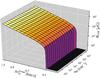Fig. 2 Contour surface where the relative difference between the derived and reference LOS magnetic field strength amounts to 10%. Each parameter combination below the surface corresponds to a lower relative difference.

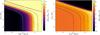Fig. 3 Relative difference between the derived and reference LOS magnetic field strength dependent on the LOS magnetic field strength BLOS and Doppler broadening width $\mathrm{\Delta }{\mathit{v}}_{\mathrm{D}}^{\mathit{fwhm}}$ (hydrogen number density nH = 2 × 105 cm-3). The right image takes the sign of the relative difference into account. The contour lines correspond to relative differences of 1%, 5%, 10%, and 20%.

The contour surface in Fig. 2 shows the LOS magnetic field strength at which the uncertainty of the analysis method is equal to 10% within the considered parameter space. With increasing magnetic field strength, the uncertainty of the analysis method increases. Within typical values of the hydrogen number density, no significant impact of the density on the analysis method can be observed. Therefore, the Doppler effect is the dominant line broadening mechanism in molecular clouds (Δv ≈ Δv_D). The LOS magnetic field strength at which the uncertainty of the analysis method reaches 10% only increases with increasing density if the density is very high (n_H> 10⁷ cm^-3 and thus larger than usually measured in molecular clouds).

Because of the weak dependence of the hydrogen number density on the uncertainty of this method, we now focus our study on the influence of the magnetic field strength and the Doppler broadening owing to temperature and turbulence (see Fig. 3). With increasing line width, the assumption of the analysis method (Δν ≫ Δν_z) is valid even in the case of larger Zeeman shifts, i.e., magnetic field strengths. In addition, spectral lines with a line width of less than ~0.1 km s^-1 always show an uncertainty of more than 10%. Owing to the spectral resolution of Δv_res = 0.03 km s^-1, such lines are too narrow to be resolved sufficiently.

Local minimum. In Fig. 3 (left), a narrow region of minimum relative difference between the derived and reference LOS magnetic field strength can be seen (above the 20% contour line). Here, the analysis method appears to allow one to obtain a very precise LOS magnetic field strength. However, this is not the case. Instead, the assumption of the analysis method is highly violated in this region. For illustration, Fig. 3 (right) shows the relative difference between the derived and reference LOS magnetic field strength with their corresponding sign. In this narrow region, the relative difference changes its sign and, therefore, the uncertainty of the analysis method has to go through a minimum. Below this narrow region, the analysis method overestimates the LOS magnetic field strength and above, the analysis method underestimates the LOS magnetic field strength. As a result, observations of very high LOS magnetic field strengths (> 1 mG) are likely to measure a significantly lower value than present in the cloud, whereby an observed LOS magnetic field strengths of some ~100 μG could be up to ~50% higher.

Magnetic field strength ⊥ LOS. The results shown in Figs. 2 and 3 consider a magnetic field with field vectors only pointing in the LOS direction. An additional magnetic field component perpendicular to the LOS direction adds the π-transition to the intensity profile that changes the superposed line shape (see Eq. (6); Sect. 3.1). In addition, with increasing magnetic field strength perpendicular to the LOS direction, the Zeeman shift Δν_z increases without measuring a higher LOS magnetic field strength. Therefore, we investigate the impact of a magnetic field component perpendicular to the LOS direction on our previous results. For this, we simulate the same cubic model and parameter space as shown in Table 1, but add a magnetic field component perpendicular to the LOS direction with a strength of either 3 or 10 times the LOS component.

As expected, the uncertainty of the analysis method depends on the value of the Zeeman shift Δν_z and therefore on the total magnetic field strength (see Fig. 4). Hence, an upper limit of the total magnetic field strength is necessary to constrain the uncertainty of the analysis method. Crutcher (1999) mentioned that the total magnetic field strength can be estimated by taking two times the mean LOS magnetic field strength. In this case, the impact of a magnetic field component perpendicular to the LOS direction is rather small.

We repeat the simulations shown in Fig. 4 with total magnetic field strengths from 0.5 μG to 100 mG and orientations of the magnetic field vector relative to the LOS from 0° to 89°. By fitting 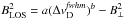${\mathit{B}}_{\mathrm{LOS}}^{\mathrm{2}}\mathrm{=}\mathit{a}\mathrm{(}\mathrm{\Delta }{\mathit{v}}_{\mathrm{D}}^{\mathit{fwhm}}{\mathrm{)}}^{\mathit{b}}\mathrm{-}{\mathit{B}}_{\mathrm{\perp }}^{\mathrm{2}}$ to these results, we obtain an approximation to estimate the maximum LOS magnetic field strength, which can be derived with an uncertainty of less than ~10%, as follows: 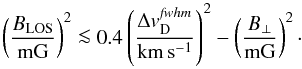${\left(\frac{{\mathit{B}}_{\mathrm{LOS}}}{\mathrm{mG}}\right)}^{\mathrm{2}}\lesssim \mathrm{0.4}{\left(\frac{\mathrm{\Delta }{\mathit{v}}_{\mathrm{D}}^{\mathit{fwhm}}}{\mathrm{km}\hspace{0.17em}{\mathrm{s}}^{-1}}\right)}^{\mathrm{2}}\mathrm{-}{\left(\frac{{\mathit{B}}_{\mathrm{\perp }}}{\mathrm{mG}}\right)}^{\mathrm{2}}\mathrm{·}$(18)Here, B_⊥ is the magnetic field strength perpendicular to the LOS direction and $\mathrm{\Delta }{\mathit{v}}_{\mathrm{D}}^{\mathit{fwhm}}$ is the FWHM Doppler broadening width (see Eq. (15); Sect. 4.1). This equation is applicable only for the Zeeman split 1665 MHz OH line. However, we show in Sect. 5 how this equation can be adapted to other spectral lines as well.

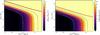Fig. 4 Relative difference between the derived and reference LOS magnetic field strength dependent on the LOS magnetic field strength BLOS and Doppler broadening width $\mathrm{\Delta }{\mathit{v}}_{\mathrm{D}}^{\mathit{fwhm}}$ (hydrogen number density nH = 2 × 105 cm-3). The magnetic field strength perpendicular to the LOS is either 3 (left) or 10 (right) times the LOS magnetic field strength. The contour lines correspond to relative differences of 1%, 5%, 10%, and 20% (left) or 1%, 5%, 10%, and 15% (right).

4.3. Velocity field

In our previous simulations, we neglected the impact of the possible motion of the gas, besides turbulent motion, on the analysis method. However, strong variations in the LOS component of the corresponding velocity field should significantly influence the shape of the spectral lines and, therefore, influence the analysis method. To investigate this, we simulate a Bonnor-Ebert sphere with a constant central density, which can be written as follows (Kaminski et al. 2014): 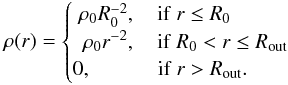$\mathit{\rho }\mathrm{\left(}\mathit{r}\mathrm{\right)}\mathrm{=}\{\begin{array}{c}\\ \\ \\ \end{array}$(19)Here, ρ₀ is a reference density used to achieve a given gas mass, r is the radial distance to the center, and R₀ is a truncation radius that defines the extent of the central region with constant density. We consider a total gas mass of 1 M_⊙ and an outer radius of 1.5 × 10⁴ AU (similar to Bok globule B335; Wolf et al. 2003). The resulting hydrogen number density is in the same range as used in our previous simulations (see Tables 1 and 2). Therefore, the Doppler broadening width determines the line width, which we have chosen to be in agreement with observations (see Table 2; Falgarone et al. 2008). For the velocity field, we assume a collapse with a constant velocity of 1 km s^-1, which is in agreement with velocities found in other studies (Campbell et al. 2016; Wiles et al. 2016). For the magnetic field, we use an approximation found by Crutcher et al. (2010b), which can be written as follows: 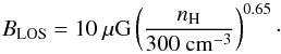${\mathit{B}}_{\mathrm{LOS}}\mathrm{=}\mathrm{10}\mathit{\mu }\mathrm{G}{\left(\frac{{\mathit{n}}_{\mathrm{H}}}{\mathrm{300}\mathrm{c}{\mathrm{m}}^{-3}}\right)}^{\mathrm{0.65}}\mathrm{·}$(20)Here, n_H is the hydrogen number density and the magnetic field is oriented in the LOS direction.

As illustrated in Fig. 5, the uncertainty of the analysis method reaches values larger than 10%. This is caused by the velocity dependent frequency shift of the spectral lines that are related to different magnetic field strengths. If the frequency shift is comparable to the line width, multiple Zeeman split spectral lines are considered in the fitting process. As a consequence, it is not possible to reconstruct the intensity averaged magnetic field strength exactly, if both the gas velocity and magnetic field show significant variations along the LOS. However, this increase of the uncertainty of the analysis method should be small in Zeeman observations of most molecular clouds considering typical velocities on the order of magnitude of ~1 km s^-1.

Fig. 5 Relative difference between the derived and reference LOS magnetic field strength of a spherical model with a Bonnor-Ebert sphere density structure and parameters summarized in Table 2. The image shows the innermost 5000 AU × 5000 AU. The velocity field is chosen to reproduce a collapsing molecular cloud. The contour lines correspond to relative differences of 0.1%, 1%, 3%, and 10%.

5. Zeeman splitting of other spectral lines

In this study, we only consider the 1665 MHz transition of OH. However, by taking particular coefficients into account, our results can be easily applied to other Zeeman split spectral lines as well. For another spectral line i of species j, the Doppler broadening causes a different line width compared to OH due to the different molecular mass of the species (Eqs. (15); Sect. 4.1). The following equation can be used to convert the Doppler broadening width of spectral line i and species j to those used for the 1665 MHz transition of OH in Figs. 2−4 and Eq. (18) (Sect. 4): 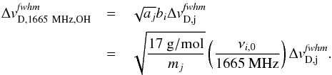$\begin{array}{ccc}\mathrm{\Delta }{\mathit{v}}_{\mathrm{D}\mathit{,}\mathrm{1665}\mathrm{MHz}\mathit{,}\mathrm{OH}}^{\mathit{fwhm}}& \mathrm{=}& \sqrt{{\mathit{a}}_{\mathit{j}}}{\mathit{b}}_{\mathit{i}}\mathrm{\Delta }{\mathit{v}}_{\mathrm{D}\mathit{,}\mathrm{j}}^{\mathit{fwhm}}\\ & \mathrm{=}& \end{array}$(21)Here, m_j is the molar mass of species j and ν_i,0 is the peak frequency of spectral line i. The Doppler broadening acts in units of the velocity and the Zeeman shift in units of the frequency. Therefore, a change in the spectral line peak frequency changes the line width compared to the Zeeman shift. In Eq. (21), this is considered by the coefficient b_i. As a result of this equation, spectral lines with higher peak frequencies and species with a lower mass would provide a larger line width if compared to the Zeeman shift and therefore lower uncertainty of the analysis method. However, with decreasing Zeeman shift compared to the line width, the feasibility to detect the Zeeman effect decreases as well (see Eq. (9)).

For another spectral line i of species j, the Zeeman shift per magnetic field strength Δν_z/B usually differs from the Zeeman shift of OH. By taking this into account, the magnetic field strength can be converted to the field strength used in Figs. 2−4 and Eq. (18) (Sect. 4), i.e.,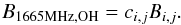${\mathit{B}}_{\mathrm{1665}\mathrm{MHz}\mathit{,}\mathrm{OH}}\mathrm{=}{\mathit{c}}_{\mathit{i,j}}{\mathit{B}}_{\mathit{i,j}}\mathit{.}$(22)Here, c_i,j is the conversion factor of the chosen Zeeman split spectral line i of species j and can be calculated with the following equation (see Eq. (10)): 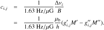$\begin{array}{ccc}{\mathit{c}}_{\mathit{i,j}}& \mathrm{=}& \frac{\mathrm{1}}{\mathrm{1.63}\mathrm{Hz}\mathit{/}\mathit{\mu }\mathrm{G}}\frac{\mathrm{\Delta }{\mathit{\nu }}_{\mathit{z}}}{\mathit{B}}\\ & \mathrm{=}& \end{array}$(23)By combining Eq. (18) from Sect. 4.2 with Eqs. (21) and (22), the maximum LOS magnetic field strength, which can be derived with an uncertainty of less than ~10% can be written as follows: 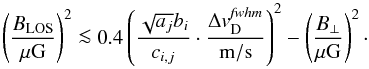${\left(\frac{{\mathit{B}}_{\mathrm{LOS}}}{\mathit{\mu }\mathrm{G}}\right)}^{\mathrm{2}}\lesssim \mathrm{0.4}{\left(\frac{\sqrt{{\mathit{a}}_{\mathit{j}}}{\mathit{b}}_{\mathit{i}}}{{\mathit{c}}_{\mathit{i,j}}}\mathrm{·}\frac{\mathrm{\Delta }{\mathit{v}}_{\mathrm{D}}^{\mathit{fwhm}}}{\mathrm{m}\mathit{/}\mathrm{s}}\right)}^{\mathrm{2}}\mathrm{-}{\left(\frac{{\mathit{B}}_{\mathrm{\perp }}}{\mathit{\mu }\mathrm{G}}\right)}^{\mathrm{2}}\mathrm{·}$(24)In Table 3, we provide an overview of conversion factors for different spectral lines and species that can be used to perform Zeeman observations. We also summarize line widths and magnetic field strengths from observations to estimate if the analysis method provides a negligible uncertainty. It appears that observations of the Zeeman effect in typical molecular clouds are not significantly affected by the uncertainty of the analysis method. Even the spectral lines and species that so far do not provide any observations should be usable up to magnetic field strengths typically observed in molecular clouds.

To check the validity of the conversion factors, we perform simulations with the 99.3 GHz SO line instead of the 1665 MHz OH line (Zeeman splitting parameters from Clark & Johnson 1974; Bel & Leroy 1989; Larsson et al. 2014). We use the same parameters as shown in Table 1 of Sect. 4.2. As expected by the conversion factor in Table 3 and Eq. (24), the maximum LOS magnetic field strength, which can be derived with an uncertainty of less than ~10% shifts by a factor of ~100 to higher field strengths (see Fig. 6).

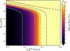Fig. 6 Relative difference between the derived and reference LOS magnetic field strength dependent on the LOS magnetic field strength BLOS and Doppler broadening width $\mathrm{\Delta }{\mathit{v}}_{\mathrm{D}}^{\mathit{fwhm}}$ (hydrogen number density nH = 2 × 105 cm-3). The contour lines correspond to relative differences of 1%, 5%, 10%, and 20%.

6. Conclusions

Observations of Zeeman split spectral lines in star-forming regions, i.e., molecular clouds, represent an established method to study the local magnetic field. We performed simulations with various parameter sets to estimate the value range in which the Zeeman analysis method is applicable for these observations. We found the following results:

• 1.

  Observations of the OH Zeeman effect in typical molecularclouds are not significantly affected by the uncertainty of theanalysis method. However, some observations obtained amagnetic field strength of more than~300 μG, which may result in an uncertainty of the analysis method of > 10%.

• 2.

  Besides OH, multiple species can be used to perform Zeeman observations (CN, HI, other promising species are C₂H, SO, C₂S, C₄H, and CH; Crutcher 2012). We provided equations that allows one to apply our results to other Zeeman split spectral lines of various species as well (Eqs. (21), (22), and (24), Table 3; Sect. 5). We applied these equations to CN and found that observations of the CN Zeeman effect in typical molecular clouds are not significantly affected by the uncertainty of the analysis method.

• 3.

  Within typical values for molecular clouds, the density has almost no impact on the uncertainty of the analysis method, unless it reaches values higher than those typically found in molecular clouds (n_H ≫ 10⁷ cm^-3). As a consequence, the Doppler effect is the dominant broadening mechanism.

• 4.

  The uncertainty of the analysis method increases, if both the gas velocity and magnetic field show significant variations along the LOS. However, this increase should be small in Zeeman observations of most molecular clouds considering typical velocities of ~1 km s^-1.

Acknowledgments

Part of this work was supported by the German Deutsche Forschungsgemeinschaft, DFG project number WO 857/12-1.

References

Appendix A: Derivation of the analysis method

In the following, Eq. (9), which is used to analyze Zeeman split spectral lines, is derived (see Sect. 3.1). The first step is to calculate the derivative of the intensity I with respect to the frequency ν, $\begin{array}{ccc}& & \mathit{I}\mathrm{=}\mathit{F}\mathrm{(}{\mathit{\nu }}_{\mathrm{0}}\mathrm{+}\mathrm{\Delta }{\mathit{\nu }}_{\mathit{z}}\mathrm{-}\mathit{\nu ,a}\mathrm{)}\mathrm{(}\mathrm{1}\mathrm{+}{\cos }^{\mathrm{2}}\mathit{\theta }\mathrm{)}\mathrm{+}\mathrm{2}\mathit{F}\mathrm{(}{\mathit{\nu }}_{\mathrm{0}}\mathrm{-}\mathit{\nu ,a}\mathrm{)}{\sin }^{\mathrm{2}}\mathit{\theta }\\ & & \mathrm{+}\mathit{F}\mathrm{(}{\mathit{\nu }}_{\mathrm{0}}\mathrm{-}\mathrm{\Delta }{\mathit{\nu }}_{\mathit{z}}\mathrm{-}\mathit{\nu ,a}\mathrm{)}\mathrm{(}\mathrm{1}\mathrm{+}{\cos }^{\mathrm{2}}\mathit{\theta }\mathrm{)}\mathit{,}\\ & & \frac{\mathrm{d}\mathit{I}}{\mathrm{d}\mathit{\nu }}\mathrm{=}\frac{\mathrm{d}\mathit{F}\mathrm{(}{\mathit{\nu }}_{\mathrm{0}}\mathrm{+}\mathrm{\Delta }{\mathit{\nu }}_{\mathit{z}}\mathrm{-}\mathit{\nu ,a}\mathrm{)}}{\mathrm{d}\mathit{\nu }}\mathrm{(}\mathrm{1}\mathrm{+}{\cos }^{\mathrm{2}}\mathit{\theta }\mathrm{)}\mathrm{+}\mathrm{2}\frac{\mathrm{d}\mathit{F}\mathrm{(}{\mathit{\nu }}_{\mathrm{0}}\mathrm{-}\mathit{\nu ,a}\mathrm{)}}{\mathrm{d}\mathit{\nu }}{\sin }^{\mathrm{2}}\mathit{\theta }\\ & & \end{array}$If we assume Δν_z → 0, the line function can be written as a Taylor series $\begin{array}{ccc}\mathit{F}\mathrm{(}{\mathit{\nu }}_{\mathrm{0}}\mathrm{+}\mathrm{\Delta }{\mathit{\nu }}_{\mathit{z}}\mathrm{-}\mathit{\nu ,a}\mathrm{)}\mathrm{\approx }\mathit{F}\mathrm{(}{\mathit{\nu }}_{\mathrm{0}}\mathrm{-}\mathit{\nu ,a}\mathrm{)}\mathrm{+}\frac{\mathrm{d}\mathit{F}\mathrm{(}{\mathit{\nu }}_{\mathrm{0}}\mathrm{-}\mathit{\nu ,a}\mathrm{)}}{\mathrm{d}\mathit{\nu }}\mathrm{\Delta }{\mathit{\nu }}_{\mathit{z}}\mathit{,}& & \\ \frac{\mathrm{d}\mathit{F}\mathrm{(}{\mathit{\nu }}_{\mathrm{0}}\mathrm{-}\mathit{\nu ,a}\mathrm{)}}{\mathrm{d}\mathit{\nu }}\mathrm{\Delta }{\mathit{\nu }}_{\mathit{z}}\mathrm{\approx }\mathit{F}\mathrm{(}{\mathit{\nu }}_{\mathrm{0}}\mathrm{+}\mathrm{\Delta }{\mathit{\nu }}_{\mathit{z}}\mathrm{-}\mathit{\nu ,a}\mathrm{)}\mathrm{-}\mathit{F}\mathrm{(}{\mathit{\nu }}_{\mathrm{0}}\mathrm{-}\mathit{\nu ,a}\mathrm{)}\mathit{.}& & \end{array}$

In combination with the following assumptions, we obtain each derivative of the line shape in Eq. (A.2) as follows: 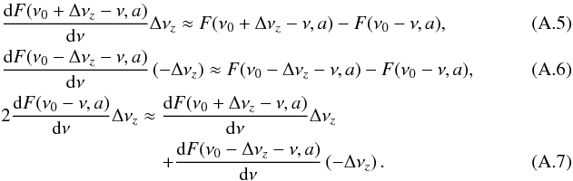$\begin{array}{ccc}& & \\ & & \\ & & \mathrm{2}\frac{\mathrm{d}\mathit{F}\mathrm{(}{\mathit{\nu }}_{\mathrm{0}}\mathrm{-}\mathit{\nu ,a}\mathrm{)}}{\mathrm{d}\mathit{\nu }}\mathrm{\Delta }{\mathit{\nu }}_{\mathit{z}}\mathrm{\approx }\frac{\mathrm{d}\mathit{F}\mathrm{(}{\mathit{\nu }}_{\mathrm{0}}\mathrm{+}\mathrm{\Delta }{\mathit{\nu }}_{\mathit{z}}\mathrm{-}\mathit{\nu ,a}\mathrm{)}}{\mathrm{d}\mathit{\nu }}\mathrm{\Delta }{\mathit{\nu }}_{\mathit{z}}\\ & & \end{array}$Finally, we obtain the equation for the Zeeman analysis (Sect. 3.1, Eq. (9)) using Eqs. (A.5)−(A.7) and multiplying Eq. (A.2) with Δν_zcosθ, $\begin{array}{ccc}\left(\frac{\mathrm{d}\mathit{I}}{\mathrm{d}\mathit{\nu }}\right)\mathrm{\Delta }{\mathit{\nu }}_{\mathit{z}}\cos \mathit{\theta }& \mathrm{=}& \mathrm{2}\mathit{F}\mathrm{(}{\mathit{\nu }}_{\mathrm{0}}\mathrm{+}\mathrm{\Delta }{\mathit{\nu }}_{\mathit{z}}\mathrm{-}\mathit{\nu ,a}\mathrm{)}\cos \mathit{\theta }\\ & & \mathrm{-}\mathrm{2}\mathit{F}\mathrm{(}{\mathit{\nu }}_{\mathrm{0}}\mathrm{-}\mathrm{\Delta }{\mathit{\nu }}_{\mathit{z}}\mathrm{-}\mathit{\nu ,a}\mathrm{)}\cos \mathit{\theta ,}\\ \left(\frac{\mathrm{d}\mathit{I}}{\mathrm{d}\mathit{\nu }}\right)\mathrm{\Delta }{\mathit{\nu }}_{\mathit{z}}\cos \mathit{\theta }& \mathrm{=}\mathit{V}\mathit{.}& \end{array}$

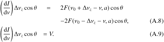
All Tables

All Figures

Fig. 1 Schematic illustration of the analysis method to estimate the LOS magnetic field strength. The Zeeman shift is either negligible compared to the spectral line width (left) or on the same order of magnitude (right). In the lower left image, the ratio of dI/ dν to V is proportional to the magnetic field strength in LOS direction Bcosθ. The estimation of the LOS magnetic field strength from the spectral line in the lower right image varies significantly from the present LOS magnetic field strength in the model.

In the text

	Fig. 2 Contour surface where the relative difference between the derived and reference LOS magnetic field strength amounts to 10%. Each parameter combination below the surface corresponds to a lower relative difference.
In the text

Fig. 3 Relative difference between the derived and reference LOS magnetic field strength dependent on the LOS magnetic field strength BLOS and Doppler broadening width $\mathrm{\Delta }{\mathit{v}}_{\mathrm{D}}^{\mathit{fwhm}}$ (hydrogen number density nH = 2 × 105 cm-3). The right image takes the sign of the relative difference into account. The contour lines correspond to relative differences of 1%, 5%, 10%, and 20%.

In the text

Fig. 4 Relative difference between the derived and reference LOS magnetic field strength dependent on the LOS magnetic field strength BLOS and Doppler broadening width $\mathrm{\Delta }{\mathit{v}}_{\mathrm{D}}^{\mathit{fwhm}}$ (hydrogen number density nH = 2 × 105 cm-3). The magnetic field strength perpendicular to the LOS is either 3 (left) or 10 (right) times the LOS magnetic field strength. The contour lines correspond to relative differences of 1%, 5%, 10%, and 20% (left) or 1%, 5%, 10%, and 15% (right).

In the text

	Fig. 5 Relative difference between the derived and reference LOS magnetic field strength of a spherical model with a Bonnor-Ebert sphere density structure and parameters summarized in Table 2. The image shows the innermost 5000 AU × 5000 AU. The velocity field is chosen to reproduce a collapsing molecular cloud. The contour lines correspond to relative differences of 0.1%, 1%, 3%, and 10%.
In the text

	Fig. 6 Relative difference between the derived and reference LOS magnetic field strength dependent on the LOS magnetic field strength BLOS and Doppler broadening width $\mathrm{\Delta }{\mathit{v}}_{\mathrm{D}}^{\mathit{fwhm}}$ (hydrogen number density nH = 2 × 105 cm-3). The contour lines correspond to relative differences of 1%, 5%, 10%, and 20%.
In the text

References

- Bel, N., & Leroy, B. 1989, A&A, 224, 206 [NASA ADS] [Google Scholar]
- Bertrang, G., Wolf, S., & Das, H. S. 2014, A&A, 565, A94 [NASA ADS] [CrossRef] [EDP Sciences] [Google Scholar]
- Böttcher, M. 2012, Line broadening mechanisms, http://www.phy.ohiou.edu/~mboett/astro401_fall12/broadening.pdf [Google Scholar]
- Brauer, R., Wolf, S., & Reissl, S. 2016, A&A, 588, A129 [NASA ADS] [CrossRef] [EDP Sciences] [Google Scholar]
- Burkhart, B., Collins, D. C., & Lazarian, A. 2015, ApJ, 808, 48 [NASA ADS] [CrossRef] [Google Scholar]
- Campbell, J. L., Friesen, R. K., Martin, P. G., et al. 2016, ApJ, 819, 143 [NASA ADS] [CrossRef] [Google Scholar]
- Chandrasekhar, S., & Fermi, E. 1953, ApJ, 118, 113 [NASA ADS] [CrossRef] [Google Scholar]
- Cho, J., & Yoo, H. 2016, ApJ, 821, 21 [NASA ADS] [CrossRef] [Google Scholar]
- Clark, F. O., & Johnson, D. R. 1974, ApJ, 191, L87 [NASA ADS] [CrossRef] [Google Scholar]
- Crutcher, R. M. 1979, ApJ, 234, 881 [NASA ADS] [CrossRef] [Google Scholar]
- Crutcher, R. M. 1999, ApJ, 520, 706 [NASA ADS] [CrossRef] [Google Scholar]
- Crutcher, R. M. 2004, in The Magnetized Interstellar Medium Proc. Conf., eds. B. Uyaniker, W. Reich, & R. Wielebinski (Copernicus GumbH), 123 [Google Scholar]
- Crutcher, R. M. 2012, ARA&A, 50, 29 [NASA ADS] [CrossRef] [Google Scholar]
- Crutcher, R. 2014, BAAS, 46, 6 [Google Scholar]
- Crutcher, R. M., & Kazes, I. 1983, A&A, 125, L23 [NASA ADS] [Google Scholar]
- Crutcher, R. M., Troland, T. H., Goodman, A. A., et al. 1993, ApJ, 407, 175 [NASA ADS] [CrossRef] [Google Scholar]
- Crutcher, R. M., Troland, T. H., Lazareff, B., Paubert, G., & Kazès, I. 1999, ApJ, 514, L121 [NASA ADS] [CrossRef] [Google Scholar]
- Crutcher, R. M., Hakobian, N., & Troland, T. H. 2009, ApJ, 692, 844 [NASA ADS] [CrossRef] [Google Scholar]
- Crutcher, R. M., Hakobian, N., & Troland, T. H. 2010a, MNRAS, 402, L64 [NASA ADS] [Google Scholar]
- Crutcher, R. M., Wandelt, B., Heiles, C., Falgarone, E., & Troland, T. H. 2010b, ApJ, 725, 466 [NASA ADS] [CrossRef] [Google Scholar]
- Falgarone, E., Troland, T. H., Crutcher, R. M., & Paubert, G. 2008, A&A, 487, 247 [NASA ADS] [CrossRef] [EDP Sciences] [Google Scholar]
- Frerking, M. A., Langer, W. D., & Wilson, R. W. 1987, ApJ, 313, 320 [NASA ADS] [CrossRef] [Google Scholar]
- Heiles, C., & Haverkorn, M. 2012, Space Sci. Rev., 166, 293 [NASA ADS] [CrossRef] [EDP Sciences] [Google Scholar]
- Heiles, C., & Troland, T. H. 2004, ApJS, 151, 271 [NASA ADS] [CrossRef] [Google Scholar]
- Henning, T., Wolf, S., Launhardt, R., & Waters, R. 2001, ApJ, 561, 871 [NASA ADS] [CrossRef] [Google Scholar]
- Hunter, J. D. 2007, Comput. Sci. Engin., 9, 90 [Google Scholar]
- Johnson, S. G. 2012, Faddeeva Package: complex error functions, C++ open-source code [Google Scholar]
- Kaminski, E., Frank, A., Carroll, J., & Myers, P. 2014, ApJ, 790, 70 [NASA ADS] [CrossRef] [Google Scholar]
- Landi Degl’Innocenti, E. 1976, A&AS, 25, 379 [NASA ADS] [Google Scholar]
- Larsson, R., Buehler, S. A., Eriksson, P., & Mendrok, J. 2014, J. Quant. Spectr. Rad. Transf., 133, 445 [Google Scholar]
- Matthews, B. C., & Wilson, C. D. 2002, ApJ, 574, 822 [NASA ADS] [CrossRef] [Google Scholar]
- Minamidani, T., Mizuno, N., Mizuno, Y., et al. 2008, ApJS, 175, 485 [NASA ADS] [CrossRef] [Google Scholar]
- Ober, F., Wolf, S., Uribe, A. L., & Klahr, H. H. 2015, A&A, 579, A105 [NASA ADS] [CrossRef] [EDP Sciences] [Google Scholar]
- Pudritz, R. E., Klassen, M., Kirk, H., Seifried, D., & Banerjee, R. 2014, in Magnetic Fields throughout Stellar Evolution, IAU Symp., 302, 10 [NASA ADS] [Google Scholar]
- Radford, H. E. 1961, Phys. Rev., 122, 114 [NASA ADS] [CrossRef] [Google Scholar]
- Rees, D. E., Durrant, C. J., & Murphy, G. A. 1989, ApJ, 339, 1093 [NASA ADS] [CrossRef] [Google Scholar]
- Reissl, S., Wolf, S., & Seifried, D. 2014, A&A, 566, A65 [NASA ADS] [CrossRef] [EDP Sciences] [Google Scholar]
- Reissl, S., Brauer, R., & Wolf, S. 2016, A&A 593, A87 [NASA ADS] [CrossRef] [EDP Sciences] [Google Scholar]
- Roberts, D. A., Crutcher, R. M., & Troland, T. H. 1995, ApJ, 442, 208 [NASA ADS] [CrossRef] [Google Scholar]
- Schadee, A. 1978, J. Quant. Spectr. Rad. Transf., 19, 517 [Google Scholar]
- Schöier, F. L., van der Tak, F. F. S., van Dishoeck, E. F., & Black, J. H. 2005, A&A, 432, 369 [NASA ADS] [CrossRef] [EDP Sciences] [Google Scholar]
- Seifried, D., & Walch, S. 2015, MNRAS, 452, 2410 [NASA ADS] [CrossRef] [Google Scholar]
- Troland, T. H., & Crutcher, R. M. 2008, ApJ, 680, 457 [NASA ADS] [CrossRef] [Google Scholar]
- Wells, R. J. 1999, J. Quant. Spectr. Rad. Transf., 62, 29 [Google Scholar]
- Wiles, B., Lo, N., Redman, M. P., et al. 2016, MNRAS, 458, 3429 [NASA ADS] [CrossRef] [Google Scholar]
- Wilson, C. D., Walker, C. E., & Thornley, M. D. 1997, ApJ, 483, 210 [NASA ADS] [CrossRef] [Google Scholar]
- Wolf, S., Launhardt, R., & Henning, T. 2003, ApJ, 592, 233 [NASA ADS] [CrossRef] [Google Scholar]