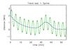
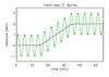
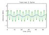
Fig. 4
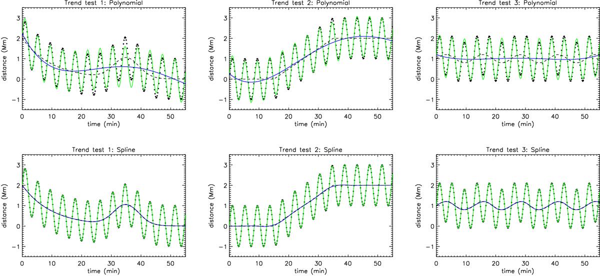
Examples of oscillation fits (green lines) which include a background trend (blue lines) given by a 4th order polynomial (top panels) and our spline procedure (bottom panels) described in Sect. 2.5. The left panels show an example of a localised perturbation in the background (at around 35 min), the middle panels are an example of piecewise linear behaviour, and the right panels show an oscillating background. The spline procedure accurately recovers the actual trend (dashed lines), whereas the low-order polynomial trend can both introduce artifical modulation and fail to account for modulation that is present.
Current usage metrics show cumulative count of Article Views (full-text article views including HTML views, PDF and ePub downloads, according to the available data) and Abstracts Views on Vision4Press platform.
Data correspond to usage on the plateform after 2015. The current usage metrics is available 48-96 hours after online publication and is updated daily on week days.
Initial download of the metrics may take a while.