| Issue |
A&A
Volume 600, April 2017
|
|
|---|---|---|
| Article Number | A7 | |
| Number of page(s) | 11 | |
| Section | Numerical methods and codes | |
| DOI | https://doi.org/10.1051/0004-6361/201628960 | |
| Published online | 20 March 2017 | |
Benchmarking the Multidimensional Stellar Implicit Code MUSIC
1 University of Exeter, Physics and Astronomy, EX4 4QL Exeter, UK
e-mail: This email address is being protected from spambots. You need JavaScript enabled to view it.
2 Université de Lyon, ENS de Lyon, Univ Lyon1, CNRS, Centre de Recherche Astrophysique de Lyon, UMR5574, 69007 Lyon, France
3 Max-Planck-Institut für Astrophysik, Karl Schwarzschild Strasse 1, 85741 Garching, Germany
Received: 18 May 2016
Accepted: 9 September 2016
Abstract
We present the results of a numerical benchmark study for the MUltidimensional Stellar Implicit Code (MUSIC) based on widely applicable two- and three-dimensional compressible hydrodynamics problems relevant to stellar interiors. MUSIC is an implicit large eddy simulation code that uses implicit time integration, implemented as a Jacobian-free Newton Krylov method. A physics based preconditioning technique which can be adjusted to target varying physics is used to improve the performance of the solver. The problems used for this benchmark study include the Rayleigh-Taylor and Kelvin-Helmholtz instabilities, and the decay of the Taylor-Green vortex. Additionally we show a test of hydrostatic equilibrium, in a stellar environment which is dominated by radiative effects. In this setting the flexibility of the preconditioning technique is demonstrated. This work aims to bridge the gap between the hydrodynamic test problems typically used during development of numerical methods and the complex flows of stellar interiors. A series of multidimensional tests were performed and analysed. Each of these test cases was analysed with a simple, scalar diagnostic, with the aim of enabling direct code comparisons. As the tests performed do not have analytic solutions, we verify MUSIC by comparing it to established codes including ATHENA and the PENCIL code. MUSIC is able to both reproduce behaviour from established and widely-used codes as well as results expected from theoretical predictions. This benchmarking study concludes a series of papers describing the development of the MUSIC code and provides confidence in future applications.
Key words: methods: numerical / hydrodynamics / instabilities / stars: evolution
© ESO, 2017
1. Introduction
Despite the inherent three-dimensional nature of stellar interiors the timescales involved in stellar evolution necessitate the use of one-dimensional models. Stellar flows are multidimensional and non-linear in character. Therefore the one-dimensional approach requires parametrisation of three-dimensional effects. Examples of three-dimensional phenomena parametrised into one-dimensional effects are convection, through mixing length theory (Vitense 1953; Böhm-Vitense 1958; Brandenburg 2016), accretion (Siess & Forestini 1996; Siess et al. 1997) and shear driven mixing (Zahn 1992; Maeder & Meynet 1996). With advances in current computing capability the use of multidimensional calculations to calibrate and improve such parametrisations is becoming increasingly feasible. Attempts to improve models of stellar convection have received considerable interest, through the so-called 321D link, Arnett et al. (2015). Recent multidimensional tests of one-dimensional accretion models were carried out by Geroux et al. (2016).
The hydrodynamical processes that influence stellar evolution are non-linear in nature, and not well represented by the idealised test problems available. Many standard test problems for compressible hydrodynamics are supersonic and dominated by shocks, and therefore not representative of the subsonic flows prevalent within stellar interiors. A set of standard tests to compare stellar hydrodynamics codes and evaluate their accuracy has not been clearly defined and organised. Although it is possible to directly characterise and compare such flows through diagnostics such as the convective turnover time, as discussed in Pratt et al. (2016) such flows can vary greatly in space and time, and must be observed over long times to gain meaningful statistics.
In this work we seek to find a middle ground: a set of test problems that are fundamental to stellar interiors but are also simple enough that they may be calculated quickly for the purposes of benchmarking and testing, as well as having well-defined diagnostics, to enable code comparison. We carry out this work primarily to test the accuracy of the numerical methods implemented in the MUltidimensional Stellar Implicit Code, MUSIC.
MUSIC is distinguished from other stellar hydrodynamics codes in that it is both time-implicit and fully compressible. The tests collected in this work have been chosen so that they are useful for comparing a wide variety of physical and numerical models, including codes that are time-explicit and/or those that implement either the anelastic or Boussinesq approximations. The Rayleigh-Taylor, Kelvin-Helmholtz and Taylor-Green tests are relevant to a wide range of hydrodynamical applications. The fourth test, the hydrostatic equilibrium test, is specifically applied to a stellar interior, however the concept could be extended as a general test for the implementation of tabulated equations of state. Additionally the hydrostatic equilibrium test demonstrates for the first time the efficiency of the preconditioning technique applied in MUSIC in a radiatively dominated regime.
Many astrophysical phenomena are known to exhibit dependence on non-ideal effects, such as viscosity. In an effort to minimise non-ideal effects, codes that model such phenomena often do not contain explicit viscous terms. In such a calculation only numerical viscosity acts as a non-ideal term, entering into the solution through the truncation errors of the scheme. A particularly interesting and timely aspect of this work is the examination of the application of such codes to astrophysical phenomena. Within the context of large eddy simulation (LES) calculations this approach is described as the implicit large eddy simulation (ILES) paradigm.
The Rayleigh-Taylor and Kelvin-Helmholtz instabilities are sensitive to non-ideal effects, which only enter into an ILES solution through truncation errors, and vary with resolution. One might ask therefore, to what extent should an ILES code be expected to produce solutions which converge with increasing spatial resolution for these physical problems. For the Rayleigh-Taylor instability we show differences in observed mixing profiles, due to the application of two different ILES methods to a problem sensitive to non-ideal effects. However, a systematic difference between a mixing estimate derived under the assumption of incompressibility, and a more general estimate was observed. For the Kelvin-Helmholtz test we show the velocity field produced in MUSIC calculations exhibits the convergent properties expected from the numerical methods used. The Taylor-Green vortex has been used as a validation test for ILES codes, by monitoring the evolution of the kinetic energy. As this evolution is strongly influenced by truncation errors, we investigate the observed decay of the kinetic energy for different grid-sizes. Additionally we show how the choice of time-step can effect the decay of the kinetic energy.
This paper is structured as follows. In Sect. 2 we give an overview of MUSIC. In Sect. 3 we compare the mixing of a two-dimensional Rayleigh-Taylor instability produced in MUSIC simulations to that produced by ATHENA. In Sect. 4 the ability of MUSIC to reproduce the results for the McNally et al. (2012) Kelvin-Helmholtz instability test problem is investigated. In Sect. 5 the decay of the Taylor-Green vortex is analysed by comparing MUSIC results to previous results from ILES, LES, and DNS calculations. In Sect. 6 we assess the ability of MUSIC to recover hydrostatic equilibrium in a radiatively dominated region of a star. We conclude in Sect. 7, summarising our findings and discussing their implications for future calculations of stellar interiors.
2. The MUSIC code
The MUSIC code is a time-implicit, compressible hydrodynamics code. Initial development is described in Viallet et al. (2011, 2013). Recently, MUSIC has been modified to use the Jacobian-free Newton Krylov (JFNK) method (Viallet et al. 2016). MUSIC solves the Euler equations in the presence of external gravity and thermal diffusion: 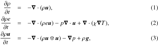 where ρ is the density, e the specific internal energy, u the velocity, p the gas pressure, T the temperature, g the gravitational acceleration, and χ the thermal conductivity. The gravitational acceleration does not change during a MUSIC calculation. It can either be assigned a spatially constant value, or use values calculated consistently with a one-dimensional model which vary with the radial coordinate. In both cases it is implemented as a body force in the momentum equation.
Boundary conditions within MUSIC are implemented using ghost cells. Options include standard techniques, for example reflecting and stress-free, and less common options such as a variety of models for hydrostatic equilibrium as described in Pratt et al. (2016).
Equations (1)–(3) are closed by an equation of state, and an expression for the thermal conductivity. The equation of state within MUSIC can either be taken as an ideal gas equation of state, or a tabulated equation of state, accounting for ionisation and non-ideal effects. The thermal conductivity is given by 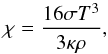 (4)where κ is the Rosseland mean opacity, and σ the Stefan-Boltzmann constant. Equation (4)is the form of the thermal conductivity for photons. For stellar calculations the opacity is interpolated from the OPAL (Iglesias & Rogers 1996) and Ferguson et al. (2005) tables.
The scalar quantities (ρ,e) are defined at cell centres, whereas velocities are located at cell interfaces. To calculate advective fluxes scalar quantities and vector components are extrapolated linearly using an upstream method (Van Leer 1977) and the reconstruction is ensured to be monotonic using the van Leer limiter (Van Leer 1974), resulting in a second-order total variation diminishing (TVD) scheme.
The temporal integration is carried out using the Crank-Nicolson method (Crank & Nicolson 1947), and the resulting non-linear problem is solved using the Newton-Raphson method. At each non-linear iteration a linear problem is solved using the Generalised Minimum Residual (GMRES) method, (Saad & Schultz 1986). A Jacobian-free Newton Krylov approach (for a review see Knoll & Keyes 2004) is used to approximate the matrix-vector products required by GMRES.
The convergence of the GMRES method is improved by using a physics-based preconditioning method, based on the work of Park et al. (2009). Such a preconditioner takes the form of a semi-implicit approximate solution to the full physical system. The preconditioner is semi-implicit in that it treats the stiff terms in the full system implicitly, and the remaining terms explicitly. By adjusting which terms are treated implicitly, the preconditioner can be adapted to a specific problem. Sound waves, and optionally thermal diffusion, are treated implicitly. In this work we present the first application demonstrating the efficiency of the latter case.
2.1. Choice of time-step
The time-step Δt in MUSIC is adaptive and changes throughout the calculation. The time-implicit method used in MUSIC allows large stable time-steps to be taken for the problems considered in this work. The practical choice of the time-step is driven by a desire for an efficient calculation, which also provides an accurate solution. MUSIC will adjust Δt in an attempt to provide a more efficient calculation. This adjustment is restricted by user-provided limits placed on the time-step. The first measure of the time-step used within MUSIC is relative to the hydrodynamical CFL number: 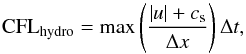 (5)where cs is sound speed, Δt is the time-step, Δx is the grid spacing and u is the flow velocity. A value of CFLhydro = 1 corresponds to the stability limit of a time-explicit scheme. The advective CFL number is defined as,
 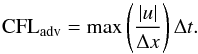 (6)Due to the design of the physics-based preconditioner used in MUSIC, convergence of the linear system becomes poor for values of CFLadv> 0.5 and as such the value of this time-step measure is limited to be at most 0.5 in all calculations in this work.
For calculations involving radiative effects the radiative CFL number is defined:  (7)with χ defined by Eq. (4). Preliminary, low-resolution calculations can be used to determine limiting values for both CFLrad and CFLhydro which provide converged results in as efficient a manner as possible. In cases where multiple constraints are placed on the time-step the most restrictive one is applied.
2.2. Passive scalars
As part of this work, MUSIC has been extended to model a scalar field that is advected with the flow but does not feedback on the dynamics of the fluid. This addition, commonly referred to as “passive scalars” is useful for estimating the mixing and transport of physical quantities such as chemical composition and angular momentum. Example applications of passive scalars may be found in the work of Madarassy & Brandenburg (2010), Falkovich & Fouxon (2005), Schumacher et al. (2005), Brethouwer (2005). The scalars are modelled as compositions, with density equal to the bulk fluid. The conservation equation for a scalar i, with concentration ci is  (8)where ρ is the fluid density, and u the fluid velocity.
MUSIC solves the equation set defined by Eq. (8) using an unpreconditioned Jacobian-free Newton Krylov method. The same discretisation and solver settings as used for the core solver are used for the passive scalar evolution with the exception of the stopping criteria for the non-linear iterations. By default an additional stopping constraint based on the passive scalar evolution is not applied to the non-linear iterations, so that the convergence of the fluid density alone is relied on. This approach is taken to enable the exact replication of results with and without passive scalars supplementing the main equations. We assess the accuracy of the passive scalar implementation in Sect. 3.
This work shall only include cases where two scalars are modelled. For stellar applications the number of species of interest can take a larger value, therefore the implementation within MUSIC was designed to have no restriction on the number of passive scalars. As Eq. (8) evolves mass fractions, there is no guarantee ∑ ici = 1 is maintained. For this work we apply a simple re-normalisation at the end of each time-step, but more sophisticated approaches (e.g. Plewa & Müller 1999) might be required for other problems.
In the applications considered in this work the values of the scalar concentrations do not influence the evolution of the hydrodynamical state defined by Eqs. (1)–(3). For this reason we refer to the scalars as passive. Equation (8) may also be used to describe the evolution of chemical compositions, which do influence the core hydrodynamical state. The solution method for this situation is more complex; the scalar evolution can no longer be decoupled, and instead Eqs. (1)–(3) and (8) must be solved as a single system.
3. Rayleigh-Taylor instability
3.1. Problem description
The Rayleigh-Taylor instability occurs when a dense fluid is accelerated, for example by gravity, into a less dense fluid. This instability occurs in a wide range of astrophysical applications (e.g. Inogamov 1999). The instability has also been the subject of multiple numerical studies (Jun et al. 1995; Dimonte et al. 2004), as well as for code validation, and comparison (e.g. Liska & Wendroff 2003). In this test we assess the ability of MUSIC to model the two-dimensional Rayleigh-Taylor instability. A single mode perturbation was studied, which is provided as a standard example problem1 for the ATHENA code (Gardiner & Stone 2005) and the performance of MUSIC is assessed by comparison to ATHENA2. The problem is similar to that of Liska & Wendroff (2003) except in this work the domain extends to the complete wavelength of the perturbation, so that the entire mushroom is modelled. The problem is calculated on a box defined by −0.25 <x< 0.25 and −0.75 <y< 0.75. The aspect ratio of the box is chosen so that the primary instability remains far from the boundaries for the times considered. A constant gravitational acceleration of magnitude g = 0.1 acts in the negative y-direction. The density is given by,  (9)The pressure is calculated by solving the equation of hydrostatic equilibrium, and is given by
  (10)where P0 = 2.5. The equation of state is an ideal-gas law, with γ = 1.4. The Rayleigh-Taylor instability is sensitive to choices of the initial perturbation (Ramaprabhu et al. 2005). The instability may be seeded by either perturbing the interface, or the velocity. In this work the instability is seeded through the velocity. The velocity perturbation is given by3
![Mathematical equation: \begin{equation} \label{rti_pert} v_y = 0.0025\left[1+\cos\left(4\pi x\right)\right]\left[1+\cos\left(\frac{4}{3} \pi y\right)\right]. \end{equation}](/articles/aa/full_html/2017/04/aa28960-16/aa28960-16-eq37.png) (11)We use dimensionless units, but we note the pressure scale height varies between approximately 25.752 at the bottom of the domain and approximately 11.752 at the top. The linear growth rate of the Rayleigh-Taylor instability depends on the gravitational acceleration, and the dimensionless Atwood number which takes a value of 1/3 in this case. To compare to more realistic values for stellar cases, the scaling implied by the pressure scale height (x0) and the gravitational acceleration (g0) when combined with a scaling for density (ρ0) provide a normalisation for the Euler equations in the presence of external gravitational acceleration, which is the system being described by this test case. Boundary conditions in the vertical directions are calculated by linearly extrapolating the temperature. The density is then calculated according to the equation of hydrostatic equilibrium. Reflective and stress-free boundary conditions are applied to the velocity components. Periodic boundary conditions are applied in the horizontal directions. The evolution of the Rayleigh-Taylor instability, particularly in the non-linear phase is strongly sensitive to non-ideal effects (e.g. viscosity, Cabot & Cook 2006; Lim et al. 2010). MUSIC includes no explicit viscosity, and thus non-ideal effects enter only through errors introduced by the numerical scheme. To aid comparison we run ATHENA without including explicit viscosity. Late time evolution is influenced by secondary Kelvin-Helmholtz instabilities. The break up of the interface between the two fluids through secondary instabilities is strongly dependent on the numerical scheme as discussed by Liska & Wendroff (2003). Comparisons between two codes run without explicit viscosity must be performed with care, because the growth rate of the primary instability, and the development of secondary instabilities are both sensitive to the non-ideal effects caused by the truncation errors of the different numerical schemes.
(11)We use dimensionless units, but we note the pressure scale height varies between approximately 25.752 at the bottom of the domain and approximately 11.752 at the top. The linear growth rate of the Rayleigh-Taylor instability depends on the gravitational acceleration, and the dimensionless Atwood number which takes a value of 1/3 in this case. To compare to more realistic values for stellar cases, the scaling implied by the pressure scale height (x0) and the gravitational acceleration (g0) when combined with a scaling for density (ρ0) provide a normalisation for the Euler equations in the presence of external gravitational acceleration, which is the system being described by this test case. Boundary conditions in the vertical directions are calculated by linearly extrapolating the temperature. The density is then calculated according to the equation of hydrostatic equilibrium. Reflective and stress-free boundary conditions are applied to the velocity components. Periodic boundary conditions are applied in the horizontal directions. The evolution of the Rayleigh-Taylor instability, particularly in the non-linear phase is strongly sensitive to non-ideal effects (e.g. viscosity, Cabot & Cook 2006; Lim et al. 2010). MUSIC includes no explicit viscosity, and thus non-ideal effects enter only through errors introduced by the numerical scheme. To aid comparison we run ATHENA without including explicit viscosity. Late time evolution is influenced by secondary Kelvin-Helmholtz instabilities. The break up of the interface between the two fluids through secondary instabilities is strongly dependent on the numerical scheme as discussed by Liska & Wendroff (2003). Comparisons between two codes run without explicit viscosity must be performed with care, because the growth rate of the primary instability, and the development of secondary instabilities are both sensitive to the non-ideal effects caused by the truncation errors of the different numerical schemes.
3.2. Mixing region width calculation
The mixing in a given simulation was quantified by calculating a mixing region width. By measuring the integrated amount of mixing in a given region such a diagnostic should provide insight into the effect the Rayleigh-Taylor instability could have on a more complex physical system. Mixing of different chemical species through the Rayleigh-Taylor instability could influence stellar structure, convective stability, and nuclear burning rates by altering composition. A mixing width measures the extent to which the two initially separate species have been mixed. This width is calculated by integrating the horizontally averaged mixing fraction, which was calculated using two methods. The first was the method of Cabot & Cook (2006), developed in the incompressible limit. The second method used passive scalars, which capture compressible effects. As discussed in Miczek et al. (2015), Guillard & Viozat (1999), low Mach number flows, which typically occur in stellar interiors, approach the incompressible limit. The Rayleigh-Taylor instability is a subsonic phenomenon. For a grid size of 100 × 300 a maximum Mach number of 0.2607 was obtained with MUSIC, and consequently compressible effects are expected to be small. A comparison between the two methods of estimating mixing should provide insight into the role compressible effects play in mixing in the Rayleigh-Taylor instability.
Following Cabot & Cook (2006), the fraction of dense material in a cell, XH, is  (12)where ρ is the (volume averaged) density of a computational cell, ρH is the initial density of the heavy fluid (2.0 in this work), and ρL is the density of the light fluid (1.0). The fraction of mixed fluid is
  (13)The mixing region width is then defined as
  (14)where ⟨XH⟩ is the average fraction of dense material in a horizontal layer. The Rayleigh-Taylor instability is also analysed using two passive scalar fields, each evolved according to Eq. (8). One passive scalar marks the dense fluid, the other marks the lighter fluid,
  (15)Passive scalars allow the calculation of the mixing region width defined by Eq. (14) without the assumption of incompressibility. In this case the mixing fraction is,
  (16)Having calculated the mixing fraction, the mixing width can once again be calculated using Eq. (14).
As MUSIC is a time-implicit code, the time-step is not restricted by the CFL condition. However, concerns over accuracy and efficiency may provide practical limitations. Given the sensitivity of the Rayleigh-Taylor instability, and to simplify comparison to ATHENA we carry out MUSIC calculations with a fixed value of CFLHydro = 0.8, which is the default value provided for the ATHENA example. This choice does not take advantage of the large time-step allowed by the time-implicit method implemented within MUSIC, it is chosen to simplify comparison with the ATHENA code.
3.3. Effect of grid size
The effect of grid size on the evolution of the Rayleigh-Taylor instability was studied. At early times, the evolution is expected to be dominated by the initial perturbation. Any differences in observed mixing region widths should be attributed to failure to resolve the initial perturbation or changes in non-ideal effects caused by varying the grid size. At later times, secondary instabilities can become more important. Liska & Wendroff (2003) show that less dissipative codes experience a higher rate of secondary instability, and a resulting break-up of the fluid interface.
For this test we use the un-preconditioned JFNK time-integration method in MUSIC to compare with results from the ATHENA code. Identical calculations were carried out using two different two-dimensional grids. Grid sizes of 100 × 300 and 300 × 900 ensured the aspect ratio of the computational cells is equal to 1.0. As the effective viscosity of an ILES calculation depends on the truncation errors of the scheme, differences between results from different codes at a specific grid size should be expected. However, as both MUSIC and ATHENA are spatially second order codes each should experience similar behaviour with increasing grid size. At higher resolution, because non-ideal effects become less significant, secondary instabilities should become more prevalent. The emergence and evolution of secondary instabilities are not seeded by the initial conditions, but through the truncation errors of a given scheme. Therefore as the secondary instabilities grow differences between different schemes may increase.
The evolution of the mixing region width, for MUSIC and ATHENA using the method of Cabot & Cook (2006) is shown in Fig. 1. At early times the Cabot & Cook (2006) mixing region width takes an un-physical negative value in both MUSIC and ATHENA calculations. This is due to the effects of compressibility not being taken into account in this definition of the mixing region width. The high and low grid size calculations with MUSIC diverge around t = 12.0, whereas the two ATHENA calculations show more similar values. That MUSIC results show a stronger dependence on grid size at later times may be indicative of secondary instabilities playing a stronger role in the evolution of the mixing. The influence of secondary instabilities may be enhanced through the non-exact time integration within MUSIC.
Figure 2 shows that calculations from both ATHENA and MUSIC perfectly maintained the symmetry present in the initial conditions. This result demonstrates a physically important feature of the GMRES algorithm: if the matrix vector products respect a given physical symmetry, GMRES is able to produce an approximate solution to the linear problem which is also symmetric. The JFNK method approximates matrix-vector products through the evaluation of the non-linear residual of the full system. In order to obtain a fully symmetric solution, the matrix-vector products must be exactly symmetric. Given the non-associativity of floating point arithmetic, care must be taken in the order of calculations. In this respect codes written in C (or C++), such as ATHENA, have an advantage over codes written in Fortran. The C and C++ standards dictate compilers must respect the order of calculations, whereas Fortran codes are only restricted by order implied by parentheses. Furthermore, not all Fortran compilers (e.g. Intel) follow this restriction by default, as discussed in Corden & Kreitzer (2009).
It is also evident in Fig. 2 that the mixing in the MUSIC calculation becomes asymmetric in the vertical direction; the dense fluid penetrates further into the lighter fluid than the lighter fluid does into the dense fluid. The ATHENA calculation remains more symmetric in this respect. Such enhanced mixing in the lower domain may be caused by the enhanced secondary instabilities discussed previously.
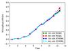 |
Fig. 1 Evolution of mixing region width using the method of Cabot and Cook (2006). |
In contrast to the agreement between the codes in the calculation of the mixing region width Fig. 2 shows significant differences in the development of secondary instabilities. These differences may be caused by differences in the initial conditions, or by differences in the numerical technique applied. The perturbation specified by Eq. (11) is identical in a continuous sense, but the exact discrete form will differ between MUSIC and ATHENA. ATHENA uses co-located variables, whereas MUSIC applies a staggered grid approach. The secondary instabilities which dominate the differences between the two codes are not seeded explicitly by the initial perturbation, and enter into the initial conditions only through discretisation errors. Furthermore truncation errors can seed and enhance secondary instabilities during the course of a simulation. In particular differences between the spatial reconstruction methods used by MUSIC and ATHENA will compound differences between the two results. Given MUSIC and ATHENA obtain similar mixing region widths despite these differences it should be concluded that for the times considered the primary instability dominates mixing.
In addition to verifying the core hydrodynamic method with MUSIC the Rayleigh-Taylor instability was also used to test the implementation of the passive scalars discussed within Sect. 2.2. The impact of not enforcing the non-linear convergence of the passive scalars was assessed by comparing two calculations: firstly a calculation where the passive scalars are not accounted for in the non-linear convergence, and secondly a calculation where we require the corrections to the passive scalars to converge to the same level of accuracy as the primary variables. The measured mixing region width calculated using the volume fractions of the passive scalars was used to compare the two calculations. No assumption of incompressibility is made; the passive scalars act as a dye to measure the amount of mixing within each grid cell. No significant changes in the mixing region width between the two calculations were observed, but enforcing non-linear convergence of the passive scalars the run-time increases by approximately 10%. In all further calculations the convergence of the passive scalars was not explicitly enforced, but such an approach should be assessed for a given application.
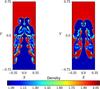 |
Fig. 2 Final density plots for identical Rayleigh-Taylor calculations performed with (left) MUSIC and (right) ATHENA each with a grid size of |

ATHENA can also, optionally, evolve passive scalars. Results obtained using passive scalars in MUSIC were compared to those obtained with ATHENA. The passive scalars evolved by MUSIC and ATHENA also maintain the symmetry of the solution exactly. Figure 3 compares the mixing region widths calculated using passive scalars. In all cases the mixing region width calculated using passive scalars is larger than that observed using the fluid density, suggesting that the assumption of incompressibility systematically underestimates mixing in the case considered here. The un-physical, early time negative mixing region width observed with the Cabot & Cook (2006) method is not observed in the scalar measurements. For both sets of calculations the mixing region width calculated using passive scalars is larger than that using the method of Cabot & Cook (2006) indicating that the assumption of incompressibility systematically underestimates mixing in this case. Furthermore we can conclude that compressible effects are comparable in the calculations of MUSIC and ATHENA.
Two methods of estimating Rayleigh-Taylor induced mixing have been compared using the MUSIC and ATHENA codes. Differences are expected because both codes were used as ILES codes. The MUSIC code appears more sensitive to secondary instabilities. Despite this stronger sensitivity, in both cases a systematic under estimate of mixing is seen when using the method of Cabot & Cook (2006) under the assumption of incompressibility.
4. Kelvin-Helmholtz instability
4.1. Problem description
The Kelvin-Helmholtz instability has been invoked to explain mixing in novae explosions (Casanova et al. 2011) as well as vertical mixing in stellar interiors due to differential rotation (Brüggen & Hillebrandt 2001). Test problems for the instability exist in many forms (Wang et al. 2010; Agertz et al. 2007), here the test case presented by McNally et al. (2012) was used.
McNally et al. (2012) present a set of initial conditions that does not contain sharp discontinuities. Additionally a reference solution, calculated using the PENCIL code (Brandenburg & Dobler 2002; Lyra et al. 2008)4 was provided, in terms of a peak kinetic energy, and the mode amplitude, for a resolution of 40962. The uncertainty in the solution provided was calculated using Richardson extrapolation (Roache 1998, 1994).
 |
Fig. 3 Evolution of mixing region width using passive scalars. |
The mode amplitude and peak kinetic energy were calculated for a series of MUSIC simulations that used different grid sizes (Fig. 4). The peak kinetic energy appears to match the solution of McNally et al. (2012) for grid sizes greater than 5122 while the value obtained for the mode amplitude shows good correspondence with the reference solution for grid sizes greater than 2562. McNally et al. (2012) calculated both the peak kinetic energy and the mode amplitude using a selection of grid based and meshless codes. For the grid based codes, McNally et al. (2012) also showed a smaller error for the mode amplitude compared to that of the peak kinetic energy, at a given grid size.
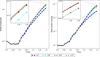 |
Fig. 4 Evolution of the mode amplitude and peak vertical kinetic energy for the Kelvin-Helmholtz instability. The McNally et al. (2012) solution is shown as a black line. Units are dimensionless. |
As in the case of the Rayleigh-Taylor instability, the Kelvin-Helmholtz instability is sensitive to non-ideal effects. In a recent work Lecoanet et al. (2016) considered the possibility of defining an effective Reynolds number for Kelvin-Helmholtz instabilities calculated with differing grid size in the ILES framework. The attribution of an effective Reynolds number was successful for cases without a density contrast. Using the ATHENA code, Lecoanet et al. (2016) were able to find a good match between cases with and without explicit viscosity and attribute this to an approximate increase in Reynolds number with an increase in grid size. The comparison was inconclusive for cases with a density contrast such as the case considered here. For all cases, an increase in grid size corresponds to a decrease in non-ideal effects, but defining an effective Reynolds number is problem dependent, and is not always possible. Care should be taken in interpreting the convergence of such simulations.
4.2. Effect of grid size
In order to assess the convergence of the velocity field for the Kelvin-Helmholtz instability the behaviour of the vertical velocity component with grid size was studied. The spatial discretisation in MUSIC varies between first and second order, due to the application of a gradient limiter. Therefore, for a problem dominated by discontinuities, the convergence of the scheme should be first order, whereas for a smooth solution one should expect the solution to converge at second order.
In the absence of an analytic solution for the velocity field errors with respect to the highest grid size solution we obtained, 40962, were calculated. This does favourably bias the solution produced by MUSIC, in effect it will mask any systematic error in the solution. The presence of a systematic error was ruled out, based on the ability of MUSIC to reproduce the peak kinetic energy and the mode amplitude provided by McNally et al. (2012), and reproduced by several codes in the same study. In the absence of a systematic error, such a study provides an insight and measure of how the error reduces with increasing grid size.
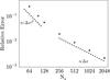 |
Fig. 5 Relative error, as defined by Eq. (17), in the vertical velocity component for the Kelvin-Helmholtz test for different numbers of grid points in the x-direction. In all calculations Ny = Nx. Dashed lines indicate regions where second and first order convergence is observed. |
In order to calculate the relative error at each grid size the largest grid size solution was coarsened to the lower grid size using a volume averaging approach, following the method of Tóth (2000). Such an approach is consistent with the finite volume formulation of MUSIC. Having coarsened the high grid size data the relative absolute value is defined as, 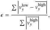 (17)where
  is the low grid size data, and
  is the coarsened high grid size data. Summations are carried out over all grid cells. We plot the variation of this error with grid size in Fig. 5.
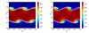 |
Fig. 6 Visualisation of the density in the Kelvin-Helmholtz problem for (left) grid size 642 and (right) grid size 20482 at t = 1.5. |
At low grid sizes the error converges with approximately second order with respect to the grid spacing as expected. As grid size increases (beyond 2562) the convergence tends towards first order. This indicates that the error is dominated by regions in which the solution is discontinuous, causing the spatial scheme to switch to first order. The density at t = 1.5 is shown in Fig. 6 for grid sizes of 642 and 20482. In the 642 case the interface between the layers of different density is smeared across several grid cells, whereas it remains sharper in the 20482 case. By comparing Figs. 6 and 7 it is clear the error is concentrated around the region of the density jump. Such a localisation in error was also shown in Figs. 5 and 6 of McNally et al. (2012).
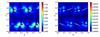 |
Fig. 7 Visualisation of the relative errors for the Kelvin-Helmholtz test compared to the highest grid size 40962 for (left) grid size 642 and (right) grid size 20482 at t = 1.5. |
We have demonstrated the ability of the MUSIC code to reproduce key diagnostics of the Kelvin-Helmholtz instability compared with those reported by McNally et al. (2012). Although MUSIC does not include explicit viscous terms, we have also demonstrated a reduction in error for the velocity field consistent with the numerical methods applied.
5. Decay of the Taylor-Green vortex
5.1. Problem description
The decay of the Taylor-Green vortex (Taylor & Green 1937) has been used as a benchmark for the modelling of turbulent decay in multiple studies. We follow the study of Drikakis et al. (2007; from here on referred to as DFGY2007) which assesses the ability of the monotone implicit large eddy simulation (MILES) method to reproduce features of vortex decay observed when studying the problem with conventional large eddy simulation (LES) and direct numerical simulations (DNS). We do not explicitly attempt to assess the validity of the MILES paradigm, as numerous works on this topic already exist, we simply compare MUSIC to established MILES calculations. This provides an opportunity to investigate the ability of the spatial discretisation in MUSIC to perform as a MILES code. We assess any possible side-effects the time-implicit method has on MILES calculations.
The initial conditions of the Taylor-Green vortex are given by  The domain has an arbitrary uniform density of ρ0 = 1.0. The initial pressure field is
 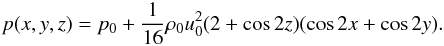 (21)The domain is a cube with edge lengths of 2π, and boundary conditions are periodic in all directions. As in DFGY2007 dimensionless units are used.
In a previous study with MUSIC (Viallet et al. 2016) u0 was fixed to 1.0, and p0 was adjusted to simulate the decay of the Taylor-Green vortex for a range of Mach numbers, 10-1 ≤ Ms ≤ 10-6. However in this work, we adjust p0 so that the initial peak Mach number is Ms = 0.28, as in DFGY2007. Therefore, in addition to verifying MUSIC through comparison to a range of ILES, conventional LES, and DNS simulations, we can also investigate possible compressive effects through comparison to Viallet et al. (2016).
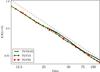 |
Fig. 8 Evolution of the volume averaged, normalised kinetic energy in Taylor-Green vortex simulations. The three simulations shown are identical except for the limitation on the time-step based on the hydrodynamic CFL number. The black dashed line shows a t-2 decay. |
5.2. Effect of time-step
Within ILES calculations the dissipation of kinetic energy occurs through the truncation errors of the scheme. We first investigate the ability of MUSIC to reproduce kinetic energy evolution for different limits on the adaptive time-step. Three calculations, at a grid size of 2563 were carried out. In the first calculation a fixed value of CFLhydro = 0.05 was used (“TGV0.05”). In the remaining two runs, limits were imposed on the hydrodynamical CFL number, defined in Eq. (5), limiting CFLhydro ≤ 10 (“TGV10”), and CFLhydro ≤ 50 (“TGV50”). We show the evolution of the kinetic energy (normalised to its initial value) in Fig. 8. For early times the kinetic energy for all three simulations is very similar.
A decay of t-1.2 of the kinetic energy is predicted by Saffman’s law (Saffman 1967) for homogeneous high Reynolds number turbulence. Skrbek & Stalp (2000) interpret decays faster than t-1.2 as being caused by viscous corrections to the high Reynolds number result. At later times the finite-size of the domain results in a quadratic decay of kinetic energy, as discussed by Lesieur & Ossia (2000). Such a decay has also been observed experimentally by Stalp et al. (1999).
We fit power-law decays for the kinetic energy in MUSIC calculations for two time periods. The first spans to 8.4 ≤ t ≤ 10. This covers the time from the peak dissipation rate shown in Fig. 9, and the point at which the decay takes on a steady, steeper decay. Power-law decays are also fit for the period t> 10. Both sets of values are recorded in Table 1. For the fits to the early (8.4 ≤ t ≤ 10) time we find a values between the high and low Reynolds number predictions from Saffman’s law, indicating the calculations are in neither extreme regime.
All calculations show similar evolution, up until t = 20, at which point the calculation with the least restrictive time-step constraints (TGV50) shows a slightly increased rate of dissipation. The TGV10 case matches the fixed time-step calculation until approximately t = 25 at which point it too shows a slight increase in dissipation rate when compared to the fixed CFL number calculation. At later times the TGV50 and TGV10 calculations show similar kinetic energy, both slightly less than the fixed CFL number calculation. All three data sets show decays slightly slower than t-2. These results can be compared to Fig. 5 of DFGY2007. This shows four ILES and three LES schemes producing an approximate decay of kinetic energy as t-2. All schemes shown in DFGY2007 show fluctuations around the t-2 decay, indeed the differences seen in the three sets of calculations using MUSIC appear smaller than those observed between different ILES schemes in DFGY2007.
5.3. Effect of grid size
The effect of grid size on the decay of the Taylor-Green vortex until t = 20 was investigated using a series of calculations at grid sizes of 643, 1283, 2563 and 5123. These calculations were limited so that CFLhydro ≤ 10. This choice of time-step restriction is chosen so that the kinetic energy is converged with respect to the time-step, and results in a shorter run-time than the other choices considered. We explicitly calculate the rate of change of kinetic energy density ( )for each grid size at each time-step.
Power law decay constants fitted to the observed kinetic energy from 2563 Taylor-Green vortex calculations.
We first compare the 643 calculation shown in Fig. 9 with those shown in Fig. 4 of Viallet et al. (2016). Viallet et al. (2016) show that MUSIC is able to produce consistent results for a range of Mach numbers, 10-1 ≤ Ms ≤ 10-6. However results presented here show fluctuations around the profile presented in Viallet et al. (2016). As these fluctuations only manifest in MUSIC simulations with Ms> 10-1 they are likely a result of acoustic fluctuations. Similar fluctuations are also present in Fig. 2e of DFGY2007. They are not present in the incompressible conventional LES calculations presented in DFGY2007.
 |
Fig. 9 Decay rate of the Taylor-Green vortex, for different grid sizes. |
In ILES calculations non-ideal effects should become less influential with increased grid size. Therefore as the grid size is increased in ILES calculations the solution should tend towards higher Reynolds number results from conventional DNS calculations. We initially compare the evolution of kinetic energy from MUSIC with Fig. 2a of DFGY2007, which shows results from the DNS calculations of Brachet et al. (1983). The peak dissipation is observed around t = 9 for all MUSIC calculations. This is also seen in all DNS calculations shown in DFGY2007, except the lowest Reynolds number, Re = 400, which shows a broad peak, from around t = 6 to t = 9. Such a period of high dissipation is also observed in the lowest grid size MUSIC simulation 643, albeit with an additional peak at approximately t = 9.
Two general patterns of behaviour can be observed with increasing grid size in Fig. 9. Firstly, the initial high rate of dissipation around t = 5 quickly reduces with increasing grid size. This is observed both in the DNS calculations of Brachet et al. (1983), as well as in the MILES calculations shown in Fig. 2e of DFGY2007. Additionally, the maximum dissipation observed at t = 9 increases with increasing grid size. A similar pattern is seen with increasing Reynolds number for DNS calculations. The peak value of dissipation in the 5123 MUSIC calculations appears comparable to that observed in DNS calculations with Reynolds numbers of 3000 and 5000.
Finally we note the double peak feature in the dissipation rate, seen for both 1283 and 2563 grid sizes in MUSIC calculations. Such a double peak is also apparent in the 1283 MILES calculations of Fig. 3 in DFGY2007 (calculated using the TURMOIL3D code, Youngs 1991), but not other MILES calculations. DFGY2007 suggest that such a double peak feature could be produced by more dispersive numerical schemes. However, DFGY2007 do not show whether this peak is present in other calculations using TURMOIL3D, so further comparison is not possible.
We have demonstrated not only the capability of MUSIC to reproduce features of the decay of the Taylor-Green vortex seen in other ILES calculations, but also that an increase in grid size reproduces the same qualitative changes in dissipation seen in DNS calculations of increasing grid size. We stress that this work is not in itself a verification of the ILES paradigm. We do show that whilst an increase in the computational time-step does result in fluctuations of the observed kinetic energy, the range of these fluctuations is within the range observed for differing ILES schemes.
6. Hydrostatic equilibrium under realistic stellar conditions
A final test based on hydrostatic equilibrium under realistic stellar conditions was performed. The MUSIC code is primarily devoted to studying fluid processes in stellar interiors on timescales where hydrostatic equilibrium prevails. It is thus crucial to verify the ability of the code to converge towards a state of hydrostatic equilibrium in a multidimensional configuration. As MUSIC uses a staggered grid, a balance between the pressure gradient and the gravitational forces should be obtainable without resorting to more specialised methods, for example a well-balanced technique (e.g. Käppeli & Mishra 2016) as used in codes with co-located variables.
The stellar model selected for this test is a 20 M⊙ Main Sequence star with zero metallicity calculated with the Lyon one-dimensional (1D) stellar evolution code (Baraffe & El Eid 1991; Baraffe et al. 1998). The 1D model used as an initial setup for the present test is characterised by a surface luminosity L ~ 1.9 × 1038 erg s-1( ~ 5 × 10⁴L⊙), radius R ~ 1.9 R⊙ and effective temperature Teff ~ 6.2 × 10⁴ K. It is in thermal equilibrium, meaning that the nuclear energy production in the central regions counterbalances the energy loss at the surface. We chose this model because of its simple interior structure, with a convective core and a radiative envelope. Due to the absence of metals in the envelope this model exhibits low radiative opacities in the outer layers. Consequently convection is not able to develop close to the stellar surface, and we are able to choose a fully radiative portion of the stellar envelope for our numerical domain.
The test was performed in two-dimensional spherical geometry (with azimuthal symmetry) that considers only a small portion of the radiative envelope. In order to obtain rapid convergence whilst using large CFL numbers, we avoid the region very close to the surface characterised by steep temperature and density gradients (see Fig. 10). We use a grid size of 120 × 120. The radial grid has a fixed radial spacing and is defined between 0.96 R and 0.99 R. In the angular direction, the grid covers the region 50° ≤ θ ≤ 55°.
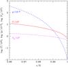 |
Fig. 10 Radial profiles from the 1D model of the temperature (in units of 105 K), density (in units of 10-6 g cm-3) and sound speed (in units of 107 cm s-1) in the outer radiative envelope of a 20 M⊙ star with zero metallicity. R is the total stellar radius. |
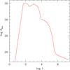 |
Fig. 11 Evolution of the total kinetic energy Ekin (in erg) during the relaxation process toward hydrostatic equilibrium in the stellar model. Time t is in seconds. |
Periodic boundary conditions in the angular direction are used. The boundary conditions at the radial extent of the domain are reflective for the radial velocity component, and stress-free for the tangential component. The inner and outer radial boundary conditions on the energy flux assume the constant luminosity given by the 1D initial model. The inner and outer radial boundary conditions for the density are based on the assumption of hydrostatic equilibrium (see Eq. (5) of Pratt et al. 2016). Pratt et al. (2016) tested various boundary conditions and this set provides the best convergence toward hydrostatic equilibrium measured by the maximum velocity magnitude obtained at the end of the simulation.
The model requires some time to relax toward very low velocity magnitudes that characterise the state of hydrostatic equilibrium. This is illustrated in Fig. 11 by the evolution of the total kinetic energy contained in the numerical domain. After 106 s, the highest velocity magnitude within the domain remains around ~ 7 × 10⁻⁵ cm s-1. This low velocity corresponds to a Mach number of ~ 10-11. The minimum value for the velocity magnitude is around ~ 8 × 10⁻¹⁰ cm s-1.
The most severe constraint on the timestep during the relaxation process is imposed by the radiative CFL number, defined by Eq. (7). This stems from the combination of high temperature, low density and low opacity in the stellar model, resulting in very high radiative diffusivity Drad ≡ χ/ (ρcP) ∝ T3/ (κρ2), with cP the specific heat at constant pressure and the other quantities defined in Eq. (4). We limit the radiative CFL number to 500 to reduce the number of non-linear iterations and to obtain the best performance of our solver. The preconditioner within MUSIC is designed to target the physics which is restricting convergence. Due to the level of thermal diffusion in this problem it is necessary to apply the form of the physics based preconditioner which treats thermal diffusion implicitly. Without targeting the thermal diffusion with the preconditioner, the convergence of the linear system fails. The large time-step facilitated by the application of this preconditioner allows the structure to settle towards equilibrium efficiently, without the need of explicit damping. We have not tried to fine-tune the parameters of our solver (see Viallet et al. 2016) to reach lower velocities. We consider these results and the convergence toward a hydrostatic equilibrium state as satisfactory given the extremely low Mach numbers reached at the end of the relaxation process.
7. Conclusion
This work builds on previous descriptions of the MUSIC code by providing a series of non-linear, multidimensional tests. In a model of the Rayleigh-Taylor instability MUSIC produces comparable mixing layer widths to the well established ATHENA code. The test was additionally used to assess the new implementation of passive scalars within MUSIC. The Kelvin-Helmholtz test of McNally et al. (2012) provides reference solutions for peak kinetic energy, and the mode amplitude, which are both reproducible using the MUSIC code. Furthermore the variable nature of the convergence of the velocity field for this test problem is examined. Like many other astrophysical codes MUSIC does not include explicit viscous terms. Using the Taylor-Green vortex the ability of MUSIC to reproduce features of established ILES codes, and conventional LES codes is shown, as well as observations suggesting an increasing effective Reynolds number with increasing grid size. Finally, MUSIC converges towards the hydrostatic equilibrium within a radiatively dominated portion of a star, in an efficient manner through the application of a preconditioning technique adapted to such a problem.
Whilst this work aims to increase confidence in MUSIC calculations, we intend it to be of general use as the basis of a code comparison test suite for hydrodynamics. Such a benchmarking exercise provides confidence and credibility to simulations. This work concludes the development of the hydrodynamical core of MUSIC. Future work will focus on applications to stellar interiors, such as convective overshooting and shear-driven mixing.
We use ATHENA version 4.2 available from https://trac.princeton.edu/Athena/wiki/AthenaDocsDownLd
Equation (11) is taken from the ATHENA source code.
Available from http://pencil-code.nordita.org/
Acknowledgments
This project has received funding from the European Unions Seventh Framework Programme for research, technological development and demonstration under grant agreement No. 320478. The calculations for this paper were performed on the DiRAC Complexity machine, jointly funded by STFC and the Large Facilities Capital Fund of BIS, and the University of Exeter Super- computer, a DiRAC Facility jointly funded by STFC, the Large Facilities Capital Fund of BIS and the University of Exeter. We are very thankful to Colin McNally for providing his results for the Kelvin-Helmholtz test.
References
- Agertz, O., Moore, B., Stadel, J., et al. 2007, MNRAS, 380, 963 [NASA ADS] [CrossRef] [Google Scholar]
- Arnett, W. D., Meakin, C., Viallet, M., et al. 2015, ApJ, 809, 30 [NASA ADS] [CrossRef] [Google Scholar]
- Baraffe, I., & El Eid, M. F. 1991, A&A, 245, 548 [NASA ADS] [Google Scholar]
- Baraffe, I., Chabrier, G., Allard, F., & Hauschildt, P. H. 1998, A&A, 337, 403 [NASA ADS] [Google Scholar]
- Böhm-Vitense, E. 1958, Z. Astrophys., 46, 108 [Google Scholar]
- Brachet, M. E., Meiron, D. I., Orszag, S. A., et al. 1983, J. Fluid Mech., 130, 411 [NASA ADS] [CrossRef] [Google Scholar]
- Brandenburg, A. 2016, ApJ, 832, 6 [Google Scholar]
- Brandenburg, A., & Dobler, W. 2002, Comput. Phys. Commun., 147, 471 [NASA ADS] [CrossRef] [Google Scholar]
- Brethouwer, G. 2005, J. Fluid Mech., 542, 305 [NASA ADS] [CrossRef] [Google Scholar]
- Brüggen, M., & Hillebrandt, W. 2001, MNRAS, 320, 73 [NASA ADS] [CrossRef] [Google Scholar]
- Cabot, W. H., & Cook, A. W. 2006, Nat. Phys., 2, 562 [CrossRef] [Google Scholar]
- Casanova, J., José, J., García-Berro, E., Shore, S. N., & Calder, A. C. 2011, Nature, 478, 490 [NASA ADS] [CrossRef] [PubMed] [Google Scholar]
- Corden, M. J., & Kreitzer, D. 2009, Consistency of floating-point results using the intel compiler or why doesn’t my application always give the same answer, Tech. rep., Technical report, Intel Corporation, Software Solutions Group [Google Scholar]
- Crank, J., & Nicolson, P. 1947, in Proc. Cambridge Phil. Soc., 43, 50 [Google Scholar]
- Dimonte, G., Youngs, D., Dimits, A., et al. 2004, Phys. Fluids (1994-present), 16, 1668 [Google Scholar]
- Drikakis, D., Fureby, C., Grinstein, F. F., & Youngs, D. 2007, Journal of Turbulence, 8 [Google Scholar]
- Falkovich, G., & Fouxon, A. 2005, Phys. Rev. Lett., 94, 214502 [NASA ADS] [CrossRef] [Google Scholar]
- Ferguson, J. W., Alexander, D. R., Allard, F., et al. 2005, ApJ, 623, 585 [NASA ADS] [CrossRef] [Google Scholar]
- Gardiner, T. A., & Stone, J. M. 2005, J. Comput. Phys., 205, 509 [Google Scholar]
- Geroux, C., Baraffe, I., Viallet, M., et al. 2016, A&A, 588, A85 [NASA ADS] [CrossRef] [EDP Sciences] [Google Scholar]
- Guillard, H., & Viozat, C. 1999, Comp. and Fluids, 28, 63 [Google Scholar]
- Iglesias, C. A., & Rogers, F. J. 1996, ApJ, 464, 943 [NASA ADS] [CrossRef] [Google Scholar]
- Inogamov, N. 1999, Astrophys. Space Phys. Rev., 10, 1 [Google Scholar]
- Jun, B.-I., Norman, M. L., & Stone, J. M. 1995, ApJ, 453, 332 [NASA ADS] [CrossRef] [Google Scholar]
- Käppeli, R., & Mishra, S. 2016, A&A, 587, A94 [NASA ADS] [CrossRef] [EDP Sciences] [Google Scholar]
- Knoll, D. A., & Keyes, D. E. 2004, J. Comput. Phys., 193, 357 [NASA ADS] [CrossRef] [Google Scholar]
- Lecoanet, D., McCourt, M., Quataert, E., et al. 2016, MNRAS, 455, 4274 [NASA ADS] [CrossRef] [Google Scholar]
- Lesieur, M., & Ossia, S. 2000, Journal of Turbulence, 1, 007 [NASA ADS] [CrossRef] [Google Scholar]
- Lim, H., Iwerks, J., Glimm, J., & Sharp, D. H. 2010, Proc. Nat. Acad. Sci., 107, 12786 [NASA ADS] [CrossRef] [Google Scholar]
- Liska, R., & Wendroff, B. 2003, SIAM Journal on Scientific Computing, 25, 995 [CrossRef] [Google Scholar]
- Lyra, W., Johansen, A., Klahr, H., & Piskunov, N. 2008, A&A, 479, 883 [NASA ADS] [CrossRef] [EDP Sciences] [Google Scholar]
- Madarassy, E. J., & Brandenburg, A. 2010, Phys. Rev. E, 82, 016304 [NASA ADS] [CrossRef] [Google Scholar]
- Maeder, A., & Meynet, G. 1996, A&A, 313, 140 [NASA ADS] [Google Scholar]
- McNally, C. P., Lyra, W., & Passy, J.-C. 2012, ApJS, 201, 18 [NASA ADS] [CrossRef] [Google Scholar]
- Miczek, F., Röpke, F., & Edelmann, P. 2015, A&A, 576, A50 [NASA ADS] [CrossRef] [EDP Sciences] [Google Scholar]
- Park, H., Nourgaliev, R. R., Martineau, R. C., & Knoll, D. A. 2009, J. Comput. Phys., 228, 9131 [NASA ADS] [CrossRef] [Google Scholar]
- Plewa, T., & Müller, E. 1999, A&A, 342, 179 [NASA ADS] [Google Scholar]
- Pratt, J., Baraffe, I., Goffrey, T., et al. 2016, A&A, 593, A121 [NASA ADS] [CrossRef] [EDP Sciences] [Google Scholar]
- Ramaprabhu, P., Dimonte, G., & Andrews, M. 2005, J. Fluid Mech., 536, 285 [NASA ADS] [CrossRef] [Google Scholar]
- Roache, P. J. 1994, J. Fluids Eng. 116, 405 [Google Scholar]
- Roache, P. J. 1998, Verification and validation in computational science and engineering (Hermosa) [Google Scholar]
- Saad, Y., & Schultz, M. H. 1986, SIAM Journal on scientific and statistical computing, 7, 856 [Google Scholar]
- Saffman, P. 1967, Phys. Fluids (1958–1988), 10, 1349 [NASA ADS] [CrossRef] [Google Scholar]
- Schumacher, J., Sreenivasan, K. R., & Yeung, P. 2005, J. Fluid Mech., 531, 113 [NASA ADS] [CrossRef] [Google Scholar]
- Siess, L., & Forestini, M. 1996, A&A, 308, 472 [NASA ADS] [Google Scholar]
- Siess, L., Forestini, M., & Bertout, C. 1997, A&A, 326, 1001 [NASA ADS] [Google Scholar]
- Skrbek, L., & Stalp, S. R. 2000, Phys. Fluids, 12, 1997 [NASA ADS] [CrossRef] [Google Scholar]
- Stalp, S. R., Skrbek, L., & Donnelly, R. J. 1999, Phys. Rev. Lett., 82, 4831 [NASA ADS] [CrossRef] [Google Scholar]
- Taylor, G., & Green, A. 1937, Math. Phys. Sci., Proc. Roy. Soc. London Ser. A, 158, 499 [Google Scholar]
- Tóth, G. 2000, J. Comput. Phys., 161, 605 [Google Scholar]
- Van Leer, B. 1974, J. Comput. Phys., 14, 361 [NASA ADS] [CrossRef] [Google Scholar]
- Van Leer, B. 1977, J. Comput. Phys., 23, 276 [Google Scholar]
- Viallet, M., Baraffe, I., & Walder, R. 2011, A&A, 531, A86 [NASA ADS] [CrossRef] [EDP Sciences] [Google Scholar]
- Viallet, M., Baraffe, I., & Walder, R. 2013, A&A, 555, A81 [NASA ADS] [CrossRef] [EDP Sciences] [Google Scholar]
- Viallet, M., Goffrey, T., Baraffe, I., et al. 2016, A&A, 586, A153 [NASA ADS] [CrossRef] [EDP Sciences] [Google Scholar]
- Vitense, E. 1953, Z. Astrophys., 32, 135 [NASA ADS] [Google Scholar]
- Wang, L., Ye, W., & Li, Y. 2010, Phys. Plasmas, 17, 042103 [NASA ADS] [CrossRef] [Google Scholar]
- Youngs, D. L. 1991, Phys. Fluids A: Fluid Dynamics (1989−1993), 3, 1312 [Google Scholar]
- Zahn, J.-P. 1992, A&A, 265, 115 [NASA ADS] [Google Scholar]
All Tables
Power law decay constants fitted to the observed kinetic energy from 2563 Taylor-Green vortex calculations.
All Figures
|
Fig. 1 Evolution of mixing region width using the method of Cabot and Cook (2006). |
| In the text | |
|
Fig. 2 Final density plots for identical Rayleigh-Taylor calculations performed with (left) MUSIC and (right) ATHENA each with a grid size of |
| In the text | |
|
Fig. 3 Evolution of mixing region width using passive scalars. |
| In the text | |
|
Fig. 4 Evolution of the mode amplitude and peak vertical kinetic energy for the Kelvin-Helmholtz instability. The McNally et al. (2012) solution is shown as a black line. Units are dimensionless. |
| In the text | |
|
Fig. 5 Relative error, as defined by Eq. (17), in the vertical velocity component for the Kelvin-Helmholtz test for different numbers of grid points in the x-direction. In all calculations Ny = Nx. Dashed lines indicate regions where second and first order convergence is observed. |
| In the text | |
|
Fig. 6 Visualisation of the density in the Kelvin-Helmholtz problem for (left) grid size 642 and (right) grid size 20482 at t = 1.5. |
| In the text | |
|
Fig. 7 Visualisation of the relative errors for the Kelvin-Helmholtz test compared to the highest grid size 40962 for (left) grid size 642 and (right) grid size 20482 at t = 1.5. |
| In the text | |
|
Fig. 8 Evolution of the volume averaged, normalised kinetic energy in Taylor-Green vortex simulations. The three simulations shown are identical except for the limitation on the time-step based on the hydrodynamic CFL number. The black dashed line shows a t-2 decay. |
| In the text | |
|
Fig. 9 Decay rate of the Taylor-Green vortex, for different grid sizes. |
| In the text | |
|
Fig. 10 Radial profiles from the 1D model of the temperature (in units of 105 K), density (in units of 10-6 g cm-3) and sound speed (in units of 107 cm s-1) in the outer radiative envelope of a 20 M⊙ star with zero metallicity. R is the total stellar radius. |
| In the text | |
|
Fig. 11 Evolution of the total kinetic energy Ekin (in erg) during the relaxation process toward hydrostatic equilibrium in the stellar model. Time t is in seconds. |
| In the text | |
Current usage metrics show cumulative count of Article Views (full-text article views including HTML views, PDF and ePub downloads, according to the available data) and Abstracts Views on Vision4Press platform.
Data correspond to usage on the plateform after 2015. The current usage metrics is available 48-96 hours after online publication and is updated daily on week days.
Initial download of the metrics may take a while.