| Issue |
A&A
Volume 598, February 2017
|
|
|---|---|---|
| Article Number | A101 | |
| Number of page(s) | 9 | |
| Section | Galactic structure, stellar clusters and populations | |
| DOI | https://doi.org/10.1051/0004-6361/201629129 | |
| Published online | 08 February 2017 | |
Abundances of disk and bulge giants from high-resolution optical spectra
II. O, Mg, Ca, and Ti in the bulge sample⋆
1 Lund Observatory, Department of Astronomy and Theoretical Physics, Lund University, Box 43, 221 00 Lund, Sweden
e-mail: henrikj@astro.lu.se
2 Instituto de Astrofísica de Canarias (IAC), 38205 La Laguna, Tenerife, Spain
3 Universidad de La Laguna, Dpto. Astrofísica, 38206 La Laguna, Tenerife, Spain
4 Observatoire de la Côte d’Azur, Boulevard de l’Observatoire, BP 4229, 06304 Nice Cedex 4, France
5 Instituto de Astrofísica, Pontificia Universidad Católica de Chile, Av. Vicuña Mackenna 4860, 782-0436 Macul, Santiago, Chile
6 Millennium Institute of Astrophysics, Av. Vicuña Mackenna 4860, 782-0436 Macul, Santiago, Chile
Received: 16 June 2016
Accepted: 22 November 2016
Context. Determining elemental abundances of bulge stars can, via chemical evolution modeling, help to understand the formation and evolution of the bulge. Recently there have been claims both for and against the bulge having a different [α/Fe] versus [Fe/H] trend as compared to the local thick disk. This could possibly indicate a faster, or at least different, formation timescale of the bulge as compared to the local thick disk.
Aims. We aim to determine the abundances of oxygen, magnesium, calcium, and titanium in a sample of 46 bulge K giants, 35 of which have been analyzed for oxygen and magnesium in previous works, and compare this sample to homogeneously determined elemental abundances of a local disk sample of 291 K giants.
Methods. We used spectral synthesis to determine both the stellar parameters and elemental abundances of the bulge stars analyzed here. We used the exact same method that we used to analyze the comparison sample of 291 local K giants in Paper I of this series.
Results. Compared to the previous analysis of the 35 stars in our sample, we find lower [Mg/Fe] for [Fe/H] >−0.5, and therefore contradict the conclusion about a declining [O/Mg] for increasing [Fe/H]. We instead see a constant [O/Mg] over all the observed [Fe/H] in the bulge. Furthermore, we find no evidence for a different behavior of the alpha-iron trends in the bulge as compared to the local thick disk from our two samples.
Key words: Galaxy: bulge / Galaxy: evolution / stars: abundances
© ESO, 2017
1. Introduction
The Galactic bulge holds a significant part of the stars of our Galaxy, but its history and evolution is still unknown. Based on cosmological ΛCDM models it is expected that the bulge was formed via mergers of smaller dwarf galaxies; but recently it has been repeatedly shown that a major part of the bulge is dynamically formed from the inner disk, for example, the fact that it shows cylindrical rotation (Rich et al. 2007; Kunder et al. 2012) and that it has two red clumps (McWilliam & Zoccali 2010; Nataf et al. 2010). On the other hand, the two red clumps might not be visible for lower metallicity stars (Ness et al. 2012, 2013) and old RR Lyrae stars trace a component that is less elongated and is rotating more slowly (Dékány et al. 2013; Kunder et al. 2016), suggesting that there possibly is an old spheroid-bulge coexisting with the dynamically formed bar.
Saha et al. (2012) predict that a classical merger-formed spheroidal bulge, if present, would have been spun up to bar kinematics and, therefore, it would be impossible/hard to find with kinematics alone, but the two possible stellar populations need to be distinguished with chemical differences. This is something that has been attempted several times in recent years; for example Lecureur et al. (2007) measured O, Na, Mg, and Al in 53 bulge giants, 35 of which overlap with our sample. Alves-Brito et al. (2010) determined O, Na, Mg, Al, Si, Ca, and Ti in 25 bulge giants and when comparing to 55 similarly analyzed local giants (thin disk, thick disk, and halo), they find that the bulge has had a chemical evolution that is similar to the local thick disk. More recently, Bensby et al. (2013) used microlensing to observe 58 bulge dwarf and subgiant stars, finding a wide age distribution including several young stars, and a broad MDF that possibly includes several components. Also, when comparing their bulge stars to a similar sample of solar neighborhood stars, they concluded that the “knee” in the [α/Fe] versus [Fe/H] plots is shifted to ~ 0.1 dex higher metallicities in the bulge, suggesting a faster chemical enrichment. Even more recently, González et al. (2015) analyzed slightly lower resolution spectra (i.e., the high-resolution GIBS-sample observed via FLAMES GIRAFFE with R ~ 22 500) of 400 bulge giants in four bulge fields, finding a knee in their [Mg/Fe] versus [Fe/H] plot around [Fe/H] ≃−0.44 dex, which is approximately 0.1 dex lower than Bensby et al. (2013). However, they lack a large enough similarly observed and analyzed solar neighborhood sample of giants to which they can compare their bulge results. They are therefore not able to conclude whether the difference in their sample compared to that of the microlensed dwarfs is due to systematic differences between the studies or to the very differently sized samples. Johnson et al. (2014) determine O, Na, Mg, Al, Si, Ca, Cr, Fe, Co, Ni, and Cu in 156 giants, using FLAMES GIRAFFE R ~ 22 500 spectra, in two bulge fields in common with ours (B3 and BL); these authors find a higher knee for the bulge giants as compared to literature samples of local dwarf stars (Bensby et al. 2003, 2005; Reddy et al. 2006). The fact that they are using two different types of stars, giants in the bulge and dwarfs in the local disk, which are analyzed differently, might introduce systematic differences that could account for the different position of the knee. In spite of the efforts put into these and many other investigations, there is still no consensus concerning the absolute abundance trends of the bulge and its evolution. This is mainly because observing stars in the bulge is hard: it is situated relatively far away and covered behind dust in the disk. To handle these problems, one could do one or more of the following: decrease spectral resolution, thereby sacrificing abundance precision and possibly only enabling determination of the general metallicity (for example the low-resolution, GIBS-sample; Zoccali et al. 2014); observe in the infrared, where determining the stellar parameters is still a problem (for example Rich et al. 2012); use microlensing events, thereby not being able to select targets and their positions (Bensby et al. 2013); and/or use long integration times (as carried out in, e.g., Lecureur et al. 2007 and here).
Basic data for the observed bulge giants.
This paper (hereafter, Paper II) is the second in a series determining abundances of bulge giants from optical high-resolution spectra (R ~ 47 000). Because of the long integration times needed for observing stars in the bulge at this high resolution, not many such observations have been attempted. The spectra that were first used in Zoccali et al. (2006) are therefore a unique dataset that has been analyzed in several subsequent articles, including Lecureur et al. (2007), Ryde et al. (2010), Barbuy et al. (2013), and Van der Swaelmen et al. (2016). Ryde et al. (2010) redetermine the stellar parameters, as derived in the original article of Lecureur et al. (2007), for a small subset of the stars. Ryde et al. show that their all-spectroscopic approach, in some cases, gives significantly different results, possibly influencing some of the abundance determinations and conclusions found in Lecureur et al. (2007), Barbuy et al. (2013), and Van der Swaelmen et al. (2016). In order to eliminate systematic differences and ensure a homogeneous, differential comparison, we attempt to redetermine these stellar parameters, add 11 similarly observed spectra in a new field even closer to the Galactic center, and determine the alpha abundances oxygen, magnesium, calcium, and titanium. Thereby we redetermine the oxygen abundances of 35 stars from Zoccali et al. (2006) and magnesium abundances the same 35 stars from Lecureur et al. (2007), enabeling an interesting comparison between the results. In Jönsson et al. (2017, Paper I) we presented a similarly analyzed local disk sample of 291 similar giants, their stellar parameters, and the abundances of oxygen, magnesium, calcium, and titanium. There we found that our stellar parameters were accurate and precise with a low dispersion compared to benchmark values based on fundamentally determined stellar parameters, such as effective temperatures from angular diameter measurements (Mozurkewich et al. 2003) and surface gravities from asteroseismic measurements (Thygesen et al. 2012; Huber et al. 2014). Furthermore, we found that the derived abundance trends show similar scatter as the trends of other solar neighborhood works using dwarfs (Bensby et al. 2014). In this paper we determine the same abundances for a bulge sample of 46 giants of similar type as the previously published solar neighborhood sample, enabling a differential comparison of abundances in the bulge and local disk.
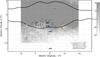 |
Fig. 1 Location of the five analyzed fields: B3, BW, B6, BL, and SW. All of these except SW are previously analyzed in, for example, Lecureur et al. (2007). These locations are compared to the COBE/DIRBE outline of the Galactic bulge (Weiland et al. 1994), the locations of the microlensed bulge dwarf stars of Bensby et al. (2013), and the high-resolution sample of the GIBS survey (González et al. 2015). Also shown is the extinction toward the bulge from the BEAM calculator1 based on González et al. (2011b, 2012) scaled to optical extinction (Cardelli et al. 1989). |
2. Observations
We observed 46 K giants in the Galactic bulge using the spectrometer FLAMES/UVES mounted on VLT. The basic data of our stars are listed in Table 1 and the Fig. 1 shows the location of our five fields (SW, B3, BW, B6, and BL) in comparison to the COBE/DIRBE outline of the Galactic bulge (Weiland et al. 1994), the locations of the microlensed bulge dwarfs of Bensby et al. (2013), and the high-resolution sample of the GIBS survey (González et al. 2015). As can be seen in Fig. 1, the new field in the Sagittarius Window (SW; (l,b) = (1.25,−2.65)) is closer to the Galactic center than the other previously analyzed fields. Just like the other observed fields, it is situated in a region where the optical extinction is lower than the surroundings. To go even closer to the Galactic center, infrared observations are needed because the optical extinction is high (see, e.g., Ryde & Schultheis 2015; Ryde et al. 2016); the corresponding infrared extinction in the bulge is essentially zero outside of the plane (for b< −1.5 or b> 1.5).
The spectra of the 35 stars in the B3, BW, B6, and BL fields analyzed here are the same as were analyzed for O in Zoccali et al. (2006), Na, Mg, and Al in Lecureur et al. (2007), Mn in Barbuy et al. (2013), and Ba, La, Ce, Nd, and Eu in Van der Swaelmen et al. (2016). These observations were carried out May–August 2003–2004. Since the fiber-array FLAMES was used in combination with UVES, seven stars could be observed in each pointing. Four spectra were excluded from the analysis because the determined stellar parameters are outside of the parameter space tested in Paper I: for one star, B3-b3, we derive a large log g of 3.23, making it possible to be a foreground disk star; for two stars, B3-b4 and B6-f2, we need to use atmospheric turbulence parameters outside of the ranges 1.0 <vmic< 2.0 and 1.0 <vmac< 8.0, which makes the determination of the surface gravity uncertain; and for one star, BW-f4, we derive a [Fe/H] =−1.55, which is lower than any of the stars analyzed in Paper I. We are not certain how well our stellar parameter determination works in this regime.
The 11 new stars in Sagittarius Window were observed in the same way using the same telescope, instrument, and setting in service mode during August 2011 (ESO program 085.B-0552(A)).
The total integration time in each setting was 5–12 h depending on extinction. The achieved signal-to-noise ratio (S/N) is listed in Table 2. The resolving power of the spectra is 47 000 and the spectra cover the region 5800 Å to 6800 Å.
Determined stellar parameters and abundances for the observed bulge giants.
3. Analysis and results
The spectra were analyzed using the exact same techniques and spectral lines used to analyze the solar neighborhood stars in Paper I. In short, the software Spectroscopy Made Easy (SME; Valenti & Piskunov 1996) was used to determine the stellar parameters and abundances via χ2 minimization of a synthetic and observed spectrum. In the analysis we used spherical symmetric, [α/Fe]-enhanced, LTE MARCS-models. Furthermore, NLTE corrections were used for the iron lines (Lind et al. 2012).
3.1. Reference sample
The main point of Paper I was to analyze a solar neighborhood reference sample of giant stars similar to the bulge stars analyzed here. The HR diagram of this solar neighborhood reference sample and the solar neighborhood dwarf stars of Bensby et al. (2014) are shown in the leftmost panel of Fig. 2.
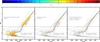 |
Fig. 2 HR diagrams for the program stars and the reference sample from Paper I. Also shown are the microlensed bulge dwarfs of Bensby et al. (2013) and their local disk comparison sample (Bensby et al. 2014) and the stellar parameters for bulge sample analyzed here as determined by Lecureur et al. (2007). As a guide for the eye, isochrones with [Fe/H] = 0.0 and ages 1−10 Gyr are plotted using solid light gray lines. Furthermore, one isochrone with [Fe/H] = −1.0 and age 10 Gyr, and one with [Fe/H] = +0.5 and age 10 Gyr are plotted using dotted dark gray lines (Bressan et al. 2012). |
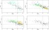 |
Fig. 3 [X/Fe] vs. [Fe/H] for the analyzed bulge giants and some previous works. The stars are color-coded as the corresponding fields in Fig. 1, and black diamonds representing the microlensed bulge dwarfs of Bensby et al. (2013), light green squares showing the abundances of Johnson et al. (2014), and golden stars showing the abundances of the high-resolution sample of the GIBS survey (González et al. 2015). We use A(O)⊙ = 8.69, A(Mg)⊙ = 7.60, A(Ca)⊙ = 6.34, A(Ti)⊙ = 4.95, and A(Fe)⊙ = 7.50 (Asplund et al. 2009). |
3.2. The bulge sample
In order to enable a strictly differential comparison to the reference sample, we redetermined the stellar parameters and abundances for the previously published B3-BW-B6-BL stars using the exact same purely spectroscopic analysis as for the solar neighborhood reference sample of Paper I. The resulting stellar parameters are plotted as a HR diagram in the middle panel of Fig. 2. For comparison, the parameters for the same stars as determined in Lecureur et al. (2007) are shown in the rightmost panel. As can be seen, the largest differences between the two sets of stellar parameters are seen in the surface gravities, where our results are spread out along the red giant branch; this is not shown in the previous stellar parameters of Lecureur et al. (2007), however. Furthermore, our results, in contrast to the older parameters, are sorted in [Fe/H] as expected in Fig. 2. This, together with the careful evaluation of the method used (in Paper I), gives us confidence in our determined stellar parameters.
The determined parameters and abundances are listed in Table 2. Furthermore, the determined abundances are shown in Fig. 3 together with the microlensed bulge dwarfs of Bensby et al. (2013), the abundances of Johnson et al. (2014), and the GIBS survey (González et al. 2015).
4. Discussion
Because we are not able to see any trends in metallicity nor abundances across the different fields, in the following we handle the entire sample as a bulge sample. To see possible trends more stars in every field are needed.
It is hard to estimate the age of giant stars, but from the isochrones in Fig. 2, one can see a slight splitting up with respect of age for the giants with highest gravities (close to log g = 3). This might possibly be visible in a slight split/spread of the solar metallicity (orange in the plot) stars of the solar neighborhood sample, while the same effect is not clearly visible in the bulge sample, which is expected since the bulge stars are predominately old (e.g., Clarkson et al. 2008; but see also Bensby et al. 2013). From Fig. 2 it is also obvious that the bulge stars generally are more metal rich than the giants found in the solar neighborhood.
4.1. Comparison to other studies
From Fig. 3, one can see that our stars and the microlensed dwarfs (Bensby et al. 2013) have very similar trends. However, our trends possibly show marginally higher scatter. Our [O/Fe] versus [Fe/H] trend is much less scattered and less steep than that of Johnson et al. (2014). The differences are likely due to the large uncertainties inherent in determining the oxygen abundance from the 6300 Å [O i] line in the relatively low-resolution spectra of Johnson et al. (2014). For example, González et al. (2011a) entirely avoid determining the oxygen abundance from the exact same data because of these uncertainties. When it comes to our [Ca/Fe] versus [Fe/H] trend, it is much tighter and less alpha enhanced than the corresponding trends of Johnson et al. (2014) and González et al. (2015). These differences may be attributed to our stellar parameters, which likely are more accurate because of our larger wavelength coverage, higher resolution, and thorough tests of our method in Paper I. On the other hand, the [Mg/Fe] versus [Fe/H] trends of Johnson et al. (2014) and González et al. (2015) are less alpha enhanced and tighter than ours. It is not clear why our data show a larger scatter; all three works use the same three Mg i lines around 6318–19 Å and our data has higher resolution, which suggests that our data, at least theoretically, should be of higher quality. However, these three lines have several difficulties. First of all, these lines have uncertain gf values; Johnson et al. (2014) and González et al. (2015) use astrophysical values and we use the (very similar) results of Pehlivan Rhodin et al. (2017). Second, the lines are affected by an autoionizing Ca i line, producing a very wide depression of the spectrum. Johnson et al. (2014), like us, solve this problem by setting a local pseudo-continuum around the Mg i lines, while González et al. (2015) both model the autoionizing Ca i line using their determined Ca abundance, and place a local continuum to get rid of possible residual mismatches between the observed and synthetic spectra. Third, the lines are in a region that is affected by telluric lines. Johnson et al. (2014) remove these by division by an observed “telluric” spectrum, while both González et al. (2015) and this work simply avoid using the Mg lines that are visibly affected by telluric contamination. To conclude, a possible explanation for our more scattered [Mg/Fe] versus [Fe/H] trend might be that the (necessary) lower S/N of our higher resolution data makes the continuum placement more difficult; our tendency to derive higher [Mg/Fe] might be due to the lower S/N, making it harder to identify and avoid telluric lines; this implies that we would derive too high magnesium abundances in the cases in which we possibly fail to identify a telluric line.
Several previous studies, but certainly not all, have found different trends for [O/Fe] and [Mg/Fe] in the bulge. The possibly different trends might suggest that there have been a higher degree of massive stars in the bulge as compared to the solar neighborhood. One example of a work finding different oxygen and magnesium trends in the bulge is Lecureur et al. (2007), who used 35 of the same spectra as in our study. The fact that we analyze the exact same spectra enables an interesting comparison between the two analyses. Therefore, we plotted the oxygen abundances of Zoccali et al. (2006), which are the very same abundances presented in Lecureur et al. (2007), along with the magnesium abundances of Lecureur et al. (2007) in Fig. 4. Our reanalysis shows a similar, but slightly less scattered, oxygen trend as in Zoccali et al. (2006), while our magnesium trend is lower in [Mg/Fe] for [Fe/H] >−0.5, showing a rather thick disk-like trend that is at odds with what is found in Lecureur et al. (2007). We believe that most of these differences can be attributed not only to our new all-spectroscopic stellar parameters, but also to the different handling of the autoionizing Ca i line affecting the derived magnesium abundances. Lecureur et al. (2007) model this line to reduce its influence in spite of its uncertain spectroscopic data, while we avoid synthesizing it and instead place a local pseudo-continuum around the three Mg i lines; for examples of their modeling of this line, see Figs. 3 and 5 in Lecureur et al. (2007).
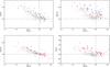 |
Fig. 4 [X/Fe] vs. [Fe/H]. From our investigation of the impact of S/N on the abundances (Paper I, Fig. 2), we conclude that the uncertainties of the abundances are multiplied for S/N< 20. Therefore, we plot our results for the bulge spectra with S/N> 20 using red dots and the results from those with S/N< 20 using pink squares. The solar neighborhood reference sample of giants from Paper I is plotted in gray. Previous abundances for the exact same spectra from Zoccali et al. (2006; oxygen) and Lecureur et al. (2007; magnesium) are plotted using blue diamonds. |
There are several ongoing large spectroscopic projects surveying the entire Galaxy and including the bulge. For example the APOGEE survey (Eisenstein et al. 2011) has observed a wealth of stars (over 150 000) with several fields toward the bulge. The APOGEE survey has the advantage of observing in the H band, reducing the problem of extinction of light due to dust. However, the rather small diameter of the telescope used means that the stars that actually are in the bulge are the most luminous giants, which are the hardest to analyze. As of yet there have been no APOGEE papers on the bulge, although one paper has addressed the very special stellar population of the absolute Galactic center (Schultheis et al. 2015).
The Gaia ESO-survey has some fields in the bulge, but has so far not published any comparison between the alpha elemental trends of the disk and bulge, but only an investigation on the metallicity and kinematic trends of the bulge (Rojas-Arriagada et al. 2014).
4.2. Comparison to the solar neighborhood sample
As has been mentioned several times before, the abundance trends found in the bulge must be compared to similarly determined trends in the disk. Most importantly to minimize systematic differences, the type of stars and spectral lines used in the analysis should be the same. Ideally the quality of the spectra should also be the same, but this is harder to obtain; it is impossible to obtain the same S/N for the faint bulge giants as for the bright nearby disk giants and, given the difference in magnitude, it is possible that the same telescope/spectrometer cannot be used in both cases. In our case we used FIES (Telting et al. 2014) at NOT and data retrieved from the NARVAL and ESPaDOnS spectral archive PolarBase (Petit et al. 2014) to collect spectra for the solar neighborhood sample of Paper I, while we used UVES/FLAMES at VLT for the bulge sample. The FIES and PolarBase spectra have a resolving power of 67 000 and 65 000, respectively, and high S/N (typically around 100), while the UVES/FLAMES spectra have R ~ 47 000 and much lower S/N (see Table 2). The effect of this difference in spectral quality is expected to manifest itself as more scatter in the bulge trends.
In Fig. 4, in which we compare the abundance trends from our solar neighborhood sample of Paper I to that of the bulge stars of this article, it is obvious that the abundance trends in the bulge are indeed not as tight as the trends from the solar neighborhood. Since the type of stars analyzed and the lines used are the same, this larger spread can only be attributed to lower S/N in the bulge-observations. Comparing Table 2 and to Fig. 2 in Paper I, in which we investigate the impact of S/N on the stellar parameters and abundances, all SW stars are expected to have an uncertainty in the [X/Fe] abundance ratio of around 0.2 dex (standard deviation) stemming from the S/N alone. The B3-BW-B6-BL stars generally have higher S/N and are expected to show lower uncertainties owing to the S/N, which is in general around 0.1 dex (standard deviation) for the [X/Fe] abundance ratios. As mentioned earlier, the scatter in the [Mg/Fe] trend for the bulge stars seems higher than for the other elements, and is possibly slightly enhanced compared to the thick disk, which is not seen for the other elements. This strongly suggests that the larger scatter in [Mg/Fe] for the bulge stars is linked to both the low S/N making it hard to place the continuum and identify telluric lines in the spectrum.
Comparing the abundance trends of Fig. 4, we find the bulge trends to follow generally the corresponding trends of the local thick disk. However, in the case of magnesium, calcium, and titanium, it is possible that the bulge trends trace the upper envelopes of the thick disk trends, while the bulge oxygen trend seems to follow the lower envelope of the corresponding local thick disk trend (or upper envelope of the local thin disk trend). These lower oxygen abundances could potentially be explained by the lower S/N of the bulge stars: from Fig. 2 in Paper I, an asymmetry for the lowest S/N is seen in the oxygen abundance, suggesting that lower oxygen abundances are derived for lower S/N. In general, the oxygen abundance is expected to be more sensitive to the lower quality of the spectra, since it is based on a single line in contrast to the magnesium, calcium, and titanium abundances. On the other hand, the oxygen and calcium abundance trends are the tightest of the four, suggesting that the determined surface gravity is precise; the oxygen and calcium abundances are mainly dependent on the surface gravity, as is shown in Table 3 in Paper I for oxygen, and is evident in the case of calcium since it is used to constrain the surface gravity.
In spite of the slight differences of oxygen and magnesium when comparing our bulge sample to our local disk sample in Fig. 4, we cannot see any evidence for [O/Fe] and [Mg/Fe] showing different trends in our bulge data; see Fig. 5. The [O/Mg] in our local disk sample is around zero for all metallicities, while the [O/Mg] in our bulge data is negative, but still constant. This difference might be on account of our oxygen abundances in the bulge possibly being systematically too low on account of the lower S/N in the bulge spectra. Furthermore, slightly higher magnesium abundances in the bulge trend can possibly be attributed to difficulties in avoiding telluric lines in the more noisy bulge spectra, as mentioned earlier.
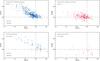 |
Fig. 5 Left panels: [O/Fe] and [Mg/Fe] vs. [Fe/H] for the solar neighborhood and bulge giants, respectively. Right panels: [O/Mg] vs. [Fe/H] for the solar neighborhood and bulge giants, respectively. |
From Fig. 4, we see no clear evidence for different positions of the knees of the bulge population and thick disk population, thereby corroborating González et al. (2015), but the conclusion is weak. To make a firmer statement, we would ideally need a larger bulge sample extending to lower metallicities and more thick disk stars in our local sample.
To resolve the question about the possible higher knee in the alpha elemental abundance plots for the bulge as compared to the local thick disk, one would need two decent sized stellar samples: one from the bulge and one from the local disk. This can be reached in several ways, some of which are listed below:
-
The investigation of Bensbyet al. (2013) has a large andrepresentative sample of 714 local dwarf stars,while the bulge sample is much smaller with58 microlensed dwarfs. Ideally, the bulge sampleshould be enlarged, but with the unpredictability of themicrolensing events, this is not readily carried out. Also, the typeof stars in the two samples are not exactly the same with the localsample being F and G dwarf stars, while the bulgesample contains several slightly cooler subgiant stars; seeFig. 2.
-
The investigations of Johnson et al. (2014) and González et al. (2015), on the other hand, both have large bulge samples of hundreds of giant stars with very tight and unscattered [Mg/Fe]-trends; see Fig. 3. However, they both have small similarly analyzed local disk samples of giants to which they contrast their bulge trends. Furthermore, their other α elements show larger scatter than our trends.
-
Our investigation has a local disk sample of 291 giants, but would benefit from having more thick-disk stars. The bulge sample consists of 46 giants of very similar types as the local sample; see Fig. 2.
The strategy used here, of observing K giants in the optical with high-resolution spectroscopy, has the upside that it is easy to find and observe suitable, very similar local disk stars and also telescopes/instruments with which to carry out these observations. The downside is the long integration times needed for the bulge observations. However, FLAMES/UVES offers the ability to observe seven stars simultaneously, resulting in about one hour telescope time per star, similar to the amount of time spent per microlensed dwarf star in Bensby et al. (2013).
For the future, a similar methodology as presented here but performed in the near-IR H and/or K bands would be rewarding. This is indeed possible now with the new cross-dispersed high-resolution, near-IR spectrometers recently available or in planning stages (see, e.g., Park et al. 2014; Origlia et al. 2014), but to accomplish this a serious effort in exploring usable and reliable spectral features in the near-IR needs to be addressed.
5. Conclusions
We determined the abundances of oxygen, magnesium, calcium, and titanium in a sample of 46 bulge K giants, 35 of which were analyzed for oxygen and magnesium in previous works (Zoccali et al. 2006; Lecureur et al. 2007), and compare the abundances to those of 291 similarly analyzed K giants in the solar neighborhood.
To conclude, our reanalysis of the bulge oxygen abundances from Zoccali et al. (2006) and the magnesium abundances from Lecureur et al. (2007) result in similar oxygen trends, while we do not see the high [Mg/Fe] values for the highest [Fe/H] stars. Thereby we contradict Lecureur et al. (2007) and their claim that the oxygen and magnesium trends are very different in the bulge. Furthermore, the question of a possible shift in position of the knee in the [α/Fe] plot in the bulge as compared to the local disk is not unambiguously answered.
Acknowledgments
This research has been partly supported by the Royal Physiographic Society in Lund, Stiftelsen Walter Gyllenbergs fond. N.R. acknowledges support from the Swedish Research Council, VR (project number 2014–5640). M.Z. acknowledges support by the Ministry of Economy, Development, and Tourism’s Millennium Science Initiative through grant IC120009, awarded to The Millennium Institute of Astrophysics (MAS), by Fondecyt Regular 1150345 and by the BASAL-CATA Center for Astrophysics and Associated Technologies PFB-06. This publication made use of the SIMBAD database, operated at CDS, Strasbourg, France, NASA’s Astrophysics Data System, and the VALD database, operated at Uppsala University, the Institute of Astronomy RAS in Moscow, and the University of Vienna.
References
- Alves-Brito, A., Meléndez, J., Asplund, M., Ramírez, I., & Yong, D. 2010, A&A, 513, A35 [NASA ADS] [CrossRef] [EDP Sciences] [Google Scholar]
- Asplund, M., Grevesse, N., Sauval, A. J., & Scott, P. 2009, ARA&A, 47, 481 [NASA ADS] [CrossRef] [Google Scholar]
- Barbuy, B., Hill, V., Zoccali, M., et al. 2013, A&A, 559, A5 [NASA ADS] [CrossRef] [EDP Sciences] [Google Scholar]
- Bensby, T., Feltzing, S., & Lundström, I. 2003, A&A, 410, 527 [NASA ADS] [CrossRef] [EDP Sciences] [Google Scholar]
- Bensby, T., Feltzing, S., Lundström, I., & Ilyin, I. 2005, A&A, 433, 185 [NASA ADS] [CrossRef] [EDP Sciences] [Google Scholar]
- Bensby, T., Yee, J. C., Feltzing, S., et al. 2013, A&A, 549, A147 [NASA ADS] [CrossRef] [EDP Sciences] [Google Scholar]
- Bensby, T., Feltzing, S., & Oey, M. S. 2014, A&A, 562, A71 [NASA ADS] [CrossRef] [EDP Sciences] [Google Scholar]
- Bressan, A., Marigo, P., Girardi, L., et al. 2012, MNRAS, 427, 127 [NASA ADS] [CrossRef] [Google Scholar]
- Cardelli, J. A., Clayton, G. C., & Mathis, J. S. 1989, ApJ, 345, 245 [NASA ADS] [CrossRef] [Google Scholar]
- Clarkson, W., Sahu, K., Anderson, J., et al. 2008, ApJ, 684, 1110 [NASA ADS] [CrossRef] [Google Scholar]
- Dékány, I., Minniti, D., Catelan, M., et al. 2013, ApJ, 776, L19 [NASA ADS] [CrossRef] [Google Scholar]
- Eisenstein, D. J., Weinberg, D. H., Agol, E., et al. 2011, AJ, 142, 72 [Google Scholar]
- González, O. A., Rejkuba, M., Zoccali, M., et al. 2011a, A&A, 530, A54 [NASA ADS] [CrossRef] [EDP Sciences] [Google Scholar]
- González, O. A., Rejkuba, M., Zoccali, M., Valenti, E., & Minniti, D. 2011b, A&A, 534, A3 [NASA ADS] [CrossRef] [EDP Sciences] [Google Scholar]
- González, O. A., Rejkuba, M., Zoccali, M., et al. 2012, A&A, 543, A13 [NASA ADS] [CrossRef] [EDP Sciences] [Google Scholar]
- González, O. A., Zoccali, M., Vásquez, S., et al. 2015, A&A, 584, A46 [NASA ADS] [CrossRef] [EDP Sciences] [Google Scholar]
- Huber, D., Silva Aguirre, V., Matthews, J. M., et al. 2014, ApJS, 211, 2 [NASA ADS] [CrossRef] [Google Scholar]
- Johnson, C. I., Rich, R. M., Kobayashi, C., Kunder, A., & Koch, A. 2014, AJ, 148, 67 [NASA ADS] [CrossRef] [Google Scholar]
- Jönsson, H., Ryde, N., Nordlander, T., et al. 2017, A&A, 598, A100 (Paper I) [NASA ADS] [CrossRef] [EDP Sciences] [Google Scholar]
- Kunder, A., Koch, A., Rich, R. M., et al. 2012, AJ, 143, 57 [NASA ADS] [CrossRef] [Google Scholar]
- Kunder, A., Rich, R. M., Koch, A., et al. 2016, ApJ, 821, L25 [NASA ADS] [CrossRef] [Google Scholar]
- Lecureur, A., Hill, V., Zoccali, M., et al. 2007, A&A, 465, 799 [NASA ADS] [CrossRef] [EDP Sciences] [Google Scholar]
- Lind, K., Bergemann, M., & Asplund, M. 2012, MNRAS, 427, 50 [NASA ADS] [CrossRef] [Google Scholar]
- McWilliam, A., & Zoccali, M. 2010, ApJ, 724, 1491 [NASA ADS] [CrossRef] [Google Scholar]
- Mozurkewich, D., Armstrong, J. T., Hindsley, R. B., et al. 2003, AJ, 126, 2502 [NASA ADS] [CrossRef] [Google Scholar]
- Nataf, D. M., Udalski, A., Gould, A., Fouqué, P., & Stanek, K. Z. 2010, ApJ, 721, L28 [NASA ADS] [CrossRef] [Google Scholar]
- Ness, M., Freeman, K., Athanassoula, E., et al. 2012, ApJ, 756, 22 [NASA ADS] [CrossRef] [Google Scholar]
- Ness, M., Freeman, K., Athanassoula, E., et al. 2013, MNRAS, 432, 2092 [NASA ADS] [CrossRef] [Google Scholar]
- Origlia, L., Oliva, E., Baffa, C., et al. 2014, in Proc. SPIE, INAF – Osservatorio Astronomico di Bologna (Italy) (International Society for Optics and Photonics), 91471E–91471E–9 [Google Scholar]
- Park, C., Jaffe, D. T., Yuk, I.-S., et al. 2014, in Proc. SPIE, 9147, 9147D [Google Scholar]
- Pehlivan Rhodin, A., Hartman, H., Nilsson, H., & Jönsson, P. 2017, A&A, 598, A102 [NASA ADS] [CrossRef] [EDP Sciences] [Google Scholar]
- Petit, P., Louge, T., Théado, S., et al. 2014, PASP, 126, 469 [NASA ADS] [CrossRef] [Google Scholar]
- Reddy, B. E., Lambert, D. L., & Allen de Prieto, C. 2006, MNRAS, 367, 1329 [NASA ADS] [CrossRef] [Google Scholar]
- Rich, R. M., Reitzel, D. B., Howard, C. D., & Zhao, H. 2007, ApJ, 658, L29 [NASA ADS] [CrossRef] [Google Scholar]
- Rich, R. M., Origlia, L., & Valenti, E. 2012, ApJ, 746, 59 [NASA ADS] [CrossRef] [Google Scholar]
- Rojas-Arriagada, A., Recio-Blanco, A., Hill, V., et al. 2014, A&A, 569, A103 [NASA ADS] [CrossRef] [EDP Sciences] [Google Scholar]
- Ryde, N., & Schultheis, M. 2015, A&A, 573, A14 [NASA ADS] [CrossRef] [EDP Sciences] [Google Scholar]
- Ryde, N., Gustafsson, B., Edvardsson, B., et al. 2010, A&A, 509, A20 [NASA ADS] [CrossRef] [EDP Sciences] [Google Scholar]
- Ryde, N., Schultheis, M., Grieco, V., et al. 2016, AJ, 151, 1 [NASA ADS] [CrossRef] [Google Scholar]
- Saha, K., Martinez-Valpuesta, I., & Gerhard, O. 2012, MNRAS, 421, 333 [NASA ADS] [Google Scholar]
- Schultheis, M., Cunha, K., Zasowski, G., et al. 2015, A&A, 584, A45 [NASA ADS] [CrossRef] [EDP Sciences] [Google Scholar]
- Telting, J. H., Avila, G., Buchhave, L., et al. 2014, Astron. Nachr., 335, 41 [NASA ADS] [CrossRef] [Google Scholar]
- Thygesen, A. O., Frandsen, S., Bruntt, H., et al. 2012, A&A, 543, A160 [NASA ADS] [CrossRef] [EDP Sciences] [Google Scholar]
- Valenti, J. A., & Piskunov, N. 1996, A&AS, 118, 595 [NASA ADS] [CrossRef] [EDP Sciences] [Google Scholar]
- Van der Swaelmen, M., Barbuy, B., Hill, V., et al. 2016, A&A, 586, A1 [NASA ADS] [CrossRef] [EDP Sciences] [Google Scholar]
- Weiland, J. L., Arendt, R. G., Berriman, G. B., et al. 1994, ApJ, 425, L81 [NASA ADS] [CrossRef] [Google Scholar]
- Zoccali, M., Lecureur, A., Barbuy, B., et al. 2006, A&A, 457, L1 [NASA ADS] [CrossRef] [EDP Sciences] [Google Scholar]
- Zoccali, M., González, O. A., Vásquez, S., et al. 2014, A&A, 562, A66 [NASA ADS] [CrossRef] [EDP Sciences] [Google Scholar]
All Tables
All Figures
|
Fig. 1 Location of the five analyzed fields: B3, BW, B6, BL, and SW. All of these except SW are previously analyzed in, for example, Lecureur et al. (2007). These locations are compared to the COBE/DIRBE outline of the Galactic bulge (Weiland et al. 1994), the locations of the microlensed bulge dwarf stars of Bensby et al. (2013), and the high-resolution sample of the GIBS survey (González et al. 2015). Also shown is the extinction toward the bulge from the BEAM calculator1 based on González et al. (2011b, 2012) scaled to optical extinction (Cardelli et al. 1989). |
| In the text | |
|
Fig. 2 HR diagrams for the program stars and the reference sample from Paper I. Also shown are the microlensed bulge dwarfs of Bensby et al. (2013) and their local disk comparison sample (Bensby et al. 2014) and the stellar parameters for bulge sample analyzed here as determined by Lecureur et al. (2007). As a guide for the eye, isochrones with [Fe/H] = 0.0 and ages 1−10 Gyr are plotted using solid light gray lines. Furthermore, one isochrone with [Fe/H] = −1.0 and age 10 Gyr, and one with [Fe/H] = +0.5 and age 10 Gyr are plotted using dotted dark gray lines (Bressan et al. 2012). |
| In the text | |
|
Fig. 3 [X/Fe] vs. [Fe/H] for the analyzed bulge giants and some previous works. The stars are color-coded as the corresponding fields in Fig. 1, and black diamonds representing the microlensed bulge dwarfs of Bensby et al. (2013), light green squares showing the abundances of Johnson et al. (2014), and golden stars showing the abundances of the high-resolution sample of the GIBS survey (González et al. 2015). We use A(O)⊙ = 8.69, A(Mg)⊙ = 7.60, A(Ca)⊙ = 6.34, A(Ti)⊙ = 4.95, and A(Fe)⊙ = 7.50 (Asplund et al. 2009). |
| In the text | |
|
Fig. 4 [X/Fe] vs. [Fe/H]. From our investigation of the impact of S/N on the abundances (Paper I, Fig. 2), we conclude that the uncertainties of the abundances are multiplied for S/N< 20. Therefore, we plot our results for the bulge spectra with S/N> 20 using red dots and the results from those with S/N< 20 using pink squares. The solar neighborhood reference sample of giants from Paper I is plotted in gray. Previous abundances for the exact same spectra from Zoccali et al. (2006; oxygen) and Lecureur et al. (2007; magnesium) are plotted using blue diamonds. |
| In the text | |
|
Fig. 5 Left panels: [O/Fe] and [Mg/Fe] vs. [Fe/H] for the solar neighborhood and bulge giants, respectively. Right panels: [O/Mg] vs. [Fe/H] for the solar neighborhood and bulge giants, respectively. |
| In the text | |
Current usage metrics show cumulative count of Article Views (full-text article views including HTML views, PDF and ePub downloads, according to the available data) and Abstracts Views on Vision4Press platform.
Data correspond to usage on the plateform after 2015. The current usage metrics is available 48-96 hours after online publication and is updated daily on week days.
Initial download of the metrics may take a while.