| Issue |
A&A
Volume 598, February 2017
|
|
|---|---|---|
| Article Number | A31 | |
| Number of page(s) | 18 | |
| Section | Interstellar and circumstellar matter | |
| DOI | https://doi.org/10.1051/0004-6361/201628987 | |
| Published online | 27 January 2017 | |
The nearby interstellar medium toward α Leo
UV observations and modeling of a warm cloud within hot gas
1 Aix-Marseille Univ., CNRS, LAM (Laboratoire d’Astrophysique de Marseille), 13388 Marseille Cedex 13, France
e-mail: This email address is being protected from spambots. You need JavaScript enabled to view it.
2 Department of Astrophysical Sciences, Princeton University Observatory, Princeton, NJ 08544, USA
e-mail: This email address is being protected from spambots. You need JavaScript enabled to view it.
Received: 23 May 2016
Accepted: 7 September 2016
Abstract
Aims. Our aim is to characterize the conditions in the nearest interstellar cloud.
Methods. We analyze interstellar absorption features in the full UV spectrum of the nearby (d = 24 pc) B8 IVn star α Leo (Regulus). Observations were obtained with STIS at high resolution and high signal-to-noise ratio by the HST ASTRAL Treasury program. We derive column densities for many key atomic species and interpret their partial ionizations.
Results. The gas in front of α Leo exhibits two absorption components. The main one is kinematically identified as the local interstellar cloud (LIC) that surrounds the Sun. The second component is shifted by +5.6 km s-1 relative to the main component, in agreement with results for other lines of sight in this region of the sky, and shares its ionization and physical conditions. The excitation of the C II fine-structure levels and the ratio of Mg I to Mg II reveal a temperature T = 6500 (+750, −600) K and electron density n(e) = 0.11 (+0.025, −0.03) cm-3. Our investigation of the ionization balance yields the ion fractions for 10 different atoms and indicates that about 1/3 of the hydrogen atoms are ionized. Metals are significantly depleted onto grains, with sulfur showing [S/H] ~ −0.27. N(H I) = 1.9 (+0.9, −0.6) × 1018 cm-3, which indicates that this partly neutral gas occupies only 2 to 8 parsecs (about 13%) of the space toward the star, with the remaining volume being filled with a hot gas that emits soft X-rays. We do not detect any absorption features from the highly ionized species that could be produced in an interface between the warm medium and the surrounding hot gas, possibly because of non-equilibrium conditions or a particular magnetic field orientation that reduces thermal conduction. Finally, the radial velocity of the LIC agrees with that of the Local Leo Cold Cloud, indicating that they may be physically related.
Key words: ISM: clouds / ISM: abundances / local insterstellar matter / ultraviolet: ISM / stars: individual: α Leo
© ESO, 2017
1. Introduction
Beginning with findings from the Copernicus satellite (Spitzer & Jenkins 1975), studies of ultraviolet absorption features appearing in the spectra of hot, rapidly rotating stars have yielded fundamental insights into the compositions and physical characters of different phases of the interstellar medium (Savage & Sembach 1996), along with the processes that influence them. With the exception of white dwarf stars and stars with spectral types A and cooler, nearly all of the targets are so distant that their sight lines traverse regions with characteristics that are substantially different from one another. As a consequence, the interstellar absorption features usually reveal a heterogeneous mix of the imprints of many different regions, which can only be separated by chance offsets in radial velocities.
Nearby stars offer an opportunity to explore a less cluttered situation, but they have the drawback that they represent only one or a few regions with very similar properties. Even so, recent investigations of our nearby environment have been very useful in revealing its dynamics (Redfield & Linsky 2008; Gry & Jenkins 2014, gas-phase composition (Lehner et al. 2003; Redfield & Linsky 2004a), ionization state (Jenkins et al. 2000), temperature, and turbulent velocities (Redfield & Linsky 2004b). In addition, Oegerle et al. (2005), Savage & Lehner (2006), and Barstow et al. (2010) have found evidence for the presence of a very hot medium in some nearby locations. A review of many findings on the local medium has been presented by Frisch et al. (2011).
The earlier UV studies of the local environment had to contend with some difficulties. White dwarf stars were once thought to have featureless spectra that could cleanly show interstellar lines, but subsequent investigations have revealed unexpectedly high metal abundances in the atmospheres of these narrow-line stars, caused by radiative levitation (Barstow et al. 2003) and pollution by the infall of circumstellar matter (Rafikov & Garmilla 2012; Barstow et al. 2014). These atmospheric metal-line features, along with ones arising from circumstellar matter, can create serious confusion when attempting to discern interstellar features (Lallement et al. 2011), but in a small percentage of cases the interstellar absorptions can be separated from the photospheric or circumstellar contributions (Barstow et al. 2010). For cool stars, a different problem emerges. Here, interstellar absorption features must be viewed on top of chromospheric emission features, a problem which forces one to have a good understanding of the shapes of the underlying emission profiles.
O and B type stars whose stellar features are broadened by rotation represent ideal targets for interstellar absorption line studies. This paper focuses on the UV spectrum of one such star, α Leo (Regulus), a bright (V = 1.40) B8 IVn star that was recently observed in a 230-orbit HST Cycle 21 Treasury Program (program ID = 13346, T. R. Ayres, PI) called the Advanced Spectral Library II: Hot Stars (ASTRAL). This observing program produced atlases of high-resolution, complete UV spectra of 21 diverse early-type stars. Our target α Leo, at a distance of 24 pc, is the nearest B-type main sequence or giant star in the sky. Its strong brightness in the ultraviolet and its high projected rotational velocity (vsini = 353 km s-1) make it an ideal target for investigating the local medium.
As we discuss in later sections of this paper, the spectrum of this star reveals important details on the density and degree of ionization of hydrogen atoms, the gas-phase abundances of certain elements, the temperature of the gas, along with the filling factor along the sight line for constituents that we can detect. Finally, at the Galactic coordinates ℓ = 226.4°, b = + 48.9°, α Leo samples a portion of the sky that has not been well sampled at close distances (Gry & Jenkins 2014; Malamut et al. 2014).
2. Our local environment
In broadest terms, the Sun is located in a specially rarefied region of the Galaxy. It is situated in a small, diffuse (nH I = 0.05−0.3 cm-3), warm medium, which itself is embedded in an irregularly shaped cavity of about 100 pc radius (Welsh et al. 2010; Lallement et al. 2014). This cavity is called the Local Bubble. It is almost devoid of neutral gas and is probably filled mostly with a hot (T ~ 106 to 107 K) tenuous, collisionally ionized gas that emits soft X-rays (Williamson et al. 1974; McCammon & Sanders 1990; Snowden et al. 1997, 2014).
It is generally recognized that the local interstellar cloud (LIC) that surrounds our heliospheric environment is partly ionized to a level ne/nH ~ 0.5 by the ambient EUV and X-ray radiation field that arises from stars (Vallerga 1998) and the surrounding hot gas (Slavin & Frisch 2008). In accord with previous findings by Redfield & Linsky (2004b), we show that the temperature of the gas is close to T ~ 7000 K, which is one of the stable phases that arises from the bifurcation due to the Field (1965) thermal instability (Wolfire et al. 2003). The magnetic field at distances greater than 1000 AU from the Sun has a strength of about 3 μG and is directed toward ℓ = 26.1°, b = 49.5°, according to an interpretation of results from the Interstellar Boundary Explorer (IBEX) by Zirnstein et al. (2016). The magnetic direction thus makes an angle of about 79° with respect to the direction toward α Leo.
The distance to the boundary between the LIC and the surrounding hot medium is not well determined, but it is probably of order 10 pc (Frisch et al. 2011; Gry & Jenkins 2014). It is therefore very likely that the sight line to α Leo penetrates this boundary. In principle, UV spectroscopic data should help us to understand the nature of this boundary: is it a conduction front where evaporation or condensation of warm gas is occurring (Cowie & McKee 1977; McKee & Cowie 1977; Ballet et al. 1986; Slavin 1989; Borkowski et al. 1990; Dalton & Balbus 1993)? Alternatively, could it be a turbulent mixing layer (TML), where, as the name implies, the existence of any shear in velocity between the phases creates instabilities and mechanically induced chaotic interactions (Begelman & Fabian 1990; Slavin et al. 1993; Kwak & Shelton 2010)? Observers have attempted to identify these processes chiefly by analyzing interstellar absorption features of ions that are most abundant at intermediate temperatures, such as Si IV, C IV, N V, and O VI, and then comparing their column density ratios with the theoretical predictions (Spitzer 1996; Sembach et al. 1997; Zsargó et al. 2003; Indebetouw & Shull 2004a,b; Lehner et al. 2011; Wakker et al. 2012). Such studies have been conducted over very long sight lines, where multiple interfaces may be found. Also, the signatures from interfaces possibly could be mixed with contributions from radiatively cooling gases. Papers that report these results give us information on the relative importance of different cases, but they tell us nothing about what happens within any single interface.
Inside the Local Bubble, there are a few isolated, dense clouds (Magnani et al. 1985; Begum et al. 2010). One such cloud attracted the attention of Verschuur (1969) and was studied further by Verschuur & Knapp (1971) because it had an unusually low 21-cm spin temperature and a low velocity dispersion. This cloud covering 22 deg2 in the Leo constellation and later estimated to be at a distance between 11 and 40 pc away from us was investigated using optical absorption features by Meyer et al. (2006) and in further detail by Peek et al. (2011), who named the cloud the Local Leo Cold Cloud (LLCC). The upper limit to its distance of 40 pc was established by (Meyer et al. 2006), who detected narrow Na I features toward two stars beyond the LLCC located at distances slightly over 40 pc. From HST STIS spectroscopy of stars behind this cloud, Meyer et al. (2012) analyzed the excitation of the fine-structure levels of C I and came to the remarkable conclusion that this cloud had an internal thermal pressure p/k ≈ 60 000 cm-3 K, which is considerably higher than estimates of p/k ≤ 10 000 cm-3K for the low density material inside the Local Bubble (Jenkins 2002, 2009; Frisch et al. 2011; Snowden et al. 2014). From its extraordinarily high thermal pressure and low 21-cm spin temperatures (13 to 22 K, Heiles & Troland 2003), this cloud presents an anomaly in the very diffuse context of the Local Bubble. Another interesting feature of this cloud is that it appears to coincide with a long string of other dense clouds that stretches across 80° in the sky (Haud 2010).
Our target α Leo is separated in projection by only about 4° from the LLCC. In fact, Peek et al. (2011) claimed that the very weak Ca II absorption feature in the spectrum of α Leo arises from the outermost portions of the LLCC, and therefore proposed that the LLCC distance upper limit be determined by the distance to the star α Leo. However we argue later that this component is likely to be produced by the LIC surrounding the Sun.
3. Observations and spectral analysis
3.1. HST-STIS data
Our spectrum was recorded with the E140H and E230H echelle modes at a spectral resolution λ/ Δλ ≈ 114 000 over the wavelength interval 1164 to 3045 Å. Many of the observations in the ASTRAL program were performed with the neutral density (ND) 0.2 × 0.05 arcsec entrance slit because the stars were very bright. This had to be done for α Leo. This slit is narrower than the standard 0.2 × 0.09 arcsec slit. Initially, we used the CALSTIS reduction package to process the data in a mode that recognized intensities within half pixels of the MAMA detector in order to retrieve the full wavelength resolution of the original data. However, we found that the very modest gain in resolution over the standard full pixel sampling was more than offset by the compromises from the greater uncertainties in the wavelength calibration and the zero-flux level determinations. We therefore decided to use simply the normal spectral sampling provided by the Mikulski Archive for Space Telescopes (MAST), which had better calibration files and improved control over the systematic errors.
With a few exceptions, we did not perform multi-exposure co-additions. For multiple exposures or wavelengths where there were order overlaps, we retained each individual spectrum segment for analysis so that we could avoid the misleading effects that arise from the interpolated resamplings, which introduce correlated noise in the spectra. Our independent treatments of duplicate spectral coverages secured separate error estimates and enabled us to obtain reliable estimates of the χ2 values which we could then combine in the ultimate minimization process for the line fitting. This also maintains the full resolution, since there is no resolution degradation introduced by interpolation of the wavelength grids or slight wavelength shifts over the different exposures. We found that for the strongest saturated lines we could sense slight errors in the derivations for the zero-flux levels. Thus, by keeping the different exposures separate we could correct for these errors individually and avoid systematic errors that might be hidden in the co-added spectra. The only cases where we had to use co-addition was for the Lyman-α profile discussed in Sect. 6.5, where the noise is so high that exposures cannot be reliably interpreted individually, as well as to derive column density upper limits for the undetected lines C iv, N v, Al iii, Si iii, Si iv and S iii.
3.2. Copernicus data
Our target star α Leo was one of the first set of stars observed in 1973 with the Copernicus satellite (Rogerson et al. 1973a). The results from these initial observations were reported by Rogerson et al. (1973b) in their study of what they called the “intercloud” medium. While working on the STIS data, we realized that more extensive Copernicus spectra were acquired in 1977, which have not yet been published. They included the O i line at 1039 Å, which is weaker and hence less saturated than the line at 1302 Å that we obtained with STIS. This weaker line was therefore quite beneficial in constraining the column density of O i. In addition, the Copernicus spectra covered the N ii 1084 Å line and the two Ar i lines at 1048 and 1066 Å, all of which are outside the wavelength coverage of STIS. At the time of the observations taken in 1977, the stray light was blocked and the only sources of background were charged particles and scattered light from the grating, making the background easier to correct than with the earlier published data.
We downloaded the co-added spectra from the MAST archive and used them to supplement our STIS data. We estimated background corrections for the Copernicus spectra through the use of Eq. (2) of Bohlin (1975), which expresses the scattered light level in the U1 tube at a wavelength λ in counts according to the relation ![Mathematical equation: \begin{equation} {\rm G}_1(\lambda) = 0.02 [{\rm U}_1(1200 \pm 200)] + 0.067 [{\rm U}_1(\lambda) \pm 12], \end{equation}](/articles/aa/full_html/2017/02/aa28987-16/aa28987-16-eq31.png) (1)where the brackets indicate an average perceived count level over the wavelength range specified. According to Bohlin (1975) the worst-case error is 2% of the continuum. For the absorption feature of N II depicted in Fig. 1 the background is thus 56.8 ± 7.2. It is 24.6 ± 4 for O i 1039 Å, 39.7 ± 8.8 for O i 1302 Å, 49.10 ± 18 for Ar i 1066 Å and 36.4 ± 9 for Ar i 1048 Å. The uncertainties in the background levels are the principal sources of error for the column densities that we derived. (The panels of Fig. 1 show the corrected count rates.)
(1)where the brackets indicate an average perceived count level over the wavelength range specified. According to Bohlin (1975) the worst-case error is 2% of the continuum. For the absorption feature of N II depicted in Fig. 1 the background is thus 56.8 ± 7.2. It is 24.6 ± 4 for O i 1039 Å, 39.7 ± 8.8 for O i 1302 Å, 49.10 ± 18 for Ar i 1066 Å and 36.4 ± 9 for Ar i 1048 Å. The uncertainties in the background levels are the principal sources of error for the column densities that we derived. (The panels of Fig. 1 show the corrected count rates.)
3.3. Spectral analysis: multi-element, multi-component profile fitting
To derive the characteristics of the interstellar components, i.e. column density N, velocity v, temperature T and turbulence bturb, we compared the observed line profiles with theoretical ones that represent the convolution of a Voigt profile with the instrumental line spread function (LSF). This comparison was performed with the use of the profile fitting software “Owens.f” developed in the 1990’s by Martin Lemoine and the French FUSE team. For all species, we adopted the f-values listed by Morton (2003).
The software enables one to simultaneously fit several lines of the same element, as well as lines from different elements. It also provides for the existence of several velocity components that can be fitted simultaneously yielding the characteristics of individual velocity components even when their profiles are blended together. The software therefore derives a global and consistent solution for all species with a common absorption velocity and common physical conditions, implying consistent broadening parameters. The fitting software breaks the line-broadening parameter (b-value, i.e.  projected along the sight line) into thermal broadening, which depends on the element mass, and non-thermal broadening (turbulence), which is the same for all elements in any given component. Therefore, fitting lines from elements of different masses simultaneously in principle enables the simultaneous measurement of temperature, turbulent velocity, mean velocity, and element column densities. All detected spectral lines used in this analysis are presented in Fig. 1 together with their fits.
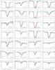 |
Fig. 1 Absorption line spectra in the line of sight to α Leo. Black histogram-style curves represent the observations, red solid lines are the best fits, green lines show the contributions from the two individual components that we could identify, and blue lines represent our reconstructions of the profiles before convolution with the instrumental LSF, i.e. the intrinsic interstellar profile. Stellar continua are shown in cyan. All fits have been performed simultaneously with the model for the line of sight with 2 components having same velocity, same temperature, and same turbulent broadening for all species. Copernicus spectra are labeled “Copernicus”, their flux scale is expressed in counts per 14 s; the remaining spectra are from HST/STIS and are indicated in the units 10-9 erg cm-2 s-1 Å-1. |
The spectra have not been normalized to the stellar continuum; instead the stellar profile is included in the fit as n + 1 free parameters for an n-degree polynomial (usually a straight line).
The LSFs applying to the Echelle gratings E140H and E230H are tabulated in the STIS Instrument Handbook for the two standard high-resolution slits 0.2 × 0.09 arcsec and 0.1 × 0.03 arcsec. They are represented by a sum of broad and narrow components whose FWHMs we derive in each case by performing a double-Gaussian fit to the tabulated LSFs. Since α Leo has been observed with the non-conventional slit 0.05ND for which the LSF has not been tabulated, and since its width is intermediate between the two standard slits, we make the assumption (recommended by STScI specialists) that the FWHMs for this slit can be interpolated from those resulting from the double-Gaussian fit to the two tabulated LSFs. As a result, we adopted for the low amplitude broad component a FWHM of 6 pixels and 5.11 pixels respectively for E140H and E230H data, and for the taller narrow component an FWHM that varies slightly with wavelength: 0.91 pixels at 1200 Å, 0.89 pixels at 1500 Å (E140H), and 1.50 pixels at 2400 Å (E230H). In essence, the spectra are undersampled according to the Nyquist criterion and thus are subject to aliasing. Our experiences with the half-pixel sampling indicated that this is not a serious problem. For Copernicus data, we have adopted a Gaussian LSF with a FWHM of 0.062 at 1302 Å and 0.051 for the other lines, corresponding to a resolution of 20 000 everywhere.
According to the STIS Instrument Handbook, the wavelength accuracy across exposures is 0.2–0.5 pixels. We do observe slight velocity variations in the spectra. Therefore, when we fit the spectra we allow for a free velocity shift between the different wavelength windows that cover different spectral lines or for identical spectral lines in different orders or exposures. The resulting velocity shifts have a dispersion close to 0.5 km s-1, so they are indeed generally lower than 0.5 pixel or 0.66 km s-1, except in rare cases such as near 1304 Å in order 12 of both E140H-1271 Å exposures, where the measured wavelength shift is ~+0.9 km s-1 at the position of the O i* and Si ii lines.
We can check on the heliocentric velocities of the interstellar components by measuring the observed velocities of the telluric absorption features of O i that originate from oxygen atoms in the Earth’s upper atmosphere. Such features should be offset from the heliocentric velocities by a correction listed in the V_HELIO keyword given in the data headers. On our reference O i spectrum (not allowed to shift in wavelength during the fit process) for which the keyword V_HELIO = 22.23 km s-1, we measure a telluric velocity of −21.21 km s-1. From this offset we derive an absolute offset ΔV = 1.02km s-1 that we subsequently subtract from the fit results to ascertain the absolute velocities of the interstellar components1.
The Copernicus data have a much larger velocity uncertainty caused by changes in the spectrometer temperatures (whose values are not available in the archive). The fits to the Copernicus lines therefore also allow a free velocity shift that can be as high as 8 km s-1. For this reason, along with the lack of resolution, we had to declare that the allotments of column densities between the two principal velocity components are uncertain for lines that are only observed with Copernicus.
Results of the profile fitting for the two components in the α Leo sight line.
3.4. Results from profile fitting
The quality of the fits, and the error bars on column densities, have been computed using the Δχ2 method described e.g. in Hébrard et al. (2002). We performed several fits by fixing the column density of a given element X to a different value in each fit. In all of these fits, all other parameters are set free and we compute the best χ2 for each value of column density. Then plots of Δχ2 versus N(X) yield the 1, 2, or 3σ ranges for N(X).
The fits to highly saturated features, like C ii and to a lesser extent O i, are constrained by the fact that they are performed together with the less saturated lines and the requirement that all share a consistent solution. Because we make the assumption that all species share the same turbulence and temperature, we expect that the values of these quantities for the strong lines are relatively well constrained by unsaturated lines. We use this principle to determine the column densities of species exhibiting only strong lines, ones that would otherwise be impossible to measure with any reasonable accuracy.
The column densities arising from the fits are listed in Table 1. The quoted uncertainty intervals include the effects of wavelength calibration uncertainties, as well as errors in the stellar continuum or detector zero-level placements, since variations of these three factors are permitted in the fit. The uncertainties however do not take into account uncertainty on our knowledge of the LSF, but we have checked that at the level of accuracy to which the LSF is known, the effects of such uncertainties are negligible.
We have used co-added spectra to derive upper limits for the column densities of undetected species in the following lines: C iv 1548 and 1550 Å, N v 1238 and 1242 Å, Al iii 1854 and 1862 Å, Si iii 1206 Å, Si iv 1393 and 1402 Å and S iii 1190 Å. At a most fundamental level, uncertainties caused by photon counting noise can alter the shape of an absorption feature, and a means for estimating an error from this process for an equivalent width has been outlined by Jenkins et al. (1973). Adding to this uncertainty is the error in establishing a continuum level. For the special cases associated with weak, broad features that might be expected for highly ionized species, these two uncertainties are overshadowed by a low frequency, fixed-pattern noise arising from sensitivity variations in the STIS image sensor. These perturbations create random disturbances in the apparent fluxes that could obliterate (or masquerade as) real absorption features. For this reason, we defined upper limits for the high ions in terms of features that would be strong enough to overpower in a convincing way these fluctuations. The characteristic amplitudes of these disturbances were gauged by examining the fluxes in wavelength regions somewhat removed from the expected locations of the interstellar lines. Our measurements applied to wavelength intervals that were appropriate for our assumed b-values produced by Doppler broadening at a temperature T combined with turbulent broadening characterized by bturb. On the premise that the highly ionized species such as C iv, Si iv and N v might arise from an interface between the cloud and the surrounding hot gas instead of photoionization within the cloud itself, we also quote the upper limits inferred for a b-value corresponding to T ~ 200 000 K. For O viRogerson et al. (1973b) quoted an upper limit of log N(O vi) < 12.49.
In the α Leo spectrum the H i interstellar absorption occurs at the bottom of a strong stellar line, where the flux is between 15 and 100 times lower than elsewhere in the spectrum. Therefore the relative noise level precludes us from obtaining any information from the neighboring D i line.
The damped Lyman-α line should in principle provide a precise determination of the total H i column density, although without conveying information on the velocity distribution of the gas. We recognize however that the H i column density results can be distorted by the presence of very small amounts of high-velocity or high-temperature gas, either in the immediate vicinity of the star or further away, especially when the column density is low as is the case here. When fitted with the two-component model together with the other elements, the resulting H i column density in the full line of sight is 6.6 ± 1.0 × 10¹⁸, but the reality of this “apparent” H i column density, as stated in Table 1, is questioned in Sect. 6.5.
Generally, our column densities agree with those determined by Rogerson et al. (1973b) to within our respective errors. Two exceptions to this are the measurements of Ar i and Fe ii. Our determination for N(Ar i) is 0.39 dex lower than that reported by Rogerson et al. (1973b), and our value for N(Fe ii) is 0.40 dex higher than the earlier measurement2. A mild disagreement with the earlier determinations of N(Mg ii) can be attributed to probable errors in the adopted f-values for the doublet near 1240 Å.
4. Kinematics and distribution of the gas toward α Leo
As depicted in Fig. 1, two velocity components are detected in the line of sight toward α Leo. They are separated in velocity by 5.6 km s-1.
Recently Gry & Jenkins (2014, hereafter GJ14) showed that the whole set of kinematical data from UV spectroscopy of nearby stars is compatible with the picture of a single monolithic cloud called the LIC3 that surrounds the Sun in all directions. This is in contrast to a previous description (Lallement et al. 1995; Redfield & Linsky 2008; Frisch et al. 2011) where we are located at the edge of a more confined medium that does not extend very far past the Sun in the direction of the Galactic Center and that is part of a group of cloudlets moving with slightly different velocities. In the direction of α Leo a projection of the GJ14 model for the LIC4 predicts a velocity of + 9.2 ± 1.2 km s-1. Therefore our Component 1, which deviates by only 0.4 km s-1 from the expectation of the model, is identified as the LIC. Component 2 has a positive velocity shift relative to the LIC. This is in agreement with the previous observations in this region of the sky, as shown in Fig. 12 of GJ14, reproduced with a few additions in Fig. 6 that appears later in Sect. 7.8. GJ14 have shown that when a line of sight included an extra absorption component other than the LIC, in half of the sky this component had a velocity shift of around −7 km s-1 relative to the LIC, which suggests an implosive motion of gas progressing toward the interior of the cloud. In the second half of the sky, where α Leo is located, the extra components are shifted positively relative to the Local Cloud, which is consistent with gas moving away from the cloud interior. This is the case in the direction of α Leo, as is the case for all surrounding local sight-lines from the sample of Redfield & Linsky (2002) included in the study of GJ14.
We conclude that the two interstellar components detected toward α Leo are entirely consistent with expectations for the local interstellar kinematics. We discuss later in Sect. 8 the remarkable kinematical agreements of this gas with the LLCC observed a short distance away in the sky from α Leo.
The last column in Table 1 indicates the proportion of warm gas in the line of sight that is at the LIC velocity. Over the 10 elements where the column densities have been measured separately for both components, the average value ⟨ N(LIC) /Ntotal ⟩ = 0.74 with a dispersion of 0.06. Therefore about 3/4 of the warm gas in the line of sight is in the LIC, and 1/4 in the second velocity component. We note furthermore from the low dispersion of the ratio N(LIC)/Ntotal that the column density distribution among both components does not vary significantly from one element to the other. This indicates that the conditions are likely to be similar in both components.
5. Temperatures and electron densities from observations of magnesium and carbon
5.1. Ionization equilibrium of Mg
We can draw upon our observations of the ratio of neutral and singly ionized magnesium to solve for the electron density n(e) using the equation, ![Mathematical equation: \begin{equation} \label{equilib1} \left[\Gamma({\rm Mg}^0)+C({\rm Mg}^+,T)n({\rm H}^+)\right]n({\rm Mg}^0) = \alpha({\rm Mg}^+,T)n({\rm e}) n({\rm Mg}^+), \end{equation}](/articles/aa/full_html/2017/02/aa28987-16/aa28987-16-eq127.png) (2)where
(2)where 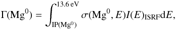 (3)σ(Mg0,E) is the photoionization cross section of neutral Mg for photon energies E above the ionization potential IP(Mg0) = 7.65 eV, and I(E)ISRF is the strength of the interstellar radiation field in the local neighborhood (expressed in photons cm-2 s-1 eV-1 integrated over 4πstr). The quantity C(Mg+,T) is the rate constant for the charge exchange reaction Mg0 + H+ → Mg+ + H0, and α(Mg+,T) is the sum of the radiative and dielectronic recombination rates for free electrons and ionized Mg at a temperature T. The equilibrium expressed in Eq. (2) should hold as long as the physical conditions do not change more rapidly than the e-folding time [α(Mg+,T)n(e) + Γ(Mg0) + C(Mg+,T)n(H+)] -1 ≈ 750 yr for changes in ratio of Mg0 to Mg+ (at T = 6000 K). In principle, a more comprehensive treatment should also include the effects of Mg ions being neutralized when they collide with dust grains (Weingartner & Draine 2001), but this effect is at most about 2% of recombination rate with free electrons under typical conditions that we consider: T ≈ 6000 K, n(e) ≈ 0.1 cm-3 and n(H0 + H+) ≈ 0.3 cm-3Gry & Jenkins (2014).
5.1.1. Far ultraviolet interstellar radiation field
In order to derive n(e) using Eq. (2), we must adopt a value for I(E)ISRF that appears in Eq. (3). There have been various estimates that have appeared in the literature for the strength of the ultraviolet photon flux in our location in the Galaxy, as summarized in Sect. 12.5 of Draine (2011). We have chosen to use the fluxes vs. wavelength defined by Mathis et al. (1983), which are depicted in Fig. 2 (black line in the upper left-hand corner).
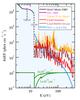 |
Fig. 2 Product of energy and fluxes of ionizing photons EeVI(E)ISRF as a function of energy EeV. Upper left: fluxes below the ionization potential of H at 13.6 eV, according to the model of Mathis et al. (1983). The energies that apply to the photoionization of neutral magnesium atoms are within the region bounded by the two vertical dashed lines. The short purple line depicts the observed fluxes discussed in Sect. 5.1.1. Lower colored traces: estimates for the unabsorbed local EUV and X-ray fluxes described in Sect. 6.1 that are responsible for ionizing neutral H, He, N, O, and Ar, along with the ions of C, S, Mg, Si, and Fe. The green lines at the bottom indicate the transmission factors for two values of the absorbing column densities of H I. |
We found that this radiation flux compares favorably with observations over a limited wavelength interval in the ultraviolet. For instance, we evaluated the sum of two components that have been observed to contribute to I(E)ISRF. One is the direct flux from stars at 1565 Å, where I(λ) = 1.21 × 10⁻⁶ erg cm-2 s-1 Å-1 = 9.53 × 10⁴ phot cm-2 s-1 Å-1 determined by Gondhalekar et al. (1980) from observations by the S2/68 Sky-survey telescope on the TD-1 satellite. The other is the diffuse field of photons arising from the scattering of starlight by dust I(λ) = 3.8 × 10⁴ phot cm-2 s-1 Å-1 over the interval 1370 to 1710 Å measured by Seon et al. (2011)5, who analyzed data from the SPEAR instrument on the Korean STSAT-1 satellite mission. The combination of these two fluxes is shown by the short purple line in Fig. 2, which is almost imperceptibly above the flux level in the same wavelength region in the model of Mathis et al. (1983).
5.1.2. Atomic data for magnesium
We adopted the photoionization cross sections σ(Mg0,E) calculated by Wang et al. (2010), who used a fully relativistic R-matrix method. These cross sections are in excellent agreement with the experimental results of Wehlitz et al. (2007). In our application of Eq. (3) to these cross sections and our adopted ISRF ionizing flux (Sect. 5.1.1), we found that Γ(Mg0) = 3.72 × 10⁻¹¹ s-16. Values for C(Mg+,T) have been calculated by Allan et al. (1988), and they have been expressed in parametric form by Kingdon & Ferland (1996). For example, C(Mg+,6000 K) = 5.3 × 10⁻¹¹ cm3 s-1. If the rate constant for the reaction Mg0 + He+ → Mg+ + He0 is greater than a few times 10-10 cm3 s-1, this mode of ionizing Mg could make a non-negligible shift in the equilibrium. Unfortunately, we were unable to find any determination (or even an estimate) for this rate in the literature. For the contribution of radiative recombination to α(Mg+,T), we adopted the analytic fit expressed by Badnell (2006). For the additional effect from dielectronic recombination, we used the determinations published by Altun et al. (2006). At T = 6000 K, α(Mg+,T) = 1.4 × 10⁻¹² cm3 s-1.
5.1.3. Deriving constraints
We equate n(Mg0) and n(Mg+) to our measurements of N(Mgi) and N(Mgii) and solve for n(e) by re-expressing Eq. (2) in the form, ![Mathematical equation: \begin{equation} \label{equilib3} n({\rm e})={\Gamma({\rm Mg}^0)\over \alpha({\rm Mg}^+,T)[N({\MgII})/N({\rm \MgI})]-C({\rm Mg}^+,T)/1.17}, \end{equation}](/articles/aa/full_html/2017/02/aa28987-16/aa28987-16-eq159.png) (4)where the factor 1.17 is an approximate value for n(e) /n(H+) (the extra electrons come from the ionization of helium).
(4)where the factor 1.17 is an approximate value for n(e) /n(H+) (the extra electrons come from the ionization of helium).
We recognize that the two column densities that appear in a quotient are subject to observational errors. A conventional approach for deriving the error of a quotient is to add in quadrature the relative errors of the two terms, yielding the relative error of the quotient. However, this scheme breaks down when the error in the denominator is not very much less than the denominator itself. For this reason, we resorted to a more robust way to derive the error of a quotient that has been developed by Geary (1930) for two independent quantities whose errors are normally distributed; for a concise description of this method see Appendix A of Jenkins (2009). We used this method here to define acceptable ± 1σ limits for the expression N(Mgii) /N(Mgi) in Eq. (4).
5.2. Fine-structure populations of ionized carbon atoms
The populations of the two fine-structure levels from the J-splitting of the ground state of C+, level1 =  and level2 =
  , are governed by several excitation and de-excitation processes, the most important of which are collisions with electrons with rate constants γ1,2(e,T) (upward) and γ2,1(e,T) (downward), which are balanced against spontaneous decays of the upper level radiating at λ = 157.6 μm with an Einstein A-coefficient A2,1 = 2.29 × 10⁻⁶ s-1Nussbaumer & Storey (1981). Additional channels which are small in comparison but not completely negligible include collisions with protons and neutral hydrogen atoms [rate constants γ1,2(H+,T) and γ1,2(H0,T) and their de-excitation counterparts] and optical pumping [rates r1,2(OP) and r2,1(OP)] by the ISRF acting on the two strong transitions out of the ground state at 1036 and 1335 Å. Balancing all rates, we find that
 ![Mathematical equation: \begin{eqnarray} \label{fsl_equilib} &&[n({\rm e})\gamma_{1,2}({\rm e},T) + n({\rm H}^+)\gamma_{1,2}({\rm H}^+,T)\nonumber\\ &&\quad+ n({\rm H}^0)\gamma_{1,2}({\rm H}^0,T) + r_{1,2}({\rm OP)}]n({\rm C}_{1/2}^+)=\nonumber\\ &&\quad[n({\rm e})\gamma_{2,1}({\rm e},T) + n({\rm H}^+)\gamma_{2,1}({\rm H}^+,T)\nonumber\\ &&\quad+ n({\rm H}^0)\gamma_{2,1}({\rm H}^0,T) + r_{2,1}({\rm OP})+A_{2,1}]n({\rm C}_{3/2}^+). \end{eqnarray}](/articles/aa/full_html/2017/02/aa28987-16/aa28987-16-eq178.png) (5)For the electron, proton and hydrogen rate constants, we know from the principle of detailed balance that
(5)For the electron, proton and hydrogen rate constants, we know from the principle of detailed balance that  (6)where g1 = 2, g2 = 4, and E/k = 91.2 K. The downward rate constant for electron collisions is given by
  (7)where we have adopted the collision strengths as a function of temperature Ω(e,T) from a fit by Draine (2011) to the results of Tayal (2008). Rates for excitations by protons γ1,2(H+,T) have been calculated by Bahcall & Wolf (1968) for T> 104 K; below this temperature such excitations are negligible compared to those caused by electrons. For γ2,1(H0,T) we used the analytic fit given by Barinovs et al. (2005), and once again we can use the principle of detailed balance to determine γ1,2(H0,T). We calculated that r1,2(OP) = 1.35 × 10⁻¹⁰ s-1 and r2,1(OP) is half as large. As stated earlier, we assumed that n(H+) ≈ n(e)/1.17 and n(H0) ≈ 0.2 cm-3; errors in these assumptions are not important because the effects of proton and hydrogen collisions are very small compared to those from electrons.
To solve for n(e) we rewrite Eq. (5) in the form ![Mathematical equation: \begin{eqnarray} \label{n(e)_solve} n({\rm e})&=&\Big\{ \left[n({\rm H}^0)\gamma_{2,1}({\rm H}^0,T) + r_{2,1}({\rm OP})+ A_{2,1}\right]\left[n({\rm C}_{3/2}^+)/n({\rm C}_{1/2}^+)\right]\nonumber\\ &&\quad- n({\rm H}^0)\gamma_{1,2}({\rm H}^0,T) - r_{1,2}({\rm OP})\Big\}\Big/\nonumber\\ &&\quad \Big\{\gamma_{1,2}({\rm e},T) + \gamma_{1,2}({\rm H}^+,T)/1.17\nonumber\\ &&\quad- \left[\gamma_{2,1}({\rm e},T) + \gamma_{2,1}({\rm H}^+,T)/1.17\right]\left[n({\rm C}_{3/2}^+)/n({\rm C}_{1/2}^+)\right]\Big\}. \end{eqnarray}](/articles/aa/full_html/2017/02/aa28987-16/aa28987-16-eq190.png) (8)Again, we used Geary’s (1930) method to evaluate the error in a quotient, in this case for
(8)Again, we used Geary’s (1930) method to evaluate the error in a quotient, in this case for  , as we had done earlier for N(Mg ii) /N(MgC i). We did not employ this scheme for sensing the uncertainty of the numerator over the denominator in Eq. (8) because the errors of the two are correlated instead of being independently random.
5.3. Combining the Mg and C constraints: results for n(e) and T
We can derive a unique combination of n(e) and T (and error limits thereof) by plotting the outcomes of Eqs. (4) and (8) on a diagram for these two quantities and finding the intersection of the two curves. The outcome is shown in Fig. 3 for the component at V = 8.8 km s-1 identified as the LIC. For this component we find T = 6000 K ±1000 K in very good agreement with the outcomes from the line fits, and n(e) = 0.13( + 0.04,−0.035) cm-3.
 |
Fig. 3 Allowed values for n(e) and T defined through the use of Eq. (4) for the observation of N(MgC i) /N(Mg ii) (solid green line) and Eq. (8) for N(C ii∗) /N(C ii) (solid red line) for the component identified as the LIC toward α Leo. Dashed line counterparts indicate the ± 1σ envelopes arising from errors in the column densities. The olive-colored fill indicates the region that satisfies both types of measurement within their 1σ uncertainties. |
Figure 4 shows the outcome for the sums of column densities of both velocity components. The use of the sum of column densities is justified since the column density distribution among both components does not vary much from species to species as shown in the last column of Table 1, which indicates that both components are likely to experience similar conditions. The closeness of the outcomes of Figs. 3 and 4 further validates this assumption. We find that for the sum of both components n(e) = 0.11( + 0.025,−0.03) cm-3. The preferred temperature of 6500 (+750, −600) K derived with the sum of column densities is slightly higher than the outcomes from the line fits, but T = 6000 K is still allowed within the 1σ error deviations7.
6. Ionization balance of other elements
Ultimately, we want to make an estimate for the density of neutral and ionized hydrogen by developing a model for the partial ionization of various atomic species and comparing the results with our observations. To solve for equilibrium ionization fractions, we must balance the ionization rates against the effects of radiative and dielectronic recombination with free electrons. Photons with energies above the ionization potential of hydrogen (13.6 eV) provide the principal means for governing the ionization balance between the preferred and next higher ionization stages of atoms under consideration. Charge exchange reactions also play a role in modifying the ionization balances. A representative ionization rate of a few 10-16 s-1 by cosmic rays (Indriolo & McCall 2012; Indriolo et al. 2015) is more than two orders of magnitude below our computed ionization rates by photons and thus can be ignored. The basic equations that one can use to evaluate the equilibrium concentrations of different ionization stages in a partially ionized medium have been outlined by Jenkins (2013)8. In the subsections that follow, we describe the properties of the principal parameters that we adopted for computing the equilibria.
6.1. Extreme Ultraviolet and X-ray radiation fields
For energies above 13.6 eV, nearly all of the Galactic direct and scattered radiation from stellar sources considered in Sect. 5.1.1 is blocked by the opacity of distant clouds of neutral hydrogen. For the special circumstances where this blockage is small, such as for nearby white dwarf stars or the B-type stars ϵ and β CMa, the local region can be exposed to energetic radiation (Craig et al. 1997), although it is much weaker than the fluxes at lower energies. The blue line in Fig. 2 shows a summation of fluxes from these sources at the Earth’s location computed by Vallerga (1998), after we have de-absorbed the radiation by multiplying it by exp [τ(H0,E)] for a representative column density N(H0) = 9 × 1017 cm-2 to the edge of the LIC (Wood et al. 2005; Gry & Jenkins 2014). Stars are the dominant source of ionizing radiation at energies just below the ionization potential of hydrogen, but their output falls below other radiation sources at higher energies.
Soft X-rays that could influence the local ionization are emitted by hot gases in three principal domains: (1) distant regions in the disk and halo of our Galaxy, characterized by the non-local emission defined by Kuntz & Snowden (2000), which they labeled as the trans-absorption emission (TAE); (2) emission from 106K gas in the Local Bubble; and (3) emission from an interface between the warm cloud and the surrounding hot medium (but see our conclusions in Sect. 7.5; perhaps this interface radiation is weaker). Jenkins (2013) has derived the fluxes at different energies for the distant X-ray background based on the description of TAE provided by Kuntz & Snowden (2000). These fluxes are shown by the orange trace in Fig. 2. Radiation levels from the hot gas in the Local Bubble and the LIC boundary have been estimated by Slavin & Frisch (2008; respectively shown as brown and red traces in the figure). However, Slavin & Frisch (2008) made no correction to the apparent Local Bubble emission to account for the fact that the soft X-ray background measurements were contaminated by the emission of X-rays caused by charge exchange when the solar wind interacts with exospheric hydrogen in the Earth’s magnetosheath and the heliospheric contribution arising from interactions with incoming interstellar neutral H and He. To correct for these two sources of emission, we have multiplied the apparent hot gas emission by a factor of 0.6 (Galeazzi et al. 2014; Snowden et al. 2014, 2015), which now serves as our estimate for the fraction of the observed diffuse flux that is produced by hot gas in the Local Bubble.
There are significant uncertainties in calculating the strength of the ionizing radiation for atoms and ions situated in the sight line toward α Leo. First, the unabsorbed flux intensities discussed earlier are approximate. Second, we assume that virtually all of the gas experiences the same amount of exposure to this radiation, i.e. we do not attempt to consider that some gas near the edge of the cloud is irradiated more strongly than that at the center. Finally, we describe the attenuation of this flux interior to our gas region in terms of a simple one-dimensional absorption law without considering any details of the complex (and unknown) geometry of the cloud or any full treatment of the three-dimensional radiative transfer. For the most part, errors that arise from neglecting these complications influence the outcome for what we designate as a representative absorbing column density, which itself is a free parameter that we adjust to give a satisfactory agreement between our calculations and the observed column densities. Also, our calculations of the influence of absorption in changing the ionization balance is important only for the elements H, N, O, and Ar, and has only a weak influence on C, S and Mg. The species Si and Fe remain almost entirely in the preferred singly ionized state, regardless of any reasonable changes in the radiation field strength.
For interstellar clouds with significantly higher self-shielding of the external radiation, the production of photons by internal sources, such as the chromospheric emissions by embedded late-type stars, can be relatively important. For our case with the sight line to α Leo, the shielding is so low that radiation from external sources completely overwhelms that from the internal ones9.
6.2. Secondary ionization processes
In the appendices of Jenkins (2013), there are descriptions of a number of secondary ionization processes that can in principle provide additional ionization routes that supplement the primary ones. However, owing to the fact that most of the ionizations are caused by photons with energies that are not far above 13.6 eV, the relative influence of these secondary processes is quite small. For instance, there are very few electrons produced by the photoionization of H0, He0, and He+ that have sufficient energy to create secondary ionizations of H0 and He0. The only non-primary modes that are not negligible in our case are the emissions of photons arising from the recombinations of He+ and He++ with electrons to produce He0 and He+. For instance, the rates ΓHe0(H0) and ΓHe+(H0) respectively represent 14% and 4% of the total H ionizations.
6.3. Atomic physics properties
6.3.1. Ionization cross sections
For H0 and He+, we use the cross sections described by Spitzer (1978). Cross sections for He0 and Ar0 are taken from Samson et al. (1994) and Marr & West (1976), respectively. Cross sections vs. energy for other neutral, singly and doubly ionized species are taken from the fitting formulae provided by Verner & Yakovlev (1995), which describe not only the cross sections for ionizing the outer electron, but also those for inner shell electrons by photons at higher energies.
6.3.2. Radiative and dielectronic recombination coefficients
Radiative recombinations to form H0 and He+ are taken from Spitzer (1978), and we used the radiative and dielectronic rates of Aldrovandi & Pequignot (1973) for the creation of He0. Recombinations to the lowest electronic level of H generate Lyman limit photons, most of which are absorbed within the region to ionize some other H atom. Thus, we excluded recombinations to this level by employing the Case B recombination coefficient Baker & Menzel (1938). Fitting formulae for the recombinations of other elements were taken from Shull & van Steenberg (1982), supplemented by rates to low lying levels of N0, N+, C+, C++ (Nussbaumer & Storey 1983) and Si+ (Nussbaumer & Storey 1986).
6.3.3. Charge exchange reaction rates
For computing the charge exchange rates with H0 for all elements except O, we used the fits specified by Kingdon & Ferland (1996). For those elements whose ionizations can be reduced by capturing an electron from He0 (but again excluding O), we evaluated rate constants for T = 6000 K by making logarithmic interpolations between the results for T = 103.5 and 104K given by Butler & Dalgarno (1980). Charge exchange rate constants for O+ reacting with H0 and He0 are respectively from Stancil et al. (1999) and Butler et al. (1980).
6.4. Column density of H I and H II
Our observation of the total column density of nitrogen, N(Ntot) = N(N i) + N(N ii) is our most secure way to estimate the total amount of neutral and ionized hydrogen in the sight line (our computed abundance of doubly ionized N should be very low, see Table 3 in Sect. 6.6). Generally, the depletion of nitrogen in the ISM is quite weak (−0.109 ± 0.119 dex), and it does not seem to vary when the depletions of other elements change (Jenkins 2009)10. We find that for the full line of sight, e.g. the sum of both velocity components, N(Htot) = 2.83 ( + 1.18,−0.69) × 1018 cm-2. Our specified error range for this column density includes the uncertainty in the sum of two observed nitrogen column densities and the uncertainty in the depletion, both of which are combined in quadrature. In this case we only consider the sum of the components since Copernicus data do not allow us to derive precise N ii column densities for each component separately.
For the partition of N(Htot) into the expected values of N(H0) and N(H+), we must rely chiefly on the observed nitrogen ionization fraction N(N i) /N(Ntot) = 0.60( + 0.042,−0.123) combined with our model for the photoionization of hydrogen. The most stringent way to confine the free parameters in this model is to force the outcome for n(e) to fall within the range of the observational result that we specified in Sect. 5.3. In making use of n(e), we acknowledge that it is driven by two quantities that are not measured explicitly: (1) the local volume density of hydrogen and (2) the amount of shielding of the external radiation by hydrogen and helium (as illustrated by the green traces in Fig. 2). By adjusting these two parameters, we can explore combinations that are consistent with our observed quantities, the nitrogen ionization fraction and n(e). Using this technique, we find that a representative local density n(Htot) = 0.30( + 0.10,−0.13) cm-3 gives a satisfactory fit, where the shielding of the external radiation could be within the range 4.3−7.0 × 1017 cm-2 of neutral hydrogen (and with n(He0) /n(H0) = 0.07)11. The model indicates that the neutral fractions of H range from 0.58 to 0.73.
Predicted column densities for the sum of both components.
Table 2 presents the outcomes for the expected column densities of H0 (along with other elements to be discussed later). The three columns that show such column densities present values that pertain to three combinations of n(Htot), n(e), and shielding column densities that gave acceptable results. For each column, the three rows labeled “Upper”, “Best”, and “Lower” indicate the values of N(H0) that are allowed within the uncertainties of N(Htot).
6.5. H I column density – a note of caution on the use of Lyman α to derive N(H I)
There is a large discrepancy between the apparent N(H i) derived from the Lyman α profile assuming the 2-component line-of-sight structure (N(H i) = 6.6 × 1018 cm-2) and the total N(H i) derived from the ionization model calculations (between 1.3 and 2.8 × 1018 cm-2, as shown in Table 2). Despite the high level of noise in the spectrum, Fig. 5 shows that the low column density from the model (red trace) does not produce a good fit to the data. On the other hand, as high a column density as 6.6 × 1018 cm-2 would imply the existence of extraordinarily large depletions for many metals, ones that are even higher than those that we discuss later (Sect. 6.6) and that approach the highest strengths of depletion in the Milky Way. This is a prospect that is very unlikely in such a diffuse gas.
 |
Fig. 5 Lyman α profile in the spectrum of α Leo. The original data have been smoothed by 20 pixels to reduce the apparent noise. The red trace shows the expected profile from the two warm components with a total N(H I)tot = 1.9 × 1018 cm-2 (as favoured by our model). The blue trace shows the profile when an extra component with T = 200 000 K and N(H i) = 2.1 × 1015 cm-2 is added to the fit (see Sect. 7.5). In all models an absorption of D i is included,with a fixed D/H ratio of 1.6 × 10⁻⁵. |
The danger of overestimating N(H i) from the Lyman α line when N(H i) is lower than about 1019 cm-2 had already been discussed by Vidal-Madjar & Ferlet (2002) and is supported further by the recognition by Wood et al. (2005) about the presence of extra absorption by hot gas from the heliosphere and/or an astrosphere around a number of target stars. Here the discrepancy may be due to the presence of very small amounts of high-velocity or high-temperature gas present in the line of sight and undetectable in the lines of other elements. This possibility is brought up again in Sect. 7.5 when we discuss the presence of interfaces with the hot gas.
Another interesting possibility is related to the claim by Gies et al. (2008) that α Leo has a previously undiscovered close companion, which may be a white dwarf star. Gies et al. (2008) suggest that although this companion should be much fainter than α Leo, it may contribute a non-negligible flux in the FUV and they note that “in fact, Morales et al. (2001) find that the spectral energy distribution of Regulus is about a factor of 2 brighter in the 1000−1200 Å range than predicted by model atmospheres for a single B7 V star”. In the context of this possibility, we conjecture that the Lyman-α absorption from the white dwarf atmosphere could be responsible for the extra absorption in the wings of the interstellar profile. However this hypothesis cannot be investigated any further because of the insufficient signal in the Lyman-α core, as well as the lack of information on the potential close companion, which has not yet been detected directly (Absil et al. 2011).
6.6. Predictions for the column densities of other elements
Logarithms of the predicted ion fractions.
Using the radiation fields and atomic data outlined in Sects. 6.1 to 6.3, we can compute the expected column densities for various atomic species that we were able to observe (other than N, which was used to predict the amount of H and its ionization fractions). In the first attempt to do this we assumed that their abundances equal the solar values relative to hydrogen and that their distribution of ion stages followed our ionization model. This revealed that lightly depleted species, such as C, O, and Ar, gave a good agreement with the observations, but elements that are known to be depleted in the ISM showed predicted values considerably above the observed ones.
We now investigate whether or not the pattern of depletions follows trends for different elements seen elsewhere in the local part of our Galaxy. In addition, we have a goal of understanding where the gas toward α Leo stands within the scale of severity of depletions. To accomplish these tasks, we make use of the parametric description developed by Jenkins (2009) that defines the depletions in terms of some constants that apply to each element and a variable known as F∗ for the overall strength of depletions from one location to the next. The elements S and Ar have undetermined or probably small depletions: we first assume zero depletions in our comparisons of computed column densities against observed ones, however these comparisons will evidence that a non-zero depletion is required for S (Sect. 7.7).
We have adjusted F∗ to give the least discrepancy between the calculated and observed abundances of the most depleted elements Mg, Si and Fe. After considering the combined errors (added in quadrature) in the observations, our determination of N(Htot), and the depletion constants for each element, we find that we have a good match with the observations for all elements except Mg when we specify a value of F∗ equal to 0.6. This value for F∗ seems extraordinarily high for a low density medium. Mg appears to be more strongly depleted than what we would expect for our most favorable F∗, as the upper error limit for the observed column density of Mg ii does not overlap any of the lower limits for the predictions for N(Mg+). Table 2 shows the outcomes for our models, which may be compared with the observations of the total column densities of both velocity components from the fourth column of Table 1.
7. Interpretation: implications for the properties of the local ISM
We have shown in the previous section that when combined with a comprehensive ionization model, our extensive collection of column densities for many different species in the direction of α Leo has offered a unique opportunity for us to develop a well constrained and internally consistent description for the state of the gas. This development enables us to surpass most previous analyses of the nearby interstellar material around the Sun.
7.1. Temperature
We have estimated temperatures by two independent methods. The first estimate of T directly results from the line profile analysis, as explained in Sect. 3.3, and as listed in Table 1. The second method is the analysis shown in Figs. 3 and 4, which combines constraints given by the ionization equilibrium of magnesium and the fine-structure populations of ionized carbon. We have applied the latter method considering first the two velocity components as a whole, and we find a gas temperature of 6500 ± 700 K. We also considered the column densities derived for the LIC component alone, and we find a somewhat broader temperature range, T = 6000 ± 1000 K. This temperature is in remarkable agreement with the temperature derived from the line profile analysis, T = 6000 ± 600 K.
Our temperature estimate is consistent with the weighted mean gas temperature derived by Redfield & Linsky (2004b) in the local warm clouds, found equal to 6680 K with a dispersion of 1490 K.
We note that it is similar although only marginally consistent with the temperature derived from IBEX outside the heliosphere (T ~ 7500 K; McComas et al. 2015). The difference may illustrate varying physical conditions within the LIC.
7.2. Densities
The electron density n(e) = 0.13( + 0.04,−0.035) cm-3 that we derive from Fig. 3 for the LIC alone is in excellent agreement with the range 0.125 ± 0.045 derived for the LIC in the direction to ϵ CMa by Gry & Jenkins (2001) as well as with the weighted mean value of n(e) = 0.12 ± 0.04 cm-3 derived in 7 lines of sight by Redfield & Falcon (2008).
The total hydrogen density n(Htot) = n(H0) + n(H+) derived from n(e) and the ionization fraction of N via our ionization model, is n(Htot) = 0.3( + 0.1,−0.13) cm-3.
The neutral hydrogen density then defined by the neutral fractions allowed within our model is n(H0) = 0.20 (+ 0.08, −0.10) cm-3. This value is in agreement with the value customarily cited in cloud modeling e.g. as in Slavin & Frisch (2008). It is also supported by the measurement of N(H i) toward AD Leo, 8.5° away in the sky from α Leo and only 4.7 pc away from the Sun. For AD Leo, Wood et al. (2005) reported log N(H i) = 18.47, which seems surprisingly high for such a nearby star. The implied average density over that sight line is n(H i) = 0.20 cm-3 which is the same as the preferred n(H i) derived from the ionization calculation for α Leo.
However, we note that this density contrasts with the mean value n(H i) = 0.053 cm-3 derived by GJ14 for the average of N(H i)/d in the four lines of sight in the N(H i) sample of Wood et al. (2005), where the presence of astrospheres around the target stars suggested that the sight lines are completely filled. We had noted that n(H i) varies in the LIC since the outcomes spanned values from 0.03 to 0.1 cm-3. Our new value for n(H i) in the line of sight toward α Leo, derived independently by a different method, is higher than all previous values and could be the evidence of an even larger n(H i) variation inside the LIC.
The total gas density n = n(Htot) + n(e) + n(He) = 0.44( + 0.13,−0.17) cm-3.
7.3. Pressure
The thermal pressure of the gas, calculated from T = 6500 ± 700 K and the above total gas density n, log (p/k) = 3.46( + 0.12,−0.22), is consistent with pressures found elsewhere in our part of the Galaxy, log (p/k) = 3.58 with an rms dispersion of 0.18 dex (Jenkins & Tripp 2011). This pressure is substantially higher than the turbulent pressure  (log (p/k) = 1.91), but it is considerably lower than that derived by Snowden et al. (2014) for the surrounding X-ray emitting hot gas, log (p/k) = 4.025(−0.046, + 0.42). This pressure difference between the two media might be reconciled by the support provided by a magnetic field within the LIC.
Zirnstein et al. (2016) derived from the observation of the IBEX ribbon a magnitude of B = 2.93 ± 0.08 μG for the local interstellar magnetic field far (1000 au) from the Sun. This magnetic field strength is equivalent to a pressure of only 2500 cm-3 K, which, if not stronger elsewhere, is insufficient to enable the LIC to withstand the pressure value for the surrounding hot gas. With Voyager I data however, Burlaga & Ness (2014) measured in 2013 a varying interstellar magnetic field of average 4.86 μG with a dispersion of 0.45 μG, which approaches the value ~5 μG needed to sustain a pressure balance with the hot gas. We revisit this issue in Sect. 7.5)
7.4. Filling factor
On the assumption that the gas has a uniform density in the region responsible for the two absorption components and a considerably lower density elsewhere, we find that the volume of the partially neutral gas that intercepts the sight line toward α Leo is small, i.e. we obtain a filling factor equal to N(H0)/ [n(H0)d] = 0.13( + 0.19,−0.04), where d = 24 pc. It follows that in this direction the extent of the partially neutral gas that includes the LIC is somewhere in the interval between 2.2 and 7.7 pc.
The remaining 16 to 22 pc is thus devoid of detectable amounts of neutral or partially neutral gas. The question is what fills the remaining space, which amounts to asking what fills the Local Bubble. Snowden et al. (2015) attribute 70 ± 22 RU (Rosat Units) of the ROSAT 1/4 kev emission detected in the direction to the LLCC to the emission of the hot bubble gas in the foreground to the cold cloud (after a correction of the ROSAT 1/4 kev data for the heliospheric and magnetosheath Solar Wind Charge eXchange (SWCX) emission). They interpret this emission as occurring over a path length of 29 ± 11 pc in the Local Bubble plasma, made of gas at T = 1.18 ± 0.01 × 10⁶ K and n(e) = 4.68 ± 0.47 × 10⁻³ cm-3 (Snowden et al. 2014). If this hot, soft X-ray emitting, gas fills most of the line of sight to the LLCC, it is more than probable that it also fills a large fraction of the line of sight to α Leo, which is only 4° away.
We can note therefore that the star α Leo at a distance of 24 pc is very likely to be surrounded by hot gas. We have no evidence that it is embedded in partially neutral gas and therefore we do not expect it to exhibit an astrosphere. Thus the extra absorption in the Lyman-α line cannot be explained by the presence of an astrosphere around α Leo.
7.5. Attempted detection of the warm/hot gas interface
It follows from the foregoing section that the nearest portion of the line of sight from the Sun to α Leo has about 5 pc of warm diffuse gas, and about 19 pc of hot plasma. This implies that the line of sight crosses at least once the outer edge of the cloud. In the contact zone between the cloud warm gas and the hot gas two fundamental kinds of interactions may occur: one is a conduction front, which, depending on the age of the interface, may be a conduit for either evaporation of the warm gas into the hot gas or the condensation of the hot gas onto the cooler material (Ballet et al. 1986; Boehringer & Hartquist 1987; Slavin 1989; Borkowski et al. 1990). The second kind of interaction is a turbulent mixing layer that arises when the cool medium is moving relative to the hot gas and, as a result of instabilities, becomes entrained and mixed into the hot, more diffuse gas. Models for these turbulent mixing layers were initially proposed by Begelman & Fabian (1990) and further developed by Slavin et al. (1993) and Kwak & Shelton (2010). Both types of interaction create regions of intermediate temperature that contain highly ionized metals, and all models predict substantial column densities for C iv, N v, Si iv and O vi.
Our STIS spectrum of α Leo shows no evidence for any of the high ion species – see the upper limits in Table 1. Snowden et al. (2015) also report the absence of a manifestation of an interface between the cold LLCC gas and the hot Local Bubble gas since the X-ray data show no limb brightening at the edge of the LLCC (although they concede that such emission could occur at energies below the Rosat 1/4 keV passband).
Thermal conduction between the hot and warm media occurs primarily along magnetic field lines, and the electron heat flux is governed by the temperature gradient along such lines (Balbus 1986). Borkowski et al. (1990) showed that in a magnetized thermal conduction front, the predicted ion column densities vary with time, but more importantly, they can change by more than an order of magnitude depending on the inclination of the magnetic field relative to the front in the hot gas θh0. We now address the issue of the possible influence of a magnetic field on the hot to warm interface in front of α Leo.
Zirnstein et al. (2016) found that the magnetic field at about 1000 AU from the Sun was oriented toward 227.28° ± 0.69°, 34.62° ± 0.45° in ecliptic longitude and latitude. We convert this to ℓ ~ 26.1° and b ~ 49.5° in Galactic coordinates. This means that in the direction to α Leo, the magnetic field makes an angle of 79 ° with respect to the direction of α Leo, i.e. it is almost perpendicular to the line of sight.
We have no explicit knowledge about the orientation of the interface’s normal relative to our sight line, but if the angle between them is not very large, the field direction may be nearly parallel to the front. Moreover, this field is strongly coupled to the partly ionized warm medium and thus is probably influenced by forces on the gas near the front. It therefore follows that the field may be strengthened and pushed into closer alignment with the surface of the front if it is compressed so that it can brace the LIC to withstand the extra pressure from the hot medium (recall that the thermal pressure of the hot medium is probably larger than that of the LIC). This configuration could steepen the temperature gradient across the front.
Figure 6 of Borkowski et al. (1990) shows that for θh0 = 0° the column density predictions for C iv (in log from 12.6 to 12.05) are above our detection limits for a front younger than 106yr, however when θh0 = 60° or 85° the predicted column densities are below our detection limits for all ions. Therefore in the case where the hot gas magnetic field runs almost parallel to the cloud edge, which may be the case for the direction to α Leo, the interface high ion column densities could be reduced to the point that they are not detectable by our observations.
The H i profile however indicates that an extra absorption is present that cannot be reconciled with our analysis of the low-ionization species (Sect. 6.5). The contributions from hot gas have already been invoked to interpret Lyman α profiles in low-column lines of sight, such as ϵ CMa (Gry et al. 1995), Sirius A (Hébrard et al. 1999) and the astrospheres stars (Wood et al. 2005).
Let us first estimate the contribution of the Hot-Bubble gas to the profile. If this gas along the line of sight has the characteristics described by Snowden et al. (2014) over the path length discussed in Sect. 7.4 (~19 pc), we estimate a total H column density of 2.7 × 1017 cm-2. Under collisional ionization equilibrium (CIE) conditions, the neutral fraction expected in a gas at T ~ 1.2 × 10⁶ is equal to 1.9 × 10⁻⁷ (Gnat & Sternberg 2007) (calculated from the on-line tool provided by O. Gnat), yielding a neutral H column density of 5.1 × 1010 cm-2. At this temperature the b-value is 140 km s-1, which results in a profile width of FWHM = 0.95 Å that is compatible with the observed profile width (see Fig. 5), but the column density that we computed produces a central optical depth of only 2.8 × 10⁻⁴. The neutral hydrogen present amid the hot gas of the Local Bubble should therefore be undetectable in the Lyman α profile.
Alternatively, we may consider that the extra H i absorption arises from the interface between the cloud and the hot gas. At a typical interface temperature of 2 × 10⁵ K, the H i column density needed to produce the missing absorption in the Lyman profile is N(H i) = 2.1 × 1015 cm-2 (shown in Fig. 5). If the gas were in CIE, this would imply a total column density of 3.3 × 1020 cm-2, which is unrealistically high in view of the total column density of the cloud itself. A more promising approach may be to consider the possibility that in the interface between the warm and hot phases, the collisional ionization of the hydrogen lags behind that expected for CIE as the temperature increases within the evaporation flow (Ballet et al. 1986). In such a circumstance, the required total amount of hydrogen would be considerably less. We are not aware of explicit calculations discussed in the literature for the non-equilibrium expectations for N(H I) in such flows at the level of thermal pressures that apply to our case. It might be the case that the extra H I absorption at large displacements from the line core could be a more sensitive indicator of an interface than any evidence provided by the highly ionized metal species.
7.6. Cloud ionization
The neutral hydrogen density of n(H0) = 0.20 (+0.08, −0.1) cm-3 and the ionized hydrogen density of n(H+) = 0.10 (+0.02, −0.03) cm-3 lead to an ionization fraction of one third, χ = 0.33(+0.09, −0.06).
A notable outcome of our ionization model is that the shielding column densities are substantially lower than half of N(H0). This can plausibly be explained by the geometry of the LIC, which we propose is thinner in the Canis Majoris direction. Supporting this idea is the fact that toward the star ϵ CMa, a powerful source of ionization of the local medium, the total O i and N i column densities are only 25% of those toward α Leo (Gry & Jenkins 2001). From this we infer a total neutral gas column density of N(H i) ~5 × 1017 cm-2 toward the ionizing source ϵ CMa, including about ~3.5 × 1017 cm-2 for the LIC alone. Since α Leo is only 61° from ϵ CMa, and since the neutral gas subtends only a short distance, it is not difficult to imagine that the line of sight to α Leo runs not far from the border on the exposed side of the LIC for most of the cloud length, explaining the low shielding column density.
Table 3 indicates for our preferred ionization condition how different elements are distributed among different ionization levels that are relevant. The elements Si, S, and Fe have ion fractions near unity for their preferred stages of ionization, and this outcome holds for all acceptable ionization conditions. The elements C, N, O, Mg, and Ar have some concentrations in higher levels, and these fractions can vary within our most acceptable combinations of n(e) and n(Htot).
We note that He is always more ionized than H. The neutral fractions for He range from 0.42 to 0.57 while those for H range from 0.58 to 0.73. Our calculated ratio n(He0) /n(H0) varies from 0.064 for [n(e),n(Htot)] = [0.08,0.25] to 0.093 for [n(e),n(Htot)] = [0.135,0.30]. These values for the neutral helium to hydrogen ratios are consistent with the findings for various local lines of sight considered by Dupuis et al. (1995) and Barstow et al. (1997).
Our computed outcomes for the abundances of highly ionized species are lower than what was calculated by Slavin & Frisch (2008, model 26). This difference may be explained in part by their using a higher soft X-ray radiation field since they did not reduce the soft X-ray flux estimate for the contamination by a contribution from the solar wind charge exchange.
7.7. Depletion
As we indicated in Sect. 6.6, we find a substantial metal depletion in the line of sight toward α Leo, consistent for all elements with a line of sight depletion strength F∗ = 0.6 (following the scale established by Jenkins 2009), except for magnesium which is even more depleted. The fact that depletions are present in our environment comes as no surprise, as this behavior has been noted elsewhere in the local ISM (Wood et al. 2002; Slavin & Frisch 2007; Frisch et al. 2011; Gry & Jenkins 2014; Kimura et al. 2003; Kimura 2015). The fact that magnesium is over-depleted relative to other elements was already noticed by GJ14 for the bulk of sight-lines through the LIC. This may be relevant to a particular change in the composition of dust in the solar neighborhood.
Logarithms of elemental abundances and depletion values.
Table 4 lists the measured abundances of all observed species relative to the total hydrogen, after corrections for unseen ionization stages using the ionization fractions calculated in the model and given in Table 3. In calculating the depletions, we maintain consistency with Jenkins (2009) by using as a comparison the recommended proto-solar abundance values by Lodders (2003), i.e. the values of A(El)0 listed in her Table 2. The newer abundances by Lodders & Palme (2009) differ by only ±0.02 dex from those we used, except for Ar (−0.07 dex) and S (−0.05 dex).
For most studies of interstellar abundances, measurements of N(Al ii) are difficult because the Al ii absorption feature at 1671 Å is usually highly saturated. However, observations over short paths in low density media avoid this problem and provide special opportunities to measure the depletion of aluminum in the gas phase. For the spectrum of α Leo, our measurement of N(Al ii) from the unsaturated absorption feature and the upper limit on N(Al iii), combined with our estimate of N(Htot), yield an aluminum abundance of log(N(Al)/N(H)) = −7.00 ± 0.18. Compared to the solar abundance of aluminum [log(Al/H)⊙ = −5.46 ± 0.02 from Lodders (2003), we derive a depletion of [Al/H] = −1.54 ± 0.18. In the line of sight to α Leo aluminum is significantly depleted in the gas phase with a depletion value similar to that of iron (−1.60 dex).
It is noteworthy that our depletions for certain elements seem to be larger than typical values in the local region. For instance, we find that log N(Si II) /N(O I) = −1.95 for α Leo is surpassed by only 4 out of 32 sight lines studied by Redfield & Linsky (2004a). Likewise, our determination log N(Al II) /N(O I) = −3.61 represents a depletion of Al that is matched or exceeded by only 2 out of 17 cases examined in this same investigation, not counting upper limits that were weaker (i.e. larger) than our result. GJ14 had noted the existence of an abundance gradient for Fe and Mg within the LIC, with their depletions increasing along the direction of motion from the rear to the front of the cloud. Although the angle between the direction of motion and the direction of α Leo is 76°, placing this sight line in the middle zone with intermediate depletion, the Mg and Fe depletion values found toward α Leo are consistent with the highest depletions12, found by GJ14 in the head of the cloud. In the direction toward Capella (20° from the head of the cloud) Wood et al. (2002) have derived depletion values in the LIC for all our elements but argon and sulfur. All values are compatible with our findings and the agreement is excellent for Mg, as well as for Al and Si.
Our derived depletion strength F∗ = 0.6 (Sect. 6.6) is higher than any of the synthetic F∗ values13 found by Jenkins (2009) for WD stars in the Local Bubble with an average value of F∗ sync = 0.15 ± 0.23. These stars are generally more distant than α Leo, but they give the general trend for sight lines that penetrate other low density clouds in the Local Bubble. However, Jenkins (2009) notes that six of the stars have F∗ sync ≥ 0.3, indicating that moderately strong depletions do exist in our general vicinity.
We note that both oxygen and argon appear to be undepleted in the gas phase.
Sulfur, by contrast, shows a depletion by almost a factor of two. Sulfur has often been considered to be undepleted, and as such has been used in many studies as a standard for zero depletion. Jenkins (2009) presented some evidence for S depletion but noted that S is a troublesome element because N(S ii) usually cannot be reliably measured except for cases where column densities are low. Furthermore because of its high ionization potential (23 eV), some of the S ii can arise from the H II region around the target star. The line of sight toward α Leo, where the S ii lines are not saturated and the total H column density is known, provides an important indication that sulfur can indeed be depleted in the ISM.
Carbon may be slightly overabundant, although its overabundance is not significant after considering the error bars on N(C II). An overabundance of carbon in the local ISM had already been proposed by Slavin & Frisch (2006). We find toward α Leo a gas-phase abundance close to their lower limit of 330 ppm. We confirm here their finding that the carbon to sulfur ratio is higher than solar, with C/S = 34 (+13, −6), to be compared with the solar ratio of 16. However toward α Leo this indicates sulfur depletion rather than an overabundance of carbon.
7.8. Secondary components
While our ionization analysis applies to all of the matter present in the line of sight, we recognize that the gas is distributed between two distinct velocity components separated by 5.6 km s-1. The dominant component is the LIC with ≈75% of the total column density. As mentioned in Sect. 4, the second component is at a positive shift relative to the LIC. This behavior is consistent with that of other secondary components in this region of the sky, as shown in Fig. 6, which is an update of Fig. 12 of GJ14.
 |
Fig. 6 Map of all secondary components, showing their velocity shift relative to the LIC component. This plot is the same as Fig. 12 of Gry & Jenkins (2014), but with one correction and a few additions including α Leo. Black asterisks signal the position of all targets. Blue/red squares mark secondary components with negative/positive shifts, and the size of the symbols scales with the amplitude of the shift. Dark blue symbols indicate the components having a uniform velocity shift of −7.2 ± 1.5km s-1 relative to the LIC (i.e. the Cetus Ripple); light blue symbols represent the other blue-shifted components. The blue circle at l = 2.3°, b = 31.4° shows the “Warm Breeze” heliospheric inflow direction. |
In GJ14 we had shown that a secondary component moving toward the cloud center with a relative velocity close to −7 km s-1 was present in all sight-lines on half of the sky (shown in dark blue in Fig. 6). We called this component the Cetus Ripple in view of the rough location in the sky of its center, and we showed that all observed characteristics were consistent with a shock travelling in the LIC toward the cloud interior at a velocity of 20 to 26 km s-1. On the other side of the sky, where α Leo is located, all secondary components have a positive velocity shift relative to the LIC, meaning that they move away from it or that they move outwards if they are included in the cloud.
As shown in the last column of Table 1 the proportion of gas at the LIC velocity versus the proportion of gas in the second component is very stable from species to species, which indicates similar conditions in both components. This makes it plausible that the second component is but an inclusion within the LIC.
This second component, along with other secondary components seen in the direction of the nearest stars, may be related to kinematic disturbances within the local cloud. They may represent internal flows of matter with different velocities in the form of waves propagating in the local cloud matter.
In this context, we may try to establish a connection with the IBEX “Warm Breeze”, a second component of neutral He discovered in the IBEX data, with inflow Galactic coordinates ℓ = 2.3°,b = 31.4°, with a different velocity, temperature and density than the main component that corresponds to the LIC flowing into the heliosphere. Kubiak et al. (2014) who report its discovery offer several possible interpretations involving heliospheric configurations, and they also propose that the Warm Breeze might be a flow of interstellar matter not thermalized with the LIC material, moving in the LIC with a relative velocity equal to VWB − VLIC = 13.6km s-1. Although our secondary components are in principle more extended than the IBEX Warm Breeze (they represent a substantial portion of the matter on most lines of sight even if the LIC is the dominant component), the Warm Breeze could be the local signature of an interstellar component of the same nature as the secondary components present in many stellar lines of sight.
8. Implications for the Local Leo Cold Cloud (LLCC)
Results discussed in the previous sections show that the interstellar absorption features detected in the line of sight toward α Leo are fully consistent in both velocity and magnitude with what we expect from the local ISM. There is no evidence for the presence of cold and dense gas of the type seen in the interior of the LLCC, and also no evidence for an excess of warm diffuse gas.
The good coincidence in velocity between the LIC in this direction and the LLCC is however worth pointing out. By performing a least-square fit to the velocities measured in the main body of the LLCC, Peek et al (2011) predicted an LSR velocity of 3.19 km s-1 at the position of α Leo for the LLCC assuming that it is moving as a solid body. This velocity translates to a heliocentric velocity of 9.3 km s-1, which is in excellent agreement with GJ14 prediction for the LIC velocity. The coincidence is even more compelling when we notice that it holds true along the long string of dense clouds (Haud 2010) that stretches across 80° in the sky and that includes the LLCC. Along this string the GJ14 model for the deformed LIC predicts LSR velocities from 0 km s-1 to 12.7 km s-1 from its northern location around (ℓ,b) = (240°, + 46°) to its south-western end around (180°, 20°). This is in intriguingly good agreement with the color-coded cold matter velocities displayed all along the string in Fig. 2a of Haud (2010)
The weak Ca ii absorption feature in the optical spectrum of α Leo studied in detail by Peek et al. (2011), is detected at an LSR velocity of 3.1 km s-1. Since it is identical to the LLCC velocity, Peek et al. (2011) claimed that the Ca II absorption feature arises from the outermost portions of the LLCC extending across the α Leo line of sight. This interpretation is however challenged by the coincidence of this feature with the properties of the LIC found by us and other investigators, as we discuss below.
The LSR velocity quoted by Peek et al. (2011), which we convert to a heliocentric velocity of +9.2 km s-1, coincides with that of our Component 1 and the GJ14 prediction of the LIC velocity. Frisch et al. (2002) refer to a Ca II spectrum taken with a resolution of about 1.3 km s-1, and with a signal-to-noise ratio of about 500. A fit to the normalized line profile as a single component yielded (D. Welty, priv. comm.) b ~ 3.6 ± 0.7km s-1, and vhel ~ 10.5 ± 0.5 km s-1, which are values that are consistent with our two-component model for α Leo, if expressed in just the context of a single component. Futhermore the derived column density is N(Ca ii) ~ 5.0 ± 0.8 × 109 cm-2, which is generally typical of values found for the LIC (Lallement & Bertin 1992). For example, it is identical to the Ca ii column densities listed for the LIC toward α Aql (5.1 pc, N(CaII) ~ 7 × 109 cm-2, Ferlet et al. 1986) or δ Cas (30.5 pc, N(Ca II) = 5.0 ± 2.5 × 109 cm-2, Lallement & Bertin 1992), which both show Mg ii column densities very close to those we find for α Leo (Lallement et al. 1996; Lallement & Ferlet 1997).
We conclude that the Ca ii feature is consistent with being produced in the LIC. Now, if this feature is not attributed to the LLCC, there is no evidence that the LLCC must be located in front of α Leo (as had been proposed by Peek et al. 2011). It follows that the distance to α Leo (24 pc) no longer represents a reliable upper limit for the distance to the LLCC. The only firm upper limit to the distance of the cloud therefore remains at 45 pc, as established by Meyer et al. (2006).
This has an important implication regarding the understanding of the hot gas observed in the Local Bubble. Snowden et al. (2015) showed that the soft X-ray foreground emission to the LLCC “is only marginally consistent with the range of possible LHB plasma path lengths between the LLCC and the LIC”. This conclusion was drawn by adopting 24 pc as upper limit to the LLCC distance. Since we have now shown that this upper limit is no longer warranted, the constraint is much less stringent, and there is room for their required path length DLHB = 29 ± 11 pc for the hot gas in front of the LLCC.
With the observation of the hot gas foreground emission occurring over a length of 29 ± 11 pc (Snowden et al. 2015) we obtain a very consistent picture where the warm, diffuse, partially neutral, gas extends out for a total of 3( + 5,−1) pc complemented by 29 ± 11 pc of hot gas, until it reaches the cold dense matter of the LLCC at a distance of 33.5 ± 11.3 pc. This maximum distance derived from the path length of the soft X-ray emission is now fully consistent with the LLCC distance upper limit derived from the absorption spectra of background stars.
Comparing the path length derived for the warm diffuse gas observed in the α Leo line of sight (between 2 and 8 pc for the sum of our two components) to the minimum distance of the LLCC of 11 pc Peek et al. (2011), we could conclude that it is likely that the two clouds are not physically contiguous, if the LIC is supposed to be a continuous medium.
Yet, the excellent kinematical coincidences also lead us to put forward the hypothesis that the LLCC, as well as the Haud ring, are part of a complex of gas that may somehow be physically related to the LIC. In the picture of the LIC being a continuous medium, we recognize that the LLCC and the LIC seem to be separated by a long path of hot gas. However in the hypotheses of a patchy cloud, the low filling factor could also be interpreted as the presence of voids within the volume of the LIC, the LIC presenting a “Swiss cheese” structure or a filamentary structure, warm gas filaments alternating with voids filled with hot gas. In this case, the overall volume occupied by the diffuse local cloud would reach further out, out to the distance of the LLCC. In this hypothesis the LIC could spatially coincide with outer regions of the LLCC, or the LLCC could be a clump of cold dense gas formed inside the diffuse warm gas of the LIC.
9. Summary and conclusion
We have analyzed the ultraviolet absorption spectrum of the nearby star α Leo to characterize the interstellar medium in its line of sight, and in particular the warm diffuse interstellar cloud surrounding the Sun.
-
The strongest of the two velocity components coincides with thepredictions for the LIC detected in all directions around the Sun,according to the picture proposed by Gry & Jenkins (2014). Thesecond, smaller, component exhibits a velocity shift of+5.4 km s-1 relative to themain component, in agreement with shifts observed in other linesof sight in this region of the sky.
-
By performing profile fitting on the spectra, we derive column density intervals or upper limits for 18 atoms or ions (Table 1). The LIC contains about 75% of the total matter in the line of sight and the distribution between both components does not vary significantly from element to element.
-
The temperature T and the electron density n(e) are derived by combining the measurements of the fine-structure level excitation of C ii and the ionization equilibrium of Mg i and Mg ii.
-
After estimating the local interstellar radiation field in the UV, extreme UV, and X-ray domains (Fig. 2) and considering all possible ionizing and recombination processes, we study the ionization balance of all elements and create a model that describes consistently the partial ionization of the gas. Two free parameters in this model are (1) the amount of shielding of this radiation by neutral hydrogen and helium and (2) the volume density of hydrogen.
-
The total (neutral plus ionized) amount of hydrogen N(Htot) is derived from the sum of the N i and N ii column densities.
-
The densities of neutral and ionized hydrogen, and hence N(H i), result from our model for the photoionization of hydrogen and our knowledge of n(e).
-
The ionization fractions of all elements follow from our model (Table 3), and their comparisons with the observations provide a measure of the depletion of metals in the gas phase.
-
Table 5 summarizes the characteristics derived from this analysis for the warm interstellar matter in the α Leo sight line.
Table 5Characteristics of the warm interstellar gas in the line of sight of α Leo.
With the exception of the temperatures and the electron densities that we derived for each of the velocity components, the analysis has been done for the combination of the two components. Nevertheless since we have shown that the conditions in both components are likely to be identical, the densities and the ionization ratios found for them are likely to apply to just the LIC alone.
-
From the neutral hydrogen column and volume densities we derive a filling factor of only 13% for the warm gas, the remaining space is probably filled with hot, soft-X-ray emitting gas, in agreement with measurements of the diffuse soft X-ray background radiation.
-
We do not detect any absorption features in the highly ionized species that could be produced in the interfaces between the warm clouds and the surrounding hot gas, possibly because of the reduction of thermal conduction due to the alignment of the magnetic field with the surface of the conduction front. On the other hand, an extra component of hot neutral hydrogen, required to fit the Lyman α absorption feature, may turn out to be the best interface signature.
-
This sight-line is particularly interesting because it is close to a nearby cold cloud called the Local Leo Cold Cloud (LLCC) discovered by Meyer et al. (2006). We show that the Ca II absorption that had been invoked to set a new upper limit of 24 pc for the distance of LLCC is actually fully consistent with just the LIC absorption. Therefore, the LLCC upper limit remains 45 pc and this reconciles the LLCC distance with the estimated path length of the measured X-ray emission from the foreground hot gas in the Local Bubble, which places the LLCC at a distance of 33.5 ± 11.3 pc.
-
We note the remarkable velocity coincidence between the LIC and the LLCC. We also note that in the hypothesis that the LIC has a patchy structure, with diffuse warm gas alternating with hot gas along the line of sight, the LIC could reach as far as the distance of the LLCC and the two clouds may be physically related.
We are unable to correct for rotation of the Earth’s atmosphere. For the declination of α Leo (12°) the telluric features can experience a shift as large as 0.45 km s-1 when viewed at large zenith angles.
The Copernicus observations of the Fe ii lines were carried out using either the V1 or V2 detectors, both of which had seriously compromised photometric precision caused by extraordinarily large backgrounds arising from charged particle radiation interacting with the photomultiplier entrance windows Rogerson et al. (1973a).
A note on nomenclature: in the present article, we retain the designation local interstellar cloud (LIC) for the medium surrounding the Sun, which is a convention followed by many authors in the past. However, we envision that it refers to a single, coherent medium defined by GJ14 that accounts for most of the matter out to a distance of many tens of pc. This term is not to be confused with a narrower definition of the LIC proposed by Redfield & Linsky (2008), who declared that the nearby gas is broken into many distinct clouds, one of which they called the LIC.
This model proposes a mean velocity vector of magnitude V = 25.53 km s-1 pointing toward the Galactic coordinates l = 185.84°; b = −12.79°, which is nearly identical to the flow that is impacting the heliosphere (Möbius et al. 2004; McComas et al. 2012). The model also includes deviations from the mean vector to account for the cloud deceleration and deformation.
We avoided using the average fluxes from direct starlight measured by Seon et al. (2011) because their sky coverage omitted regions that contained particularly bright stars: e.g. one may compare Fig. 1 of Seon et al. (2011) with Fig. 1 of Gondhalekar et al. (1980; but noting that one depiction is inverted horizontally with respect to the other).
This ionization rate is lower than those adopted by Gry & Jenkins (2001) and Slavin & Frisch (2006), which equaled 6.1 and 4.5 × 10⁻¹¹ s-1, respectively. The former used the radiation field of Mathis et al. (1983), while the latter adopted the (stellar plus diffuse) field of Gondhalekar et al. (1980). Both authors used values of σ(Mg0,E) from the parametric description of Verner et al. (1996), which is higher than the cross sections of Wang et al. (2010) at photon energies between the IP(Mg0) and 10.5 eV.
The relevant equations in Jenkins (2013) are those given in Sects. 6.4 and 6.5 of that paper, which apply to elements that have appreciable amounts of their atoms in neutral form. For the equilibrium of any predominantly singly ionized element X, the fractions f0(X,T), f+(X,T) and f++(X,T) can be evaluated using the same equations and rates for the higher stages of ionization, except that these three fractions then apply to the concentrations of X+, X++, and X3+, respectively.
While some white dwarfs are inside the LIC, their radiations are included in the sum of white dwarf fluxes compiled by Vallerga (1998).
Any uncertainty in the reference (solar) abundance adopted by Jenkins (2009) should not affect our inferred factor to multiply N(Ntot) to get N(Htot) since changes of opposite sign would be reflected in the derived amount of depletion.
The largest value expressed here does not appear in Table 2 because it pertains to [n(e),n(Htot)] = [0.08,0.25], which is not an acceptable combination.
The GJ14 depletion values for Fe should be increased by −0.17 to account for the ionization of H. No such correction is needed for Mg, since the ionization fraction of Mg ii is similar to that of H i in our model.
A synthetic F∗ is a depletion outcome that is based solely on the relative abundances of various elements, without reference to the amount of hydrogen present.
Acknowledgments
Based on observations made with the NASA/ESA Hubble Space Telescope that were obtained for the ASTRAL Treasury program during the Cycle 21 observing session. Support for the research by E.B.J. was provided by NASA through a grant HST-GO-13346.15-A to Princeton University from the Space Telescope Science Institute (STScI), which is operated by the Association of Universities for Research in Astronomy, Inc. under the NASA contract NAS 5-26555. The Copernicus data were obtained from the Mikulski Archive for Space Telescopes (MAST) at STScI, supported by the NASA Office of Space Science via grant NNX09AF08G and by other grants and contracts. E.B.J. is grateful to Aix-Marseille Université for providing a visitor grant to support his 1-month visit to LAM where this research was initiated. We are thankful to T. Ayres for his dedication and skill in organizing and programming the observations that made up the Hot Stars episode of the ASTRAL program.
References
- Absil, O., Le Bouquin, J.-B., Berger, J.-P., et al. 2011, A&A, 535, A68 [NASA ADS] [CrossRef] [EDP Sciences] [Google Scholar]
- Aldrovandi, S. M. V., & Pequignot, D. 1973, A&A, 25, 137 [NASA ADS] [Google Scholar]
- Allan, R. J., Clegg, R. E. S., Dickinson, A. S., & Flower, D. R. 1988, MNRAS, 235, 1245 [NASA ADS] [CrossRef] [Google Scholar]
- Altun, Z., Yumak, A., Badnell, N. R., Loch, S. D., & Pindzola, M. S. 2006, A&A, 447, 1165 [NASA ADS] [CrossRef] [EDP Sciences] [Google Scholar]
- Badnell, N. R. 2006, ApJS, 167, 334 [NASA ADS] [CrossRef] [Google Scholar]
- Bahcall, J. N., & Wolf, R. A. 1968, ApJ, 152, 701 [NASA ADS] [CrossRef] [Google Scholar]
- Baker, J. G., & Menzel, D. H. 1938, ApJ, 88, 52 [NASA ADS] [CrossRef] [Google Scholar]
- Balbus, S. A. 1986, ApJ, 304, 787 [NASA ADS] [CrossRef] [Google Scholar]
- Ballet, J., Arnaud, M., & Rothenflug, R. 1986, A&A, 161, 12 [NASA ADS] [Google Scholar]
- Barinovs, Ğ., van Hemert, M. C., Krems, R., & Dalgarno, A. 2005, ApJ, 620, 537 [NASA ADS] [CrossRef] [Google Scholar]
- Barstow, M. A., Dobbie, P. D., Holberg, J. B., Hubeny, I., & Lanz, T. 1997, MNRAS, 286, 58 [NASA ADS] [CrossRef] [Google Scholar]
- Barstow, M. A., Good, S. A., Holberg, J. B., et al. 2003, MNRAS, 341, 870 [NASA ADS] [CrossRef] [Google Scholar]
- Barstow, M. A., Boyce, D. D., Welsh, B. Y., et al. 2010, ApJ, 723, 1762 [NASA ADS] [CrossRef] [Google Scholar]
- Barstow, M. A., Barstow, J. K., Casewell, S. L., Holberg, J. B., & Hubeny, I. 2014, MNRAS, 440, 1607 [NASA ADS] [CrossRef] [Google Scholar]
- Begelman, M. C., & Fabian, A. C. 1990, MNRAS, 244, 26 [Google Scholar]
- Begum, A., Stanimirović, S., Peek, J. E., et al. 2010, ApJ, 722, 395 [NASA ADS] [CrossRef] [Google Scholar]
- Boehringer, H., & Hartquist, T. W. 1987, MNRAS, 228, 915 [NASA ADS] [CrossRef] [Google Scholar]
- Bohlin, R. C. 1975, ApJ, 200, 402 [NASA ADS] [CrossRef] [Google Scholar]
- Borkowski, K. J., Balbus, S. A., & Fristrom, C. C. 1990, ApJ, 355, 501 [NASA ADS] [CrossRef] [Google Scholar]
- Burlaga, L. F., & Ness, N. F. 2014, ApJ, 795, L19 [NASA ADS] [CrossRef] [Google Scholar]
- Butler, S. E., & Dalgarno, A. 1980, ApJ, 241, 838 [NASA ADS] [CrossRef] [Google Scholar]
- Butler, S. E., Heil, T. G., & Dalgarno, A. 1980, ApJ, 241, 442 [NASA ADS] [CrossRef] [Google Scholar]
- Cowie, L. L., & McKee, C. F. 1977, ApJ, 211, 135 [NASA ADS] [CrossRef] [Google Scholar]
- Craig, N., Abbott, M., Finley, D., et al. 1997, ApJS, 113, 131 [NASA ADS] [CrossRef] [Google Scholar]
- Dalton, W. W., & Balbus, S. A. 1993, ApJ, 404, 625 [NASA ADS] [CrossRef] [Google Scholar]
- Draine, B. T. 2011, Physics of the Interstellar and Intergalactic Medium (Princeton University Press) [Google Scholar]
- Dupuis, J., Vennes, S., Bowyer, S., Pradhan, A. K., & Thejll, P. 1995, ApJ, 455, 574 [NASA ADS] [CrossRef] [Google Scholar]
- Ferlet, R., Vidal-Madjar, A., & Lallement, R. 1986, A&A, 163, 204 [Google Scholar]
- Frisch, P. C., Grodnicki, L., & Welty, D. E. 2002, ApJ, 574, 834 [NASA ADS] [CrossRef] [Google Scholar]
- Frisch, P. C., Redfield, S., & Slavin, J. D. 2011, ARA&A, 49, 237 [NASA ADS] [CrossRef] [Google Scholar]
- Galeazzi, M., Chiao, M., Collier, M. R., et al. 2014, Nature, 512, 171 [NASA ADS] [CrossRef] [Google Scholar]
- Geary, R. C. 1930, J. Roy. Stat. Soc., 93, 442 [CrossRef] [Google Scholar]
- Gies, D. R., Dieterich, S., Richardson, N. D., et al. 2008, ApJ, 682, L117 [NASA ADS] [CrossRef] [Google Scholar]
- Gnat, O., & Sternberg, A. 2007, ApJS, 168, 213 [NASA ADS] [CrossRef] [Google Scholar]
- Gondhalekar, P. M., Phillips, A. P., & Wilson, R. 1980, A&A, 85, 272 [NASA ADS] [Google Scholar]
- Gry, C., & Jenkins, E. B. 2001, A&A, 367, 617 [NASA ADS] [CrossRef] [EDP Sciences] [Google Scholar]
- Gry, C., & Jenkins, E. B. 2014, A&A, 567, A58 [NASA ADS] [CrossRef] [EDP Sciences] [Google Scholar]
- Haud, U. 2010, A&A, 514, A27 [NASA ADS] [CrossRef] [EDP Sciences] [Google Scholar]
- Hébrard, G., Mallouris, C., Ferlet, R., et al. 1999, A&A, 350, 643 [NASA ADS] [Google Scholar]
- Hébrard, G., Lemoine, M., Vidal-Madjar, A., et al. 2002, ApJS, 140, 103 [NASA ADS] [CrossRef] [Google Scholar]
- Heiles, C., & Troland, T. H. 2003, ApJ, 586, 1067 [NASA ADS] [CrossRef] [Google Scholar]
- Indebetouw, R., & Shull, J. M. 2004a, ApJ, 605, 205 [NASA ADS] [CrossRef] [Google Scholar]
- Indebetouw, R., & Shull, J. M. 2004b, ApJ, 607, 309 [NASA ADS] [CrossRef] [Google Scholar]
- Indriolo, N., & McCall, B. J. 2012, ApJ, 745, 91 [NASA ADS] [CrossRef] [Google Scholar]
- Indriolo, N., Neufeld, D. A., Gerin, M., et al. 2015, ApJ, 800, 40 [NASA ADS] [CrossRef] [Google Scholar]
- Jenkins, E. B. 2002, ApJ, 580, 938 [NASA ADS] [CrossRef] [Google Scholar]
- Jenkins, E. B. 2009, ApJ, 700, 1299 [NASA ADS] [CrossRef] [Google Scholar]
- Jenkins, E. B. 2013, ApJ, 764, 25 [NASA ADS] [CrossRef] [Google Scholar]
- Jenkins, E. B., & Tripp, T. M. 2011, ApJ, 734, 65 [NASA ADS] [CrossRef] [Google Scholar]
- Jenkins, E. B., Oegerle, W. R., Gry, C., et al. 2000, ApJ, 538, L81 [NASA ADS] [CrossRef] [MathSciNet] [Google Scholar]
- Kimura, H. 2015, MNRAS, 449, 2250 [NASA ADS] [CrossRef] [Google Scholar]
- Kimura, H., Mann, I., & Jessberger, E. K. 2003, ApJ, 582, 846 [NASA ADS] [CrossRef] [Google Scholar]
- Kingdon, J. B., & Ferland, G. J. 1996, ApJS, 106, 205 [NASA ADS] [CrossRef] [Google Scholar]
- Kubiak, M. A., Bzowski, M., Sokół, J. M., et al. 2014, ApJS, 213, 29 [NASA ADS] [CrossRef] [Google Scholar]
- Kuntz, K. D., & Snowden, S. L. 2000, ApJ, 543, 195 [NASA ADS] [CrossRef] [Google Scholar]
- Kwak, K., & Shelton, R. L. 2010, ApJ, 719, 523 [NASA ADS] [CrossRef] [Google Scholar]
- Lallement, R., & Bertin, P. 1992, A&A, 266, 479 [NASA ADS] [Google Scholar]
- Lallement, R., & Ferlet, R. 1997, A&A, 324, 1105 [NASA ADS] [Google Scholar]
- Lallement, R., Ferlet, R., Lagrange, A. M., Lemoine, M., & Vidal-Madjar, A. 1995, A&A, 304, 461 [NASA ADS] [Google Scholar]
- Lallement, R., Linsky, J. L., Lequeux, J., & Baranov, V. B. 1996, Space Sci. Rev., 78, 299 [NASA ADS] [CrossRef] [Google Scholar]
- Lallement, R., Welsh, B. Y., Barstow, M. A., & Casewell, S. L. 2011, A&A, 533, A140 [NASA ADS] [CrossRef] [EDP Sciences] [Google Scholar]
- Lallement, R., Vergely, J.-L., Valette, B., et al. 2014, A&A, 561, A91 [NASA ADS] [CrossRef] [EDP Sciences] [Google Scholar]
- Lehner, N., Jenkins, E. B., Gry, C., et al. 2003, ApJ, 595, 858 [NASA ADS] [CrossRef] [Google Scholar]
- Lehner, N., Zech, W. F., Howk, J. C., & Savage, B. D. 2011, ApJ, 727, 46 [NASA ADS] [CrossRef] [Google Scholar]
- Lodders, K. 2003, ApJ, 591, 1220 [NASA ADS] [CrossRef] [Google Scholar]
- Lodders, K., & Palme, H. 2009, Met. Planet. Sci. Suppl., 72, 5154 [Google Scholar]
- Magnani, L., Blitz, L., & Mundy, L. 1985, ApJ, 295, 402 [NASA ADS] [CrossRef] [Google Scholar]
- Malamut, C., Redfield, S., Linsky, J. L., Wood, B. E., & Ayres, T. R. 2014, ApJ, 787, 75 [NASA ADS] [CrossRef] [Google Scholar]
- Marr, G. V., & West, J. B. 1976, Atomic Data and Nuclear Data Tables, 18, 497 [NASA ADS] [CrossRef] [Google Scholar]
- Mathis, J. S., Mezger, P. G., & Panagia, N. 1983, A&A, 128, 212 [NASA ADS] [Google Scholar]
- McCammon, D., & Sanders, W. T. 1990, ARA&A, 28, 657 [NASA ADS] [CrossRef] [Google Scholar]
- McComas, D. J., Alexashov, D., Bzowski, M., et al. 2012, Science, 336, 1291 [NASA ADS] [CrossRef] [Google Scholar]
- McComas, D. J., Bzowski, M., Fuselier, S. A., et al. 2015, ApJS, 220, 22 [NASA ADS] [CrossRef] [Google Scholar]
- McKee, C. F., & Cowie, L. L. 1977, ApJ, 215, 213 [NASA ADS] [CrossRef] [Google Scholar]
- Meyer, D. M., Lauroesch, J. T., Heiles, C., Peek, J. E. G., & Engelhorn, K. 2006, ApJ, 650, L67 [NASA ADS] [CrossRef] [Google Scholar]
- Meyer, D. M., Lauroesch, J. T., Peek, J. E. G., & Heiles, C. 2012, ApJ, 752, 119 [NASA ADS] [CrossRef] [Google Scholar]
- Möbius, E., Bzowski, M., Chalov, S., et al. 2004, A&A, 426, 897 [NASA ADS] [CrossRef] [EDP Sciences] [Google Scholar]
- Morales, C., Orozco, V., Gómez, J. F., et al. 2001, ApJ, 552, 278 [NASA ADS] [CrossRef] [Google Scholar]
- Morton, D. C. 2003, ApJS, 149, 205 [NASA ADS] [CrossRef] [MathSciNet] [Google Scholar]
- Nussbaumer, H., & Storey, P. J. 1981, A&A, 96, 91 [NASA ADS] [Google Scholar]
- Nussbaumer, H., & Storey, P. J. 1983, A&A, 126, 75 [NASA ADS] [Google Scholar]
- Nussbaumer, H., & Storey, P. J. 1986, A&AS, 64, 545 [NASA ADS] [Google Scholar]
- Oegerle, W. R., Jenkins, E. B., Shelton, R. L., Bowen, D. V., & Chayer, P. 2005, ApJ, 622, 377 [NASA ADS] [CrossRef] [Google Scholar]
- Peek, J. E. G., Heiles, C., Peek, K. M. G., Meyer, D. M., & Lauroesch, J. T. 2011, ApJ, 735, 129 [NASA ADS] [CrossRef] [Google Scholar]
- Rafikov, R. R., & Garmilla, J. A. 2012, ApJ, 760, 123 [NASA ADS] [CrossRef] [Google Scholar]
- Redfield, S., & Falcon, R. E. 2008, ApJ, 683, 207 [NASA ADS] [CrossRef] [Google Scholar]
- Redfield, S., & Linsky, J. L. 2002, ApJS, 139, 439 [NASA ADS] [CrossRef] [Google Scholar]
- Redfield, S., & Linsky, J. L. 2004a, ApJ, 602, 776 [NASA ADS] [CrossRef] [Google Scholar]
- Redfield, S., & Linsky, J. L. 2004b, ApJ, 613, 1004 [NASA ADS] [CrossRef] [Google Scholar]
- Redfield, S., & Linsky, J. L. 2008, ApJ, 673, 283 (RL08) [NASA ADS] [CrossRef] [Google Scholar]
- Rogerson, J. B., Spitzer, L., Drake, J. F., et al. 1973a, ApJ, 181, L97 [NASA ADS] [CrossRef] [Google Scholar]
- Rogerson, J. B., York, D. G., Drake, J. F., et al. 1973b, ApJ, 181, L110 [NASA ADS] [CrossRef] [Google Scholar]
- Samson, J. A. R., He, Z. X., Yin, L., & Haddad, G. N. 1994, J. Phys. B At. Mol. Phys., 27, 887 [NASA ADS] [CrossRef] [Google Scholar]
- Savage, B. D., & Lehner, N. 2006, ApJS, 162, 134 [NASA ADS] [CrossRef] [Google Scholar]
- Savage, B. D., & Sembach, K. R. 1996, ARA&A, 34, 279 [NASA ADS] [CrossRef] [Google Scholar]
- Sembach, K. R., Savage, B. D., & Tripp, T. M. 1997, ApJ, 480, 216 [NASA ADS] [CrossRef] [Google Scholar]
- Seon, K.-I., Edelstein, J., Korpela, E., et al. 2011, ApJS, 196, 15 [NASA ADS] [CrossRef] [Google Scholar]
- Shull, J. M., & van Steenberg, M. 1982, ApJS, 48, 95 [NASA ADS] [CrossRef] [Google Scholar]
- Slavin, J. D. 1989, ApJ, 346, 718 [NASA ADS] [CrossRef] [Google Scholar]
- Slavin, J. D., & Frisch, P. C. 2006, ApJ, 651, L37 [NASA ADS] [CrossRef] [Google Scholar]
- Slavin, J. D., & Frisch, P. C. 2007, Space Sci. Rev., 130, 409 [NASA ADS] [CrossRef] [Google Scholar]
- Slavin, J. D., & Frisch, P. C. 2008, A&A, 491, 53 [NASA ADS] [CrossRef] [EDP Sciences] [Google Scholar]
- Slavin, J. D., Shull, J. M., & Begelman, M. C. 1993, ApJ, 407, 83 [NASA ADS] [CrossRef] [Google Scholar]
- Snowden, S. L., Egger, R., Freyberg, M. J., et al. 1997, ApJ, 485, 125 [NASA ADS] [CrossRef] [Google Scholar]
- Snowden, S. L., Chiao, M., Collier, M. R., et al. 2014, ApJ, 791, L14 [NASA ADS] [CrossRef] [Google Scholar]
- Snowden, S. L., Heiles, C., Koutroumpa, D., et al. 2015, ApJ, 806, 119 [NASA ADS] [CrossRef] [Google Scholar]
- Spitzer, L. 1978, Physical processes in the interstellar medium (New York: Wiley-Interscience) [Google Scholar]
- Spitzer, Jr., L. 1996, ApJ, 458, L29 [NASA ADS] [CrossRef] [Google Scholar]
- Spitzer, Jr., L., & Jenkins, E. B. 1975, ARA&A, 13, 133 [NASA ADS] [CrossRef] [Google Scholar]
- Stancil, P. C., Schultz, D. R., Kimura, M., et al. 1999, A&AS, 140, 225 [NASA ADS] [CrossRef] [EDP Sciences] [Google Scholar]
- Tayal, S. S. 2008, A&A, 486, 629 [NASA ADS] [CrossRef] [EDP Sciences] [Google Scholar]
- Vallerga, J. 1998, ApJ, 497, 921 [NASA ADS] [CrossRef] [Google Scholar]
- Verner, D. A., & Yakovlev, D. G. 1995, A&AS, 109 [Google Scholar]
- Verner, D. A., Ferland, G. J., Korista, K. T., & Yakovlev, D. G. 1996, ApJ, 465, 487 [NASA ADS] [CrossRef] [Google Scholar]
- Verschuur, G. L. 1969, Astrophys. Lett., 4, 85 [NASA ADS] [Google Scholar]
- Verschuur, G. L., & Knapp, G. R. 1971, AJ, 76, 403 [NASA ADS] [CrossRef] [Google Scholar]
- Vidal-Madjar, A., & Ferlet, R. 2002, ApJ, 571, L169 [NASA ADS] [CrossRef] [Google Scholar]
- Wakker, B. P., Savage, B. D., Fox, A. J., Benjamin, R. A., & Shapiro, P. R. 2012, ApJ, 749, 157 [NASA ADS] [CrossRef] [Google Scholar]
- Wang, G., Wan, J., & Zhou, X. 2010, J. Phys. B At. Mol. Phys., 43, 035001 [NASA ADS] [CrossRef] [Google Scholar]
- Wehlitz, R., Lukic, D., & Juranic, P. N. 2007, J. Phys. B At. Mol. Phys., 40, 2385 [NASA ADS] [CrossRef] [Google Scholar]
- Weingartner, J. C., & Draine, B. T. 2001, ApJ, 563, 842 [NASA ADS] [CrossRef] [Google Scholar]
- Welsh, B. Y., Lallement, R., Vergely, J.-L., & Raimond, S. 2010, A&A, 510, A54 [NASA ADS] [CrossRef] [EDP Sciences] [Google Scholar]
- Williamson, F. O., Sanders, W. T., Kraushaar, W. L., et al. 1974, ApJ, 193, L133 [NASA ADS] [CrossRef] [Google Scholar]
- Wolfire, M. G., McKee, C. F., Hollenbach, D., & Tielens, A. G. G. M. 2003, ApJ, 587, 278 [NASA ADS] [CrossRef] [Google Scholar]
- Wood, B. E., Redfield, S., Linsky, J. L., & Sahu, M. S. 2002, ApJ, 581, 1168 [NASA ADS] [CrossRef] [Google Scholar]
- Wood, B. E., Redfield, S., Linsky, J. L., Müller, H.-R., & Zank, G. P. 2005, ApJS, 159, 118 [NASA ADS] [CrossRef] [Google Scholar]
- Zirnstein, E. J., Heerikhuisen, J., Funsten, H. O., et al. 2016, ApJ, 818, L18 [NASA ADS] [CrossRef] [Google Scholar]
- Zsargó, J., Sembach, K. R., Howk, J. C., & Savage, B. D. 2003, ApJ, 586, 1019 [NASA ADS] [CrossRef] [Google Scholar]
All Tables
All Figures
|
Fig. 1 Absorption line spectra in the line of sight to α Leo. Black histogram-style curves represent the observations, red solid lines are the best fits, green lines show the contributions from the two individual components that we could identify, and blue lines represent our reconstructions of the profiles before convolution with the instrumental LSF, i.e. the intrinsic interstellar profile. Stellar continua are shown in cyan. All fits have been performed simultaneously with the model for the line of sight with 2 components having same velocity, same temperature, and same turbulent broadening for all species. Copernicus spectra are labeled “Copernicus”, their flux scale is expressed in counts per 14 s; the remaining spectra are from HST/STIS and are indicated in the units 10-9 erg cm-2 s-1 Å-1. |
| In the text | |
|
Fig. 2 Product of energy and fluxes of ionizing photons EeVI(E)ISRF as a function of energy EeV. Upper left: fluxes below the ionization potential of H at 13.6 eV, according to the model of Mathis et al. (1983). The energies that apply to the photoionization of neutral magnesium atoms are within the region bounded by the two vertical dashed lines. The short purple line depicts the observed fluxes discussed in Sect. 5.1.1. Lower colored traces: estimates for the unabsorbed local EUV and X-ray fluxes described in Sect. 6.1 that are responsible for ionizing neutral H, He, N, O, and Ar, along with the ions of C, S, Mg, Si, and Fe. The green lines at the bottom indicate the transmission factors for two values of the absorbing column densities of H I. |
| In the text | |
|
Fig. 3 Allowed values for n(e) and T defined through the use of Eq. (4) for the observation of N(MgC i) /N(Mg ii) (solid green line) and Eq. (8) for N(C ii∗) /N(C ii) (solid red line) for the component identified as the LIC toward α Leo. Dashed line counterparts indicate the ± 1σ envelopes arising from errors in the column densities. The olive-colored fill indicates the region that satisfies both types of measurement within their 1σ uncertainties. |
| In the text | |
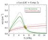 |
Fig. 4 Same as Fig. 3 for the sum of both velocity components toward α Leo. |
| In the text | |
|
Fig. 5 Lyman α profile in the spectrum of α Leo. The original data have been smoothed by 20 pixels to reduce the apparent noise. The red trace shows the expected profile from the two warm components with a total N(H I)tot = 1.9 × 1018 cm-2 (as favoured by our model). The blue trace shows the profile when an extra component with T = 200 000 K and N(H i) = 2.1 × 1015 cm-2 is added to the fit (see Sect. 7.5). In all models an absorption of D i is included,with a fixed D/H ratio of 1.6 × 10⁻⁵. |
| In the text | |
|
Fig. 6 Map of all secondary components, showing their velocity shift relative to the LIC component. This plot is the same as Fig. 12 of Gry & Jenkins (2014), but with one correction and a few additions including α Leo. Black asterisks signal the position of all targets. Blue/red squares mark secondary components with negative/positive shifts, and the size of the symbols scales with the amplitude of the shift. Dark blue symbols indicate the components having a uniform velocity shift of −7.2 ± 1.5km s-1 relative to the LIC (i.e. the Cetus Ripple); light blue symbols represent the other blue-shifted components. The blue circle at l = 2.3°, b = 31.4° shows the “Warm Breeze” heliospheric inflow direction. |
| In the text | |
Current usage metrics show cumulative count of Article Views (full-text article views including HTML views, PDF and ePub downloads, according to the available data) and Abstracts Views on Vision4Press platform.
Data correspond to usage on the plateform after 2015. The current usage metrics is available 48-96 hours after online publication and is updated daily on week days.
Initial download of the metrics may take a while.