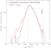
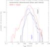
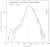
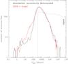
Fig. 4
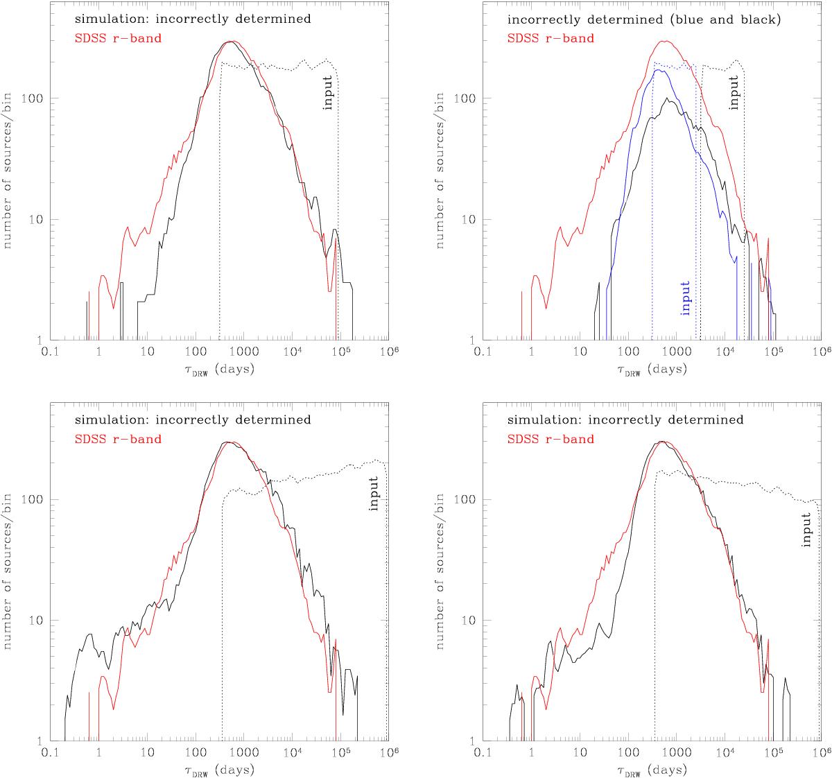
Simulations and modeling of 10 000 SDSS AGN light curves using DRW, where the input timescale is longer than 10% of the experiment span (from the “unconstrained” region in Fig. 2). The input distribution of τ is marked with dotted lines, while the output (measured) distribution of timescales is marked with the solid black/blue lines. The measured distribution of timescales for the real SDSS r-band AGN light curves is shown in red. It is obvious that DRW is unable to determine true decorrelation timescales if the input timescale is longer than 10% of the experiment span (if it belongs to the “unconstrained” region in Fig. 2). A flat input τ distribution is shown in the top left panel and is split into two flat distributions in the top right panel. In the bottom row, we used input distributions that are rising (left) and falling (right) with increasing τ. All the recovered distributions look akin to the SDSS one, and for the measured timescales longer than 100 days the KS test identifies the recovered and SDSS τ distributions as drawn from the same distribution. This simply means that the timescales obtained from SDSS (and in the future Gaia/LSST/Pan-STARRS) are unconstrained and should not be used to search for correlations with the physical parameters of AGNs, because the true values of τ and hence their distribution remains unknown.
Current usage metrics show cumulative count of Article Views (full-text article views including HTML views, PDF and ePub downloads, according to the available data) and Abstracts Views on Vision4Press platform.
Data correspond to usage on the plateform after 2015. The current usage metrics is available 48-96 hours after online publication and is updated daily on week days.
Initial download of the metrics may take a while.