| Issue |
A&A
Volume 597, January 2017
|
|
|---|---|---|
| Article Number | A76 | |
| Number of page(s) | 8 | |
| Section | Atomic, molecular, and nuclear data | |
| DOI | https://doi.org/10.1051/0004-6361/201628768 | |
| Published online | 04 January 2017 | |
MCDHF and RCI calculations of energy levels, lifetimes and transition rates for 3l3l′, 3l4l′, and 3s5l states in Ca IX – As XXII and Kr XXV⋆
1 Group for Materials Science and Applied Mathematics, Malmö University, 211 19 Malmö, Sweden
e-mail: This email address is being protected from spambots. You need JavaScript enabled to view it.
2 National Institute of Standards and Technology, Gaithersburg, MD 20899, USA
3 Oxford University, Mathematical Institute, Oxford OX2 6GG, UK
4 Cambridge University, Department of Applied Mathematics and Theoretical Physics, Centre for Mathematical Sciences, Cambridge CB3 0WA, UK
Received: 22 April 2016
Accepted: 18 July 2016
Abstract
Multiconfiguration Dirac-Hartree-Fock (MCDHF) calculations and relativistic configuration interaction (RCI) calculations were performed for states of the 3l3l′, 3l4l′ and 3s5l configurations in the Mg-like ions Ca IX – As XXII and Kr XXV. Valence and core-valence electron correlation effects are accounted for through large configuration state function expansions. Calculated excitation energies are in very good agreement with observations for the lowest levels. For higher lying levels observations are often missing and present energies aid line identification in spectra. Lifetimes and transition data are given for all ions. There is an excellent agreement for both lifetimes and transition data with recent multiconfiguration Hartree-Fock Breit Pauli calculations.
Key words: atomic data / methods: numerical / line: identification
Tables for energy levels, lifetimes, and transition data and full Tables 2, 4, and 6 are available at the CDS via anonymous ftp to cdsarc.u-strasbg.fr (130.79.128.5) or via http://cdsarc.u-strasbg.fr/viz-bin/qcat?J/A+A/597/A76
© ESO, 2017
1. Introduction
Mg-like ions are of considerable interest for diagnostic purposes in astrophysical plasmas and in fusion plasmas. The background and diagnostic details are given in Aggarwal et al. (2007) as well as in a series of comprehensive papers by Landi and Bhatia (Landi & Bhatia 2014; Bhatia & Landi 2011; Landi 2011).
During the past years a large number of calculations have been performed for Mg-like ions. In addition to the calculations above, see for example, Safronova et al. (2000), Froese Fischer et al. (2006), Massacrier & Artru (2012), Hu et al. (2014), Si et al. (2015), Santana & Träbert (2015). The most recent R-matrix calculations for the Mg-like ions include both collisional and radiative data (Fernandez-Menchero et al. 2014). Some of the calculations above provided data only for levels in the n = 3 complex but, as pointed out by Landi (2011), the real need is for data involving configurations with n ≥ 4.
Calculated excitation energies including low-frequency Breit and QED effects in cm-1 for Fe XV as a function of the increasing size of the CSF expansion.
In addition to energies and transition data involving configurations with n ≥ 4, there is also a need for transition energies that are accurate enough to aid line identifications. To meet these needs, systematic large scale relativistic multiconfiguration calculations were performed for states belonging to the 3l3l′, 3l4l′ and 3s5l′ configurations in the ions Ca IX – As XXII and Kr XXV. The present calculations provide a consistent and accurate data set for line identification and modeling purposes. The data set can also be used as a benchmark for other calculations.
2. Relativistic multiconfiguration calculations
The calculations were performed using the four-component fully relativistic multiconfiguration Dirac-Hartree-Fock (MCDHF) method relying on multireference single and double (MRSD) substitutions for generating wave function expansions. The method is described in detail in (Grant 2007) and in a recent review of multiconfiguration methods (Froese Fischer et al. 2016).
2.1. Multiconfiguration Dirac-Hartree-Fock
An atomic state is described by a wave function Ψ, that is a solution to the wave equation based on the Dirac-Coulomb Hamiltonian. In the MCDHF method, the wave function Ψ(γPJM) for a state labeled γPJM with γ being the orbital occupancy and angular coupling scheme, P the parity, and J and M the total angular quantum numbers, is expanded in configuration state functions (CSFs) 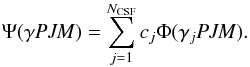 (1)The CSFs are antisymmetrized and symmetry-adapted many electron functions built from products of one-electron Dirac orbitals (Grant 2007; Froese Fischer et al. 2016).
The wave functions were determined in the extended optimal level (EOL) scheme and the radial parts of the Dirac orbitals and the expansion coefficients of the studied states were obtained iteratively in a layer by layer approach, as specified in Sect. 2.3, from a set of equations that results from applying the variational principle on a weighted energy functional of the studied states together with terms for preserving the orthonormality of the orbitals (Dyall et al. 1989). The transverse photon interaction in the low-frequency limit, or the Breit interaction (McKenzie et al. 1980), the mass polarization terms and the leading quantum electrodynamic (QED) effects (vacuum polarization and self-energy) were included in subsequent configuration interaction (RCI) calculations. In the RCI calculations the Dirac orbitals from the previous step were fixed, and only the expansion coefficients of the CSFs were determined by diagonalizing the Hamiltonian matrix. All calculations were performed with an updated parallel version of the GRASP2K code (Jönsson et al. 2013b).
2.2. Transition parameters
Transition parameters, such as transition rates or weighted oscillator strengths, between two states γ′P′J′ and γPJ, were expressed in terms of matrix elements of the transition operator (Grant 1974). In cases where the wave functions of the two states γ′P′J′ and γPJ were separately determined there are two orbital sets; one orbital set for γ′P′J′ and another orbital set for γPJ. Whereas the orbitals are orthonormal within each orbital set, orbitals for γ′P′J′ are not orthonormal to orbitals for γPJ. This complicates the evaluation of the matrix elements. To deal with this, the wave functions of the two states were transformed so that the orbital sets became biorthonormal (Olsen et al. 1995; Jönsson & Froese Fischer 1998), after which the calculation of the matrix elements was done using standard Racah algebra methods.
For electric multipole transitions, there are two forms of the transition operator: the length form and the velocity form (Grant 1974). Although the terms length and velocity form are applicable only to nonrelativistic calculations, in this paper we use them instead of the equivalent Babushkin and Coulomb gauges that are used in fully relativistic calculations such as ours. The length form is usually preferred, although the velocity form seems to be more stable for transitions including highly excited Rydberg states. The agreement between transition rates Al and Av computed in length and velocity forms can be used as an independent check on the accuracy of the wave functions that can be applied even when no values from observation are available (Froese Fischer 2009; Ekman et al. 2014). In this work the quantities 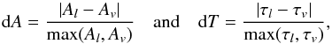 (2)were used as accuracy indicators for the transition rates and the lifetimes, respectively. The uncertainty indicators cannot be applied to a particular transition or level, but should instead be used in a statistical manner. The average root-mean-square (rms) value of the uncertainty indicator for a group of transitions that are similar in some sense can be used as an estimate for the uncertainty of transitions in this group. This is further discussed in Sect. 3.3.
Comparison of calculated and observed excitation energies in Ni XVII in cm-1.
Lifetimes in s. for Fe XV. τl and τv are lifetimes in length and velocity form, respectively.
2.3. Calculations
Calculations were performed for states belonging to the 3s2, 3p2, 3s3d, 3d2, 3s4s, 3s4d, 3p4p, 3p4f, 3d4s, 3d4d, 3s5s, 3s5d, 3s5g even configurations and the 3s3p, 3p3d, 3s4p, 3p4s, 3s4f, 3p4d, 3d4p, 3d4f, 3s5p, 3s5f odd configuration. These configurations define the multireference (MR) for the even and odd parities, respectively. As a starting point an MCDHF calculation for all even and odd reference states was done in the EOL scheme. The initial calculation was followed by separate calculations in the EOL scheme for the even and odd parity states. The calculations for the even states were based on CSF expansions obtained by allowing single (S) and double (D) substitutions of orbitals in the even MR configurations to an increasing active set of orbitals. In a similar way the calculations for the odd states were based on CSF expansions obtained by allowing single (S) and double (D) substitutions of orbitals in the odd MR configurations to an increasing active set of orbitals. To prevent the CSF expansions to grow unmanageably large, at most single substitutions were allowed from the 2s and 2p subshells. The 1s shell was always closed. The CSF expansions account for valence and core-valence electron correlation. Remaining correlation effects, mainly core-core correlation, are comparatively unimportant for both the excitation energies and the transition probabilities for such highly ionized systems. The active sets of orbitals for the even and odd parity states were extended by layers to include orbitals with quantum numbers up to n = 8 and l = 6. Each layer of active orbitals were optimized separately in the EOL scheme, with the previous layers kept frozen. The MCDHF calculations were followed by RCI calculations, including mass-polarization, the Breit-interaction and leading QED effects. The number of CSFs in the final even and odd state expansions were approximately 640 000 and 630 000, respectively, distributed over the different J symmetries.
2.4. Labeling of states
In order to identify the computed states and match them against observations, the wave function expansions over jj-coupled CSFs were transformed to LSJ coupling (Gaigalas et al. 2003). In all tables of this paper the quantum states are labeled with the leading term of the LSJ-percentage composition. The labels obtained with this approach are, however, not unique and this is further discussed in the next section.
3. Results and discussion
3.1. Energies
In Table 1 we present the computed excitation energies for the 35 lowest levels in Fe XV belonging to the 3l3l′ configurations as functions of the increasing active sets of orbitals labeled with the highest principal quantum number n of the orbitals in the set. For comparison, observed energies from the NIST Atomic Spectra Database (ver. 5.3; Kramida et al. 2015) are given as well. The relative differences between theory and observation are 0.122%, 0.49%, 0.050% and 0.041% for calculations based on the expansion from the MR and the expansions from SD excitations to orbital sets with the highest principal quantum numbers n = 6,7,8. Looking more carefully at Table 1 it is seen that the triplet states show better convergence properties than the singlet states. For the singlet states the relative differences between theory and observation are 0.233%, 0.789%, 0.106% and 0.073% and the singlet states are not fully converged with respect to the orbital set. Adding a few orbital layers would improve the excitation energies, but would add to the total computation time. Differences in convergence rates are further analyzed and discussed in Jönsson et al. (2016). In Table 2 the computed excitation energies for Ni XVII (the full table for Ca IX – As XXII and Kr XXV is available at the CDS) based on the largest orbital set n = 8 are displayed together with observed energies from the NIST Atomic Spectra Database (ver. 5.3; Kramida et al. 2015). The differences between the computed and observed energies are also given. For Kr XXV, excitation energies from accurate many-body perturbation calculations by Si et al. (2015) can be used for further comparisons.
The agreement between the computed excitation energies and the observed energies is generally very good, although the calculations give somewhat too high excitations energies for the states belonging to the 3l4l′ and 3s5l configurations. For these states typical differences are between 1000 cm-1 and 2000 cm-1, which translates to relative differences of theory and observation between 0.05% and 0.1%. The difference between calculations and observations can be explained by the fact that the current calculations extend to many configurations and that the calculations are not fully converged with respect to the orbital basis. The difference is also due to the fact that core-core electron correlation were neglected, the effect of which is to lower the energies of the higher lying states. There are many states for which theory and observations do not agree at all. An example is 3s4d 1D2, where the difference is −4488 cm-1 in Sc X and 6498 cm-1 in Ti XI. These disagreements may be due to difficulties in identification or labeling of levels derived from observed data. The present data are useful in validating the identification of levels.
As for most calculations involving states of many configurations there are labeling problems (Jönsson et al. 2013a). States are often labeled by the leading term of the wave function LSJ-percentage composition. For closely lying interacting states with the same J, the leading term can be the same. To resolve this the label can be based on more terms of the composition. A simpler solution is to add an extra index to the leading term of the composition. We choose the latter solution. For example, the two J = 3 states in Fe XV at 2 316 401 cm-1 and 2 333 084 cm-1 both have the leading term 3p4d 3D3. These two states were labeled 3p4d 3D3 a and 3p4d 3D3 b, respectively. It is important to realize that the wave function LSJ-percentage composition depends on the details of the calculation, and thus two calculations can have slight differences in compositions leading to differences in labels.
3.2. Lifetimes
Lifetimes of the excited states were calculated from E1 and M1 transition rates. The contributions to the lifetimes from E2 and higher multipoles are negligible. In Table 3 the present lifetimes for the 84 lowest states in Fe XV in length and velocity form are compared with lifetimes from the multiconfiguration Hartree-Fock Breit-Pauli (MCHF-BP) calculations by Froese Fischer et al. (2006) and with the CIV3 calculations by Aggarwal et al. (2007). Included in the table are also lifetimes from beam-foil measurements by Hutton et al. (1988).
The average relative difference between the lifetimes in the length and velocity forms from the present calculation is less than 0.52%, which is highly satisfactory. This difference can be seen as an internal validation of the accuracy. The differences between the present lifetimes in the length form and the lifetimes by Froese Fischer et al. (2006) and Aggarwal et al. (2007) are 1.37% and 4.45%, respectively. Comparing theoretical and experimental lifetimes we see that they do not agree very well. This may be due to large uncertainties in the beam-foil measurements as discussed in Zou et al. (1999). In Table 4 the computed lifetimes in length form and the uncertainty estimators dT are displayed for Fe XV (the full table for Ca IX – As XXII and Kr XXV is available at the CDS) based on the largest orbital set n = 8.
3.3. Oscillator strengths and transition rates
In Table 5 the present oscillator strengths in the length form for selected transitions in Fe XV are compared with values from the MCHF-BP calculations by Froese Fischer et al. (2006) and with values from the CIV3 and MCDHF calculations by Aggarwal et al. (2007). Values from the present calculations and the MCHF-BP calculations agree to within 1.53%. The agreement with the CIV3 and MCDHF calculations by Aggarwal et al. (2007) is 8.42% and 6.50%, respectively. The results of the comparisons are explained by the fact that the RCI and MCHF-BP calculations include more electron correlation effects than do the CIV3 and MCDHF calculations. Due to the neglected electron correlation two the latter calculations are believed to be somewhat less accurate.
Lifetimes in s for Fe XV.
Oscillator strengths f for selected transitions in Fe XV.
Transition data for Fe XV.
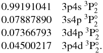
In Table 6 the transition energies, wavelengths, transition rates A, and weighted oscillator strengths gf are given for Fe XV (the full table for Ca IX – As XXII and Kr XXV is available at the CDS). All E1 and M1 transitions with rates A larger than 104 s-1 are displayed. Transition data are also given for transitions with rates A greater than a fraction 10-4 of the sum of the A-values for transitions from the upper level. For the E1 transitions also the uncertainty indicator dA is given. For most of the stronger E1 transitions dA is below 1%. For the weaker transitions the situation is somewhat different. While many of the weaker transitions have dA in the range from a few percent up to 10% there are also many transitions for which dA is considerably larger. These transitions are often so called two-electron one-photon transitions for which the configurations involved in the transitions differ by two electrons. For two-electron one-photon transitions the rate between two states is determined, not from the major CSFs that define the label, but from other CSFs of the wave function expansion, often CSFs that are part of the MR set. We take the  transition in Ca IX at 499.614 Å as an example. The rate is A = 1.716 × 10⁶ s-1 and dA = 0.166. In LSJ coupling the major contributors to the states are
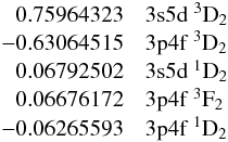 and
and
 Due to the selection rules of the transition operator, contributions to A are zero from the two dominating CSFs of the even state to the dominating CSF of the odd state. The transition rate A is instead determined by contributions from different combinations of the remaining CSFs. The lack of contributions from the dominating CSFs together with many smaller and canceling contributions from the remaining CSFs often make the two-electron one-photon transitions weak and with large values of dA. Although important and challenging from a theoretical point of view, these weak transitions have little practical importance in modeling applications.
3.4. Summary and conclusions
MCDHF and subsequent RCI calculations were performed for states of the 3l3l′, 3l4l′ and 3s5l configurations in the Mg-like ions Ca IX – As XXII and Kr XXV and excitation energies, lifetimes, and transition data are presented for all ions. Excitation energies from the RCI calculations are in very good agreement with available observations for the lower states. For the higher states the calculated excitations energies are 1000 cm-1–2000 cm-1 larger than energies from observations. There are also anomalous differences, either positive or negative, between calculations and observations due to misindentifications. One example is the 3p4f configuration in Cu XVIII. Here the difference between calculations and observations are 22 083 cm-1 and 1432 cm-1 for 3p4f 3D3 and 3p4f 3D2, respectively. The former difference indicates a misidentification of observed data.
Lifetimes were internally validated by comparing values in length and velocity form. Lifetimes in the two forms differ in average at the 0.5% level. Systematic comparisons with the MCHF-BP calculations by Froese Fischer et al. (2006) showed that lifetimes from these two calculations differ on average only by 1.5%. Also for the oscillator strengths the present calculations showed good consistency with the MCHF-BP with an average relative difference of 1.5% for selected transitions in Fe XV. Uncertainties of the transition rates are estimated by dA, as suggested by Ekman et al. (2014). For most of the stronger transitions, dA is below 1%. The transition rates for many of the weak two-electron one-photon transitions are highly uncertain, as indicated by large values of dA.
Acknowledgments
S.G. and P.J. acknowledge support from the Swedish Research Council under Grant 2015-04842.
References
- Aggarwal, K. M., Tayal, V., Gupta, G. P., & Keenan, F. P. 2007, At. Data Nucl. Data Tables, 93, 615 [NASA ADS] [CrossRef] [Google Scholar]
- Bhatia, A. K., & Landi, E. 2011, At. Data Nucl. Data Tables, 97, 189 [NASA ADS] [CrossRef] [Google Scholar]
- Dyall, K. G., Grant, I. P., Johnson, C. T., Parpia, F. A., & Plummer, E. P. 1989, Comput. Phys. Commun., 55, 425 [NASA ADS] [CrossRef] [Google Scholar]
- Ekman, J., Godefroid, M. R., & Hartman, H. 2014, Atoms, 2, 215 [NASA ADS] [CrossRef] [Google Scholar]
- Hu, F., Mei, M., Han, C., et al. 2014, J. Quant. Spectrosc. Radiat. Trans., 149, 158 [NASA ADS] [CrossRef] [Google Scholar]
- Fernandez-Menchero, L., Del Zanna, G., & Badnell, N. R. 2014, A&A, 572, A115 [NASA ADS] [CrossRef] [EDP Sciences] [Google Scholar]
- Froese Fischer, C. 2009, Phys. Scr. T, 134, 014019 [Google Scholar]
- Froese Fischer, C., Tachiev, G., & Irimia, A. 2006, At. Data Nucl. Data Tables, 92, 607 [NASA ADS] [CrossRef] [Google Scholar]
- Froese Fischer, C., Godefroid, M., Brage, T., Jönsson, P., & Gaigalas, G. 2016, J. Phys. B: At. Mol. Opt. Phys., submitted [Google Scholar]
- Gaigalas, G., Žalandauskas, T., & Rudzikas, Z. 2003, At. Data Nucl. Data Tables, 84, 99 [NASA ADS] [CrossRef] [Google Scholar]
- Grant, I. P. 1974, J. Phys. B, 7, 1458 [Google Scholar]
- Grant, I. P. 2007, Relativistic Quantum Theory of Atoms and Molecules (New York: Springer) [Google Scholar]
- Hutton, R., Engström, L., & Träbert, E. 1988, Nucl. Instrum. Meth. Phys. Res. B, 31, 294 [NASA ADS] [CrossRef] [Google Scholar]
- Jönsson, P., & Froese Fischer, C. 1998, Phys. Rev. A, 57, 4967 [NASA ADS] [CrossRef] [Google Scholar]
- Jönsson, P., Ekman, J., Gustafsson, S., et al. 2013a, A&A, 559, A100 [NASA ADS] [CrossRef] [EDP Sciences] [Google Scholar]
- Jönsson, P., Gaigalas, G., Bieroń, J., Froese Fischer, C., & Grant, I. P. 2013b, Comput. Phys. Commun., 184, 2197 [NASA ADS] [CrossRef] [Google Scholar]
- Jönsson, P., Radžiūtė, L., Gaigalas, G., et al. 2016, A&A, 585, A26 [NASA ADS] [CrossRef] [EDP Sciences] [Google Scholar]
- Kramida, A., Ralchenko, Yu., Reader, J., & NIST ASD Team 2015, NIST Atomic Spectra Database (ver. 5.3), available: http://physics.nist.gov/asd [2016, April 5] (Gaithersburg, MD: National Institute of Standards and Technology) [Google Scholar]
- Landi, E. 2011, At. Data Nucl. Data Tables, 97, 587 [NASA ADS] [CrossRef] [Google Scholar]
- Landi, E., & Bhatia, A. K. 2014, At. Data Nucl. Data Tables, 100, 1519 [NASA ADS] [CrossRef] [Google Scholar]
- Massacrier, G., & Artru, M.-C. 2012, A&A, 538, A52 [NASA ADS] [CrossRef] [EDP Sciences] [Google Scholar]
- McKenzie, B. J., Grant, I. P., & Norrington, P. H. 1980, Comput. Phys. Commun., 21, 233 [NASA ADS] [CrossRef] [Google Scholar]
- Olsen, J., Godefroid, M., Jönsson, P., Malmqvist, P. Å., & Froese Fischer, C. 1995, Phys. Rev. E, 52, 4499 [NASA ADS] [CrossRef] [Google Scholar]
- Safronova, U. I., Johnson, W. R., & Berry, H. G. 2000, Phys. Rev. A, 61, 052503 [NASA ADS] [CrossRef] [Google Scholar]
- Santana, J. A., & Träbert, E. 2015, Phys. Rev. A, 91, 022503 [NASA ADS] [CrossRef] [Google Scholar]
- Si, R., Guo, X. L., Yan, J., et al. 2015, J. Phys. B: At. Mol. Opt. Phys., 48, 175004 [NASA ADS] [CrossRef] [Google Scholar]
- Zou, Y., Hutton, R., Huldt, S., et al. 1999, Phys. Scr.. T, 80, 460 [Google Scholar]
All Tables
Calculated excitation energies including low-frequency Breit and QED effects in cm-1 for Fe XV as a function of the increasing size of the CSF expansion.
Lifetimes in s. for Fe XV. τl and τv are lifetimes in length and velocity form, respectively.
Current usage metrics show cumulative count of Article Views (full-text article views including HTML views, PDF and ePub downloads, according to the available data) and Abstracts Views on Vision4Press platform.
Data correspond to usage on the plateform after 2015. The current usage metrics is available 48-96 hours after online publication and is updated daily on week days.
Initial download of the metrics may take a while.