| Issue |
A&A
Volume 597, January 2017
|
|
|---|---|---|
| Article Number | A83 | |
| Number of page(s) | 12 | |
| Section | Celestial mechanics and astrometry | |
| DOI | https://doi.org/10.1051/0004-6361/201628717 | |
| Published online | 06 January 2017 | |
Evaluation of a possible upgrade of the IAU 2006 precession
1 School of Astronomy and Space Science, Key Laboratory of Modern Astronomy and Astrophysics (Ministry of Education), Nanjing University, 163 XianLin Avenue, 210023 Nanjing, PR China
e-mail: This email address is being protected from spambots. You need JavaScript enabled to view it.
2 SYRTE, Observatoire de Paris, PSL Research University, CNRS, Sorbonne Universités, UPMC Univ. Paris 06, LNE, 61 avenue de l’Observatoire, 75014 Paris, France
e-mail: This email address is being protected from spambots. You need JavaScript enabled to view it.
Received: 14 April 2016
Accepted: 8 September 2016
Abstract
Context. The International Astronomical Union (IAU) adopted a new precession model at its 2006 General Assembly. After more than ten years since the publication of the so-called IAU 2006 precession, we have noticed progress in solar system ephemerides and geophysical observations, which can be used to refine the precession model. Another progress is the increase by 30% since 2003, of the length of the very long baseline interferometry (VLBI) observations to be compared with the theoretical model.
Aims. The aim of this paper is to investigate the possibility of upgrading the IAU 2006 precession model based on new solutions of the Earth-Moon barycenter (EMB) motion, new theoretical contributions to the precession rates, and the revised J2 long-term variation obtained from the satellite laser ranging (SLR).
Methods. The new precession expressions for the ecliptic are derived by fitting the new analytical planetary theory VSOP2013 to the numerical ephemerides DE422 or INPOP10a. The solution for the precession of the equator was obtained by integrating the dynamical precession equations with the use of an updated Earth model including the J2 quadratic long-term variation. The new precession expressions (denoted LC solution in this paper) are compared with the IAU 2006 model by using the most accurate VLBI observations up to 2015.
Results. For the precession of the ecliptic, the changes in the new solutions with respect to the IAU 2006 are about several tens of microarcseconds in the linear terms of PA and QA. The upgraded precession of the equator is such that the quadratic and cubic terms in the quantity ψA differ significantly from IAU 2006 due to the revised J2 model. The statistics of the VLBI celestial pole offsets (1979–2015) and least squares fits with different empirical models, show that the LC precession is slightly more consistent with the VLBI observations, but the improvement relative to the IAU 2006 model is not definitely convincing at present.
Conclusions. The upgraded LC precession obtained with the latest theoretical and observational improvements has shown some advantages with respect to the IAU 2006 model. However, due to negligible changes in the precession of the ecliptic and large uncertainties in the J2 variation, we recommend that the standard IAU 2006 model be retained for practical use and continuity reason. The next precession-nutation model should be constructed with a uniform dynamical approach in the framework of ICRF3 and Gaia reference frame and without the use of a conventional ecliptic.
Key words: astrometry / celestial mechanics / reference systems / ephemerides
© ESO, 2017
1. Introduction
The current standard precession-nutation model recommended by the International Astronomical Union (IAU) and the International Earth Rotation and Reference System Service (IERS) is composed of the IAU 2006 precession (Capitaine et al. 2003a; Hilton et al. 2006, also known as P03 model) and the IAU 2000A nutation series (Mathews et al. 2002) with IAU 2006 adjustments. In order to be most compatible with the IAU 2000 nutation and to provide polynomial developments for a number of quantities for use in both equinox based and CIO (Celestial intermediate origin) based celestial-to-terrestrial reference system transformation paradigms, the IAU 2006 precession computations followed the traditional way in which a time-dependent “ecliptic” (i.e., a kind of representation of the mean orbital motion of the Earth-Moon barycenter (EMB) in the Geocentric Celestial Reference System (GCRS)) was used as an intermediate plane for expressing the contributions to the precession rates resulting from the external torques induced by the Sun, the Moon, and the planets. Capitaine et al. (2004) compared the P03 precession with other post-2003 developments, such as F03 (Fukushima 2003), HF04 (Harada & Fukushima 2004), B03 (Bretagnon et al. 2003), and W94 (Williams 1994) models, concluding that the P03 precession of the ecliptic and equator were the most accurate among various solutions. From observational and practical points of view, the P03 precession model is consistent with the very long baseline interferometry (VLBI) observations, therefore is quite efficient for predicting the secular motion of the Celestial Intermediate Pole (CIP) in the GCRS. These are the reasons why the IAU adopted the P03 solution as the standard IAU 2006 model in the Prague General Assembly.
The IAU 2006 precession of the ecliptic (Capitaine et al. 2003a) was derived by fitting the analytical ephemerides VSOP87 (Bretagnon & Francou 1988) to the long-term numerical ephemerides DE406 (Standish 1998) over the time span J1000.0 to J3000.0. The best rotations from DE406 equatorial coordinate system to the ecliptic system were found, then the corrections restricted by observational data (namely DE406) were applied to VSOP87 polynomial expressions for the osculating elements p and q, which represent the secular motion of the moving ecliptic pole in the fixed ecliptic coordinate system of J2000. The final solution was used to replace the IAU 1976 expressions for the precession of the ecliptic (Lieske et al. 1977).
Regarding the precession of the equator, the previous version, the IAU 2000 model (Mathews et al. 2002), consists only of corrections to the precession rates in longitude and obliquity of the IAU 1976 precession. The effect of the changes on the higher-order terms in the precession theory were ignored; thus the IAU 2000 precession was not consistent with the dynamical theory of the Earth’s rotation. The IAU 2006 precession of the equator (Capitaine et al. 2003a), in contrast, is dynamically consistent: the basic precession quantities ψA and ωA were derived by solving the dynamical differential equations using improved ecliptic precession, integration constants provided by IAU 2000 precession with careful consideration of perturbing effects, and the best non-rigid Earth model available at that time. One notable progress of the IAU 2006 precession of the equator is the inclusion of a negative J2 rate (J2 is known as the Earth’s form factor or the second-degree zonal harmonic of the Earth’s gravitational field) that is generally attributed to the postglacial rebound of the Earth’s mantle. The value for the J2 rate adopted in the IAU 2006 model is  (1)corresponding to
  (2)The contribution of this linear change in J2 to the precession rate in longitude, rψ, is of −14 mas t, which yields about −7 mas t2 in the polynomial expression for ψA. This is the main reason for the quadratic term difference between the IAU 2006 and IAU 2000 equator precession in longitude. However, the relative uncertainty of the J2 rate is about 20% (Williams 1994), which is the main limiting factor of the accuracy of the precession in longitude. Thereafter Capitaine et al. (2005, denoted P04 paper) tried to improve the P03 precession of the equator using a refined model for the contribution of non-rigid Earth and revised integration constants from VLBI data. The conclusion was to retain the P03 solution as the replacement for the IAU 2000 model due to the fact that there was no convincing evidence that the P04 would deliver better accuracy than the P03 precession model.
Since the publication of the IAU 2006 precession in 2003, more accurate analytical and numerical ephemerides for the solar system planets, which provide improved EMB motion, have been made available for recalculating the precession of the ecliptic. Moreover, updated theoretical contributions to the precession rates and observations for the Earth’s gravitational field enable us to look into the possibility of improving the precession of the equator. This paper reports our effort to develop refined precession solutions based on these scientific advancements.
2. Improving the precession of the ecliptic
The ecliptic pole is defined by the mean orbital angular momentum of the Earth-Moon barycenter (EMB) about the Sun (rather than the solar system barycenter, SSB) in the Barycentric Celestial Reference System (BCRS). The precession of the ecliptic is defined as the secular part of the ecliptic pole motion in the initial reference system and is represented by the parameters PA and QA:  (3)where πA is the inclination of the moving ecliptic to the fixed ecliptic, and ΠA is the longitude of the node of the moving ecliptic upon the fixed ecliptic of J2000.0. The analytical planetary theories Variations Séculaires des Orbites Planétaires (VSOP, Bretagnon & Francou 1988) introduced the equinoctial elements p and q for the Earth-Moon barycenter:
  (4)The rigorous relations between PA, QA, and p, q are such that:
  (5)
(5)
2.1. The analytical planetary theory VSOP2013 and the numerical ephemerides DE422 INPOP10a
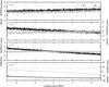 |
Fig. 1 Difference of PA and QA between various ephemerides used in this paper over 20 centuries (1000−3000). A different scale is used in the bottom plot (d). |
Since the IAU 2006 precession of the ecliptic had been derived using VSOP87 (Bretagnon & Francou 1988) and DE406 (Standish 1998), progress in the solutions for the EMB motion have been made. The new analytical planetary theory VSOP2013, together with the Theory of the Outer Planets TOP2013 were developed by Simon et al. (2013). The VSOP2013 is fitted to the INPOP10a (Intégrateur Numérique Planétaire de l’Observatoire de Paris) numerical planetary ephemeris (Fienga et al. 2011) and the accuracy between 1890 and 2000 is improved by a factor two to 24 depending on the planets, as compared to its previous version VSOP2000. The long-term data (from −4000 to 8000, used in this study) is more accurate by a factor of five with respect to VSOP2000. Since the VSOP2000 solution was ten to 100 times more precise than the VSOP87 as used in the IAU 2006 model (Simon et al. 2013), the improvement of VSOP2013 with respect to VSOP87 is quite remarkable. The VSOP2013 has provided numerical Chebyshev Ephemerides from −4500 to 4500 with a similar structure to DE ephemerides (Jet Propulsion Laboratory Development Ephemeris). It also provides users with the elliptic elements, including p and q, for the eight planets in the form of mixed series which contain secular, Fourier, and Poisson terms. The secular parts (polynomials up to the eighth degree in t) of p and q for EMB motion representing the precession of the ecliptic will be studied in the following.
The JPL DE422 numerical ephemerides (Folkner et al. 2008), covering the time interval between JD 0625648.5 (December 7, 3001 BC) and JD 2816816.5 (January 30, 3000 AD), was created in 2009. It is referred to the International Celestial Reference Frame (ICRF) and includes nutations and liberations. DE422 has made use of new observations including ranging data from Mars spacecrafts, the effects of nutation and libration of the Moon, Venus Express (VEX) ranging data for the improvement of Venus orbit, and Cassini data for better constraints on Jupiter and Saturn orbits. All these data improved the estimation of EMB orbit, the strongest constraints being given by the ranging data from Mars spacecraft.
The numerical ephemerides INPOP10a, also in the framework of the ICRF, was developed by Fienga et al. (2011) and was released in 2010. As compared to the previous INPOP versions, several improvements have been introduced in the fitting process, the data sets used in the fit, and the selection of fitted parameters. More than 136 000 planetary observations including the latest Messenger, Mars Express, Venus Express, and Cassini data, and lunar laser ranging (LLR) normal points have been applied for the construction of INPOP. The main characteristics are the fit of the product, GM⊙, of the solar mass with the gravitational constant instead of the astronomical unit, and the determinations of the post-Newtonian (PPN) parameters as well as adjustments of the solar oblateness and of asteroid masses. The new IAU resolution about the astronomical unit (AU, Capitaine et al. 2011) was implemented for the first time in INPOP10a, together with the best estimations of the mass of planets provided by the IAU 2009 solution (Luzum et al. 2011). Statistics of planetary post residuals after fit show that the accuracy of the INPOP10a has been largely improved in comparison to the previous version INPOP08 (Fienga et al. 2010).
2.2. Revision of the ecliptic precession based on new developments
In this subsection we show the possibility of improving the ecliptic precession by fitting VSOP2013 theory to DE422/INPOP10a: the later ephemerides are introduced as additional constrains. The purpose of using both modern numerical ephemerides prolongated over the same time span (1000−3000) is to investigate the effect of different ephemerides on the estimation of the ecliptic precession.
For VSOP2013, PA and QA are obtained directly using elliptic elements p, q with Eq. (5). For DE422 or INPOP10a, we first interrogate the ephemerides to obtain the EMB heliocentric position r and velocity ṙ in the International Celestial Reference System (ICRS, i.e., the equatorial coordinate system) and calculate the angular momentum:  (6)In the next step, the components of the angular momentum h are transformed from the ICRS to the J2000 ecliptic frame using the following equation:
  (7)where the geometrical definition of the angles ψ0, ϵ0, and φ0 are given in Fig. 1 of Capitaine et al. (2003a). Initially, the values are provided by VSOP2013 (Simon et al. 2013) as
  (8)At last, the parameters PA and QA for DE422 and INPOP10a can be derived from the vector
  in the ecliptic coordinate system:
  (9)considering that PA and QA are the x and −y components of the moving ecliptic pole vector in the fixed ecliptic at J2000. | hecl | is the norm of the vector hecl.
Figure 1 (panels a–c) shows the difference between DE422, INPOP10a, and VSOP2013 for the EMB motion represented by PA and QA in the dynamical ecliptic frame over 20 centuries, while the bottom panel (d) is the same plot for the difference [DE406 − VSOP87] which were studied in the IAU 2006 model (see similar Figs. 2 and 4 of Capitaine et al. 2003a). The thickness of the curves is due to the short periodic terms; the slope and curvature are attributed to the misalignment of the secular part; the overall offset of the curves is due the imperfection of the transformation angles between the ecliptic and equatorial coordinate system. For the last panel, original transformation angles in the P03 paper (ψ0 = 0,  , and φ0 = 0) are applied, which cause large offsets between PA and QA. Panel d in Fig. 1 clearly displays that the secular discrepancy [DE422 − VSOP2013] or [INPOP10a − VSOP2013] is significantly less than [DE406 − VSOP87] because the VSOP87 analytical theory was fitted to the DE200 ephemerides (constructed in 1981), and thus was not up-to-date relative to DE406 (constructed in 1995) at the time of developing the IAU 2006 precession.
Equator to Ecliptic coordinate system transformation angles for DE422 and INPOP10a.
The situation has now changed: the more recent ephemerides VSOP2013, INPOP10a, and DE422 have the same level of accuracy, therefore, in principle, either VSOP2013, INPOP10a, or DE422 can be used to construct the precession of the ecliptic independently. However, using only numerical ephemerides could bring a risk of contamination by long periodic terms. Capitaine et al. (2004) compared various precession models of the ecliptic and found that the F03 (Fukushima 2003) and HF04 (Harada & Fukushima 2004) models fitted to DE405 over hundreds of years seriously deviate from observations because they are largely affected by residual contributions of long period terms that have been incorrectly dealt with. On the other hand, the IAU 2006 (Capitaine et al. 2003a) model avoided this problem without any bias through a fit of VSOP87 to DE406 in the interval 1000−3000. Here, we follow a similar approach by a fit of VSOP2013 to DE422/INPOP10a in order to obtain the final secular part of the EMB motion.
Corrections Δp and Δq to VSOP2013 secular terms.
Precession quantities of the ecliptic derived from VSOP2013 and DE422/INPOP10a ephemerides and comparison with the IAU 2006 model.
The 250-day sampling series of (t, Δp, Δq) in the sense of [DE422/INPOP10a − VSOP2013] between J1000 and J3000 are fitted to the fifth order polynomials. The resulting coefficients of constant terms p0 and q0 are used to improve the rotation angles, while the coefficients of t1−t5 terms are added to corresponding secular terms given by VSOP2013. Only two iterations are required to reach the converged results. The final rotation angles from equatorial to ecliptic coordinate systems for DE422 and INPOP10a are presented in Table 1. The total corrections, along with their uncertainties to be added to the secular variations of p and q (except for the constant terms), are given in Table 2, where the numerical coefficients are in microarcseconds (μas), and t is measured in Julian centuries elapsed from J2000.0. PA and QA are transformed from p and q discrete points using Eq. (5) and then fitted to the fifth order polynomial to derive the coefficients from t1 to t5. Table 3 gives the updated ecliptic precession quantities PA and QA corresponding to the values in Table 2. In this way, the real uncertainties of the PA and QA polynomial coefficients are not easy to derive: they should depend on the errors in the used ephemerides. Since PA/QA and p/q are equivalent, the error of t1 coefficients of PA and QA should not exceed several microarcseconds per year, while the errors in higher order terms are too small to be considered. The above Tables 2 and 3 illustrate the following points:
-
in Table 2, the difference between linear termsof p and q between DE422, INPOP10a, and VSOP2013 are at the order of several tens of microarcseconds, while higher order terms are negligible;
-
from both tables, we found that the VSOP2013 EMB secular motion is closer to DE422 than to INPOP10a, although VSOP2013 was nominally fitted to INPOP10a;
-
the discrepancy of the solution for the precession of the ecliptic PA and QA in the present work and IAU 2006 model is several tens of microarcseconds for linear term and about 10 μas for square term.
-
in fact, the difference in precession of the ecliptic between our new solution and the IAU model is about two orders of magnitudes lower than [IAU 2006 − other post-2003 solution] which shows good agreement between current results and the IAU 2006 model. Here “post-2003 solutions” refer to F03 (Fukushima 2003), HF04 (Harada & Fukushima 2004), B03 (Bretagnon et al. 2003), and W94 (Williams 1994) solutions.
According to the comparative study in Capitaine (2004), a difference in the t term of PA and/or QA is fully reflected in the coefficients for ϵA and/or χA expressions, both referring directly to the ecliptic. On the other hand, the largest effect in the basic quantities for the precession of the equator, ψA and ωA expressions, is of the order of 0.1 mas in the t2 term for a difference of a few mas in the t term of PA and/or QA. This means that the changes given by Table 3 would give effects of the order of tens of μas in the t term of ϵA and/or χA, and of only about of 1 μas in the t2 terms of ψA and ωA. This order of effect is not crucial for deriving the precession of the equator as compared to the improved theoretical contributions, especially that due to the updated J2 variation (see Sect. 3.1). The above conclusions have been verified by testing both ecliptic precession for DE422 and INPOP10a: very similar expressions for the precession of the equator are obtained. Given that small difference, we will provide in the following sections, only the solution for the precession of the equator corresponding the DE422-derived ecliptic precession (cf. lines 1 and 3 of Table 3).
3. Improving the precession of the equator based on recent progress
The solutions for the precession of the equator are derived by solving the differential equations given in Williams (1994) or Capitaine et al. (2003a): 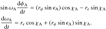 (10)The classical precession quantities ψA and ωA are chosen as primary parameters because they can be regarded as the angular coordinates of the CIP (or moving equator) with respect to the fixed J2000 ecliptic and the specified precession-rate adjustments can be applied directly and unambiguously.
The above equations transform the precession rates of the mean celestial pole in longitude and obliquity (rψsinϵA and rϵ) from the moving ecliptic system to the fixed ecliptic system through the angle χA, which is called planetary precession measured along the moving equator between the intersections of the moving ecliptic and the fixed ecliptic1. The other two equations for precession quantities pA (general precession) and ϵA (obliquity of date) are solved simultaneously with the geometrical relation  (11)The resolution of the above equations for computing the IAU 2006 precession was based on the use of a semi-analytical method (with GREGOIRE software, see description in the appendix of Capitaine et al. 2003b). In the present work, we follow a universal numerical approach that has been verified to give the same results for the IAU 2006 case. First, the classical 7(8)-degree Runge-Kutta-Fehlberg (RKF) method2 was employed to derive the discrete points (250-day step over 2000 yr centered on J2000.0) for basic quantities ψA, ωA and secondary quantities ϵA, χA, and pA, then the fifth order polynomial expressions for these quantities are obtained by an unweighted least squares fit.
In order that the refined solution for the precession of the equator be “dynamically consistent” and compliant with the IAU 2000 nutation, we proceed with our computation in the same way as IAU 2006. This means solving the above differential Eq. (10) with the use of (1) the best available expressions for PA and QA for the precession of the ecliptic; (2) theoretical corrections to precession rates; (3) the best available integration constants r0 and u0 at J2000.0. The first subject relating to the ecliptic motion has been studied in Sect. 2, so in Sects. 3.1 and 3.2 we investigate the possible improvements in the latter two aspects, respectively, and give the final expression in Sect. 3.3.
3.1. Upgraded contributions to the precession rates
The theoretical expressions for the precession rates with respect to the moving ecliptic can be written as: 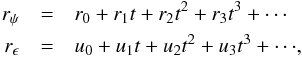 (12)where the complete list for the theoretical contributions are provided in Table 3 of Capitaine et al. (2003a). The new progress in precession rates since 2003, within our knowledge, includes the following items:
-
i.
Post-Newtonian treatment of the Earth’s rotation in theframework of General Relativity (Gerlach & Klioner 2013). Thegeodesic precession-induced torque is taken into account toobtain the Euler angles of rigid Earth (φ, ψ, ω, the later two correspond to precession quantities in longitude and obliquity, while φ is related to the rotation rate around the pole) in the kinematically non-rotating GCRS. The discrepancies between the SMART solution (Bretagnon et al. 1997) and corrected solutions for the Euler angles are shown to be Poisson-like and the amplitudes after one century are about 200 μas in ψ and 100 μas in ω (see Fig. 2 of quoted paper). The slope of the discrepancy is not clearly visible from the plots and not provided by the authors, therefore this effect was not considered in our computation.
-
ii.
Determination of the J2 long-term variation based on satellite laser ranging (Cheng et al. 2013). This will be discussed in detail in the following.
-
iii.
The contribution of tidal Poisson terms on non-rigid Earth rotation (Folgueira et al. 2007). The Poisson terms in the tidal potential generated by solar system bodies contributes 88μas cy-1 to the precession rate in obliquity. It is useful to mention that the largest contribution to nutation in longitude, although not used directly in the integration, is 6μas for 2l′−2F + 2D−2Ω term.
-
iv.
The effect of second-order torque on precession rates (Lambert & Mathews 2006, 2008). The contributions to pre- cession rates originating from Elastic Earth, Anelasticity, and Ocean Tides (EL+AE+OT) were found to be −124 μas cy-1 in longitude and + 1844 μas cy-1 in obliquity. These should be used to replace the Mathews’ non-linear terms in longitude −960 μas cy-1 and in obliquity + 340 μas cy-1 (Capitaine et al. 2004). See discussion in Sect. 3.2.
-
v.
The effect from Galactic aberration (Liu et al. 2012). The Galactic aberration in proper motions is caused by the acceleration of the solar system barycenter (SSB) toward the Galactic center, which induces global rotation of the ICRS depending on the distribution of sources. The systematic effect in precession rates caused by the rotation of the reference system is at the order of 10μas cy-1.
The new theoretical contributions ii. to v. will be taken into account in the integration of the precession equations.
J2 long-term variation observed by SLR
It is widely understood that long time changes in J2 contribute to the precession of the equator (Williams 1994). Therefore, including the effect of the J2 rate in the development for the precession of the equator is an important progress of the IAU 2006 model as compared to the IAU 2000 (Mathews et al. 2002) and most other precession models (F03, Fukushima 2003; B03, Bretagnon et al. 2003). However, the complexity of the J2 variation and significant errors in determination of  is the greatest source of uncertainty in the IAU 2006 precession: the accuracy of the precession theory is limited to about 1.5 mas cy-1 (Bourda & Capitaine 2004; Capitaine et al. 2009).
Generally the long-term trend in J2 has been approximated by a negative linear drift attributed to postglacial rebound of the Earth’s mantal or the ongoing global isostatic adjustment. Cheng & Tapley (2004) found from 28-year SLR observational data (1976–2004) a secular decrease of J2 at a rate of (− 2.7 ± 0.4) × 10-9 cy-1, which is close to the value used in the IAU model (cf. Eq. (2)). Other previous determinations of J2 rate have also given similar results within the uncertainties as shown in Table 4.
Values of J2 rate estimated by observations or adopted in the IAU 2006 precession.
More recently, Cheng et al. (2013) reported the updated feature in long-term variation in the Earth’s oblateness based on the time series of 30-day SLR (satellite laser ranging) estimate of J2 between 1976 and 2012. The original estimates of the C20 harmonic coefficient of the geopotential are provided in the literature from which we can obtain the series of J2 by the simple relation  (13)Figure 2 shows the variation of J2 relative to its mean value of
  . The number of digits is that of the original data for C20. Straight lines and parabola are used as empirical models to interpret the long-term signals in the observational data. Weighted fits of straight lines to the J2 series in the interval of 1976–1996 and 1976–2012 are carried out, and the results are shown in Table 5. The estimated linear trend with the data earlier than 1996 (blue solid line in Fig. 2) is (− 3.04 ± 0.32) × 10-9 cy-1, which is in good agreement with other determinations and IAU adopted value, but a much smaller value (− 0.67 ± 0.19) × 10-9 cy-1 for the linear trend can be found if more recent data between 1996 and 2012 are involved in the least squares fit (red solid line in Fig. 2). This fact demonstrates that the deceleration in J2 variation is significant, as this can be clearly seen on the plot (J2 value begins to increase during the past 20 yr). The most important conclusion is that the long-term variation of the Earth’s dynamical form-factor J2 appears, from SLR observations up to now, to be more quadratic than linear in nature (Cheng et al. 2013). It is therefore more reasonable to describe the J2 variation by a parabola (black curve in Fig. 2) for which the fitted coefficients are given in the last line of Table 5. We note that the time interval of observational data (1976.04−2011.93) is slightly longer than that in the Cheng et al. (2013) paper (January 1976 to May 2011); however, the numerical values for the coefficients in Table 5 are consistent with Cheng et al. (2013) within the fitted error bars.
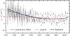 |
Fig. 2 30-day estimates of the Earth’s J2 values from satellite laser ranging (SLR) and its long term variation. The constant |

Weighted fits of straight lines and parabola to the J2 data from SLR.
It is important to mention that the J2 variation is a geophysical effect that cannot be predicted precisely by theories: only empirical models depending on observational data can be applied. Because of its important role in developing the precession model, we use the more realistic quadratic model of J2 variation to replace the classical linear model. The contribution of J2 variation to the precession rate in longitude (rψ in Eq. (12)) is listed in Table 6, where the deceleration term was not considered in the IAU solution. We mention that the J2 variation has no effect on the precession rate rϵ in obliquity.
3.2. Integration constants
The integration constants r0 and u0 at J2000.0 for precession rates in longitude and obliquity are crucial for solving the precession Eqs. (10) as they will be exactly the t1 terms ψ1 and ω1 in the final polynomials for the basic quantities ψA and ωA. Following the strategies of the P03 and P04 paper, we start to calculate the integration constants from the MHB2000 (Mathews et al. 2002) values for the corrections to the precession rates of IAU 1976.
In the MHB model, the corrections to the precession rates are derived from the VLBI fit of theoretical expressions for the precession rate and complex amplitude of a large amount of nutation terms to their observational estimates (or “input data”). In the original MHB2000 paper, the non-linear term P(nr) is −21 050 μas cy-1, introducing the correction in precession rate (we note that there is small inconsistency for the value between paragraph [70] and Table 7 in MHB2000 paper):  (14)and this value was adopted by the IAU 2006 model. Then the precession corrections used in the P04 model given in Capitaine et al. (2005) are compatible with the updated non-linear terms of −960 μas cy-1 in longitude and + 340 μas cy-1 in obliquity, which read
  (15)and the P04 model is based on this revised value of dMHBψ1.
According to Lambert & Mathews (2008) the precession corrections should, in principle, be consistent with the updated non-linear terms, that is, EL+AE+OT contributions of −124 μas cy-1 in longitude and + 1844 μas cy-1 in obliquity (item iv in Sect. 3.1). It requires a re-analysis of the MHB original VLBI data in MHB approach, which provide Basic Earth Parameters (BEPs) including the dynamical flattening Hd to give out the corrected precession rate (Herring et al. 2002). Since the detailed VLBI fits are far beyond the scope of our paper, we decide to keep the value in Eq. (15). This would be reasonable with no precision loss for the following two reasons: (1) the magnitude changes in the non-linear terms from P04 to this paper is about 25 times less than the magnitude from MHB to P04, which means that the change in the precession rate (relative to P04 value) would be much smaller for the current case (if the relation between the non-linear term and precession rate correction is rectilinear, the resulting value corresponding the new non-linear term is dMHBψ1 = −299 088 μas cy-1, which is very close to Eq. (15) within the 1σ uncertainty: this kind of estimate is just a test and will not be used); (2) we note that from the MHB to the P04 model, the precession corrections are consistent to within their standard errors although the difference between respective non-linear terms amounts to a considerable value of 20 100 μas cy-1. Therefore it is safe and reasonable to use Eq. (15) as the MHB correction to the precession rate: this keeps our solution dynamically consistent with the MHB and IAU 2006 models. The new MHB integration constants thus used in our calculation are such that 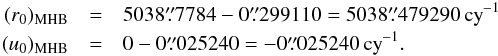 (16)The later expression for u0 is exactly the same as that in the IAU 2000 model (Mathews et al. 2002). The new non-linear contribution to the precession rates in longitude and obliquity in Lambert & Mathews (2008) will be applied as the theoretical contribution in the integration.
The non-ignorable spurious contributions to the MHB precession rates at J2000.0 were estimated in the IAU 2006 paper for the first time, including the “observed” effect resulting from the dependence of the VLBI observed precession rate in longitude on the chosen ecliptic (or the obliquity of epoch): 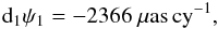 (17)and the effect of non-rigorous treatment of frame bias before 2003:
  (18)In the original P03 paper, d2ψ1 and d2ω1 were subtracted from the MHB estimates of the integration constants to derive the corrected precession rates:
 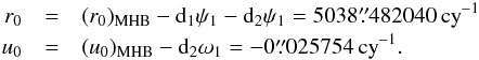 (19)In our computation, the numerical integration is carried out using the above r0 and u0 as integration constants. Another way of dealing with d2ψ1 and d2ω1 was suggested in the P04 paper (Capitaine et al. 2005), by which a new set of integration constants can be generated. The test of this problem with VLBI data is performed in Sect. 4.1.
3.3. Polynomial expressions for the precession of the equator
The upgraded precession of the equator is obtained by solving the differential Eqs. (10) by using (i) the updated ecliptic precession expressions derived from VSOP2013 and DE422 (cf. lines 1 and 3 in Table 3); (ii) the additional theoretical contributions to the precession rates described in Sect. 3.1; and (iii) integration constants r0 and u0 given in Eq. (19). The solutions for the basic precession quantities, ψA and ωA, for the updated solution (denoted LC solution) are such that  (20)with
  . The secondary quantities pA, ϵA, and χA are simultaneously derived as:
  (21)If the INPOP10a induced ecliptic precession (cf. lines 5 and 7 of Table 3) is used to replace the DE422 ecliptic in the integration, the resulting difference of ψA and ωA is (in μas)
  (22)This confirms that the effect of different ecliptic precessions is completely negligible.
Differences of the precession quantities between present solution LC and the IAU 2006 solution in the sense of Δ = [LC−IAU 2006].
The comparison of the LC solution with the IAU 2006 precession is shown in Table 7. The largest difference in the quadratic and cubic terms for ψA and pA is attributed to the use of updated empirical model for J2 variation. The signs for the t3 terms of ψA are now positive while in IAU 2006 they are negative. The precession in obliquity ωA is identical with that of the IAU 2006 because the integration constant for both cases is the same: the only difference for ωA at the order smaller than 1μas cy-1 originates from the ϵ-dependence of these new theoretical contributions. The deviations in parameters ϵA and χA result from both new ecliptic and equator precessions. The largest uncertainties in our solution for the precession in longitude are still attributed to the imperfect modeling of the J2 variation. Based on the fitted parameters in Table 5, the relative errors in linear and quadratic terms of rψ are as high as 40% and 18% (see Table 6), responsible for about 0.5 mas cy-2 and 4.5 mas cy-3 uncertainties in the t2 and t3 terms of ψA.
4. Comparison of the precession expressions with VLBI celestial pole offsets
The geodetic/astrometric VLBI technique plays a crucial role in understanding the Earth’s rotation. It monitors the celestial coordinates of the CIP and the Universal Time (UT1), which are known as the Earth orientation parameters (EOP). The current accuracy of VLBI observations is unprecedentedly high, namely at microarcsecond level, thus it provides the best observational material for studying the behavior of the precession-nutation models. As VLBI observations have shown that there are deficiencies in the IAU 2006/2000 model of the order of 0.2 mas, mainly due to the fact that the free core nutation (FCN) is not part of the model, the IERS will continue to publish observed estimates of the corrections to the IAU 2006/2000 precession-nutation. The observed differences with respect to the IAU-model-predicted CIP positions are reported as “celestial pole offsets” (CPO) dX and dY:  (23)the subscript “IAU” meaning that the reference model is the standard IAU 2006/2000AR06 precession-nutation model. Capitaine et al. (2009) applied several kinds of empirical models (linear, parabola, linear plus 18.6-yr nutation, and parabola plus 18.6-yr nutation) to fit the series of celestial pole offsets (1979–2008), in order to obtain the corrections for the IAU 2000 and IAU 2006/2000 precession-nutation models with respect to observations. In that work, there was an unexplained quadratic “curvature” in the residuals, which may be related to the Earth’s J2 rate uncertainty. We try to discuss this subject using the additional seven years of VLBI data (2009–2015) and the revised precession model LC.
To derive the celestial pole offsets with respect to the upgraded LC precession, we used the rigorous procedure as described in Capitaine (2006). First we evaluate the precession matrix  using the LC precession expressions:
  (24)where the parameters are given in Eqs. (20) and (21). This four-rotation transformation method makes use of the parameters that are derived directly from the dynamical solution and separates clearly the precession of the ecliptic and the equator. Then the nutation-precession-bias matrix ℳLC can be calculated using the IAU 2000AR06 nutation matrix
  and the frame bias matrix ℬ at J2000.0:
  (25)In the next step, the CIP coordinates corresponding the LC precession are extracted from the matrix ℳLC:
  (26)Finally, the theoretical predictions of XLC and YLC are subtracted from the observed position to obtain the new celestial pole offsets:
  (27)in which Xobs and Yobs are derived from Eq. (23). The above calculations are carried out using the SOFA software package (Standard of Fundamental Astronomy, IAU SOFA board 2014).
The time series for celestial pole offsets3 are shown in Fig. 3 and refer to the LC and IAU 2006 precessions respectively. The free core nutation has been removed with the empirical model of the IERS (Petit & Luzum 2010). Small curvatures can be seen from the time series of CPOs but the difference is not clearly distinguishable by the eye.
For each dX and dY time series, we calculated the weighted mean (WM) value and the weighted root mean square (prefit-WRMS) to indicate the overall consistency between the theoretical predictions and observations (see Table 8). Here the WRMS of an ensemble of data xi with standard errors σi is defined as:  (28)where
  is the classical weight.
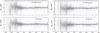 |
Fig. 3 Celestial pole offsets with respect to the LC and IAU 2006 precession expressions. The free core nutation (FCN) has been removed. |
Weight mean (WM) and weighted mean root square (WRMS) of the celestial pole offsets related to the LC, LC′, and the IAU 2006 precession models.
Integration constants and main contributions from first order terms of luni-solar torques correspond to P03-like and P04-like ways.
4.1. Test the validity of P03-like and P04-like integration constants
As mentioned in Sect. 3.2, spurious contributions to the MHB precession rates d1ψ1, d2ψ1, and d2ω1 (cf. Eqs. (17) and (18)) should be eliminated from (r0)MHB and (u0)MHB. However, the way to apply the effect of d2ψ1 and d2ω1 is controversial: the IAU 2006 (P03, Capitaine et al. 2003a) and later P04 model (Capitaine et al. 2005) applied these corrections with opposite signs. This caused a discrepancy of hundreds to one thousand microarcseconds per century in precession rates. We call the two conflicting approaches P03-like and P04-like. Our LC solution was computed using the P03-like method. We also tried to apply the P04-like integration constants as listed in Table 9 to derive a revised precession solution named LC′. All of the other details in the integration are exactly the same as in LC. According to the integration constants, the main contributions to precession rates (r0)1 and (u0)1 originate from the first order luni-solar terms and are also provided in this table, where (r0)th and (u0)th are the total theoretical contributions, for example, for the LC model,  and for the IAU 2006,
 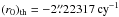 .
.
By integrating the precession equations, the primary parameters for the LC′ solution in longitude and obliquity are 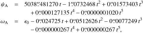 (29)with . Except for the linear terms, the difference larger than 1 μas between the LC and LC′ solutions only appears in the quadratic terms in longitude, and the differences in those terms can be written (in μas) as:
  (30)The VLBI time series corresponding to the LC′ precession are generated in the same way as for the LC solution, and the WM and WRMS values for this series are also presented in Table 8. This test can be presented as being an extension of the test of the P04 versus P03 solutions in Capitaine et al. (2005), with ten additional years of VLBI data. We note that the only difference between the LC and LC′ solution is that different integration constants (P03-like and P04-like) have been used. For the dX component, the WM and WRMS for both LC and LC′ solutions are smaller than the IAU 2006 values. Regarding the dY component, however, the WM and WRMS relative to the LC′ solution are even larger than the IAU model while the values relative to the LC solution are close to the IAU value, which means that the use LC′ precession solution deviates away from observations more than the other two models. In addition, we tried to integrate the precession equations with the IAU 2006 precession of the ecliptic and Earth model (theoretical contributions to the theoretical precession rates including J2 rate) but with P04 interpretation of integration constants r0 and u0 was:
 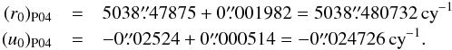 (31)The resulting precession expressions are also checked with the same method and VLBI time series. The relative WM and WRMS of the celestial pole offsets are not surprisingly larger than the IAU 2006 values in Table 8:
 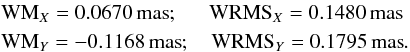 (32)This confirms that the implementation of corrections d2ψ1 and d2ω1 (Eq. (18)) to the integration constants should be identical to the P03/IAU 2006 model (P03-like approach). The above tests clearly allow us to conclude that the treatment of the integration constants in the LC solution is correct and that the P04-like case should be definitively eliminated. Therefore LC′ will not be considered in the rest of this paper. Only the LC solution is tested further.
4.2. Comparison of the IAU 2006 versus LC precession models with VLBI data
First, we can see from Table 8 that the smallest WM and WRMS of the celestial pole offsets can be found when the LC precession model has been used to calculate the CIP location. For the dX component, the LC solution appears to be more consistent with VLBI observations than the current IAU 2006 precession in the global sense, since the WM decreases by about 72% with reference to the IAU one.
To interpret more thoroughly the residuals between the observations and the two precession solutions, we have used (i) a parabola; (ii) a straight line plus 18.6-yr nutation; and (iii) a parabola plus the 18.6-yr nutation as in Capitaine et al. (2009) for the least squares fit. The 18.6-yr nutation is the largest nutation term and is expected to be sensitive to the errors of the secular precession model. The equations used for the fit of the celestial pole offsets are such that: 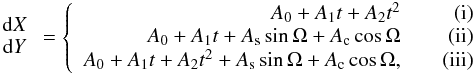 (33)where Ω (polynomial function of t) is the mean longitude of the ascending node of the Moon with a period of 6798.38 days (approximately equal to 18.6 yr).
The coefficients (A0,A1,A2,As,Ac) in the three functions of Eq. (33) are estimated from the weighted least squares fits and are listed in Table 10. It is clear that the longer time span of VLBI data reduced the coefficients of the quadratic model, especially the t2 term, compared to the results in Capitaine et al. (2009), indicating that the IAU 2006 precession is effective for predicting the CIP position. Furthermore, the coefficient of t2 term decreased significantly when the LC precession was adopted, but the signs are opposite to the IAU 2006 value. Since the most important change in the LC precession is the introduction of the updated J2 variation, which mainly modifies the quadratic and cubic terms of the precession in longitude, we have shown that the use of the J2 quadratic variation eliminated most of the residual quadratic curvature in the celestial pole offsets. This conclusion is consistent with previous checks by WM and WRMS. On the other hand, the resulting coefficients obtained from fitting linear plus 18.6-yr or parabola plus 18.6-yr periodic term differ significantly in each case. However, it is still difficult to discriminate which model is more appropriate to interpret the physical reason for the overall residuals because all of the post-fit WRMS in Table 8 reduced by approximately the same level. Another feature is the unstable t1 coefficients for the LC model that may be due to the large t3 term of ψA in the LC model (Eq. (29)).
Table 11 presents the correlation matrix of the coefficients in different empirical models. The elements in the upper triangular matrix correspond to the IAU 2006 precession while the low triangular matrix is for the LC solution. In the parabola model, the constant-quadratic and linear-quadratic correlation coefficients are up 0.7 for both precession models, showing that the VLBI residuals cannot be simply interpreted by quadratic function. This conclusion is similar to Capitaine et al. (2009). In the model comprising of the linear plus 18.6 yr periodic term, the correlation coefficients between linear and sine term for the IAU model is as high as 0.5, but it decreases to about 0.2 in the case of the LC precession. From Table 11 we can conclude that the linear plus 18.6 yr is better than the other two empirical models especially for the LC precession. For the parabola plus 18.6 yr periodic term, which was abandoned by Capitaine et al. (2009), the correlation coefficients for the updated LC model (mean absolute value of 0.19) are globally lower than the IAU model (mean absolute value of 0.42) except for the 0.7 correlation between A0 and A2. Indeed, the fit using the last empirical model leads to the reasonable inference that the quadric and period behaviors in the VLBI residuals become noticeable and separable with longer VLBI time series and the updated long-term variation of J2. The unexplained “curvature” in the residuals in previous studies (quite difficult to interpret in the past) may be expected to be modeled by a more realistic Earth model.
For the dY component, the fitted results (see Tables 10 and 11) are identical for the LC and the IAU model since the expressions for ωA are almost the same. The fitted coefficients reduced significantly with respect to Capitaine et al. (2009) thanks to the longer time span of the VLBI data.
Correlation matrix in the least squares fit for different empirical models.
5. Summary and discussion
In this work we have investigated the possibility of improving the IAU 2006 precession (Capitaine et al. 2003a) model with progress in the latest decade and an approach similar to the IAU 2006 method. The precession of the ecliptic has been derived using the latest analytical ephemerides VSOP2013 and numerical ephemerides DE422/INPOP10a. The polynomials for p and q provided by VSOP2013 are improved by fitting them to the DE422 and INPOP10a over 2000 yr centered on J2000.0. The resulting PA and QA differ from the IAU 2006 parameters by several tens of microarcseconds per century in secular terms, but this can be considered as negligible for the calculation of the precession of the equator. The differences in higher order terms are also too small to be considered.
The precession of the equator was obtained by solving the dynamical equations taking into account the revised precession of the ecliptic, the new theoretical contributions to the precession rates, and the updated integration constants. The progress in theoretical precession rates includes contributions from revised non-linear terms, tidal Poisson terms, second-order torque, Galactic aberration, and the most important new determination of the J2 variation. Based on the 35-year monitoring by the SLR, the long-term variations J2 appears to be more quadratic than linear in nature. This feature modified the quadratic and cubic terms in the precession in longitude ψA by about 5700 μas cy-2 and 16 800 μas cy-3, respectively. For the integration constants, we checked two interpretation of the correction from the non-rigorous treatment of bias and found that the approach used in the IAU 2006 model is correct: the P04-like approach should be eliminated. The LC solution is therefore recommended as the upgraded expression for the precession of the equator, but the accuracy of the updated precession is mainly restricted by the uncertainties in the J2 empirical model.
We have compared our solution to the IAU 2006 model with the most accurate VLBI series of celestial pole offsets. The weight mean and weighted root mean square values of the dX celestial pole offsets relative to the LC precession reduced by about 72% and 7%. The fits of different empirical models to the longer VLBI residuals have shown the different characteristics of the LC and IAU 2006 precession, mainly due to the adoption of a new J2 variation. The improvement in correlation coefficients implies that the linear plus 18.6 yr term is the most efficient. The model with parabola plus 18.6 yr term begins to be effective as more VLBI data are available, and it would be helpful for us to understand the long periodic signals in the VLBI residuals.
5.1. Choice of the standard precession model
The LC precession solution developed in this paper is based on recent improvements in EMB motion and theoretical contributions to precession. Our solution refined the IAU standard model to a certain extent and has potential to replace the IAU 2006 precession model in the future. However, at present, we recommend the continued use of the current IAU model for the following reasons: (i) the changes in the precession of the ecliptic can be considered as negligible; (ii) the J2 variation (which is the most important feature of the LC solution) can still be approximated by an empirical model with relatively large uncertainties but cannot be predicted by geophysical theories. In Cheng et al. (2013), new models for the J2 variations have been proposed but no model for the secular term is considered as being adopted by the geophysical community. Moreover, it is not possible to compare the validity of the corresponding quadratic terms in precession using only 35 yr of VLBI observations. An expression for has been proposed in this paper but this cannot be considered as providing a more accurate expression yet; (iii) improvement of the LC solution is not very convincing from the comparison with VLBI; (iv) the precession model itself is a secular phenomenon over tens of thousand years: ten years of progress seems insufficient to change the standard of the model; (v) the IAU 2006 precession is widely used by researchers in fundamental astronomy, especially in VLBI data reduction, and frequent change of the precession is not helpful for revealing the physical reason for its deficiency.
5.2. The role of the ecliptic and the future precession-nutation model of the Earth
After the adoption by the IAU of the International Celestial Reference System (ICRS) and new CIO-based parameterization for describing the Earth’s rotation, the problems concerning the role of the ecliptic in modern fundamental astronomy was proposed (Capitaine & Soffel 2015). To develop the precession of the equator, the conventional ecliptic was usually introduced as a reference plane to help the authors to write the simplified differential equations and apply the semi-analytical approach with precession rates provided by theories and observations. However, it should be remembered that the precession-nutation models describe the position of the Earth’s rotation pole (CIP) rather than the ecliptic pole in space, so that the ecliptic can, in principle, be abandoned in Earth rotation studies. For example, the CIO-based parameterization can be written without any concept of the ecliptic. We also note that the use of the ecliptic is not mandatory since the dynamical equations for the Earth’s rotation can be developed using directly the CIP coordinates X and Y (e.g., Capitaine et al. 2006), where the ecliptic was avoided. This subject will be discussed more deeply but it is clear that the role of the ecliptic will not be as crucial as it was in the past.
As for the future of the theory of the Earth’s rotation, the secular part, namely precession, and the periodic part, namely nutation, should be solved simultaneously to provide a self-consistent model (see e.g., Escapa et al. 2014). The VLBI will still be the main observational technique to refine the model of the Earth’s rotation. Furthermore, the use of the Gaia (Perryman et al. 2001) reference system will bring an opportunity to compare the precession-nutation in optical bandpass with that determined by VLBI at a homogeneous level of accuracy which could not be done in the past.
χA is also known as the precession of the ecliptic.
RKF is a single step integrator for the numerical solution of ordinary differential equations. RKF7(8) method is of order O(h7) with an error estimator of order O(h8), where h is length of step.
Solution derived at Paris Observatory, http://ivsopar.obspm.fr/nutation/geo.dat
Acknowledgments
This work is funded by the National Natural Science Foundation of China (NSFC) under grant Nos. 11303018 and 11473013 and the Natural Science Foundation of Jiangsu Province under No. BK20130546. The authors are grateful to the referee of this paper for his/her valuable suggestions to improve the text.
References
- Bretagnon, P., & Francou, G. 1988, A&A, 202, 309 [Google Scholar]
- Bretagnon, P., Rocher, P., & Simon, J.-L. 1998, A&A, 329, 329 [NASA ADS] [Google Scholar]
- Bretagnon, P., Fienga, A., & Simon, J.-L. 2003, A&A, 400, 785 [NASA ADS] [CrossRef] [EDP Sciences] [Google Scholar]
- Bourda, G., & Capitaine, N. 2004, A&A, 428, 691 [NASA ADS] [CrossRef] [EDP Sciences] [Google Scholar]
- Capitaine, N. 2012, Proc. Journées 2011, Systèmes de Référence spatio-temporels, eds. H. Schuh, S. Bohm, T. Nilsson, & N. Capitaine, Vienna University of Technology, 266 [Google Scholar]
- Capitaine, N., & Soffel, M. 2015, Proc. Journées 2014, Systèmes de Référence spatio-temporels, eds. Z. Malki, & N. Capitaine, Pulkovo observatory, 61 [Google Scholar]
- Capitaine, N., & Wallace, P. T. 2006, A&A, 450, 855 [NASA ADS] [CrossRef] [EDP Sciences] [Google Scholar]
- Capitaine, N., Wallace, P. T., & Chapront, J. 2003a, A&A, 412, 567 (IAU 2006/P03) [NASA ADS] [CrossRef] [EDP Sciences] [Google Scholar]
- Capitaine, N., Chapront, J., Lambert, S., & Wallace, P. T. 2003b, A&A, 400, 1145 [NASA ADS] [CrossRef] [EDP Sciences] [Google Scholar]
- Capitaine, N., Wallace, P. T., & Chapront, J. 2004, A&A, 421, 365 [NASA ADS] [CrossRef] [EDP Sciences] [Google Scholar]
- Capitaine, N., Wallace, P. T., & Chapront, J. 2005, A&A, 432, 355 (P04) [NASA ADS] [CrossRef] [EDP Sciences] [Google Scholar]
- Capitaine, N., Folgueira, M., & Souchay, J. 2006, A&A, 445, 347 [NASA ADS] [CrossRef] [EDP Sciences] [Google Scholar]
- Capitaine, N., Mathews, P. M., Dehant, V., Wallace, P. T., & Lambert, S. B. 2009, CeMDA, 103, 179 [Google Scholar]
- Cheng, M. K., & Tapley, B. D. 2004, J. Geophys. Res., 109, B009402 [NASA ADS] [CrossRef] [Google Scholar]
- Cheng, M. K., Tapley, B. D., & Ries, J. C. 2013, J. Geophys. Res., 118, 740 [NASA ADS] [CrossRef] [Google Scholar]
- Escapa, A., Getino, J., Ferrándiz, J. M., & Baenas, T. 2014, Proc. the Journées 2013, Systèmes de référence spatio-temporels, ed. N. Capitaine, Observatoire de Paris, 148 [Google Scholar]
- Fienga, A., Manche, H., Kuchynka, P., et al. 2010, ArXiv e-prints [arXiv:1011.4419v1] [Google Scholar]
- Fienga, A., Laskar, J., Kuchynka, P., et al., 2011, Celest. Mech. Dyn. Astr., 111, 363 [Google Scholar]
- Folgueira, M., Dehant, V., Lambert, S. B., & Rambaux, N. 2007, A&A, 469, 1197 [NASA ADS] [CrossRef] [EDP Sciences] [Google Scholar]
- Folkner, W. M., Williams, J. G., & Boggs, D. H. 2008, JPL Memorandum IOM 343R-08-003 [Google Scholar]
- Fukushima, T. 2003, AJ, 126, 494 [NASA ADS] [CrossRef] [Google Scholar]
- Gerlach, E., Klioner, S., & Soffel, M. 2012, ArXiv e-prints [arXiv:1202.5870v1] [Google Scholar]
- Harada, W., & Fukushima, T. 2004, AJ, 127, 531 [NASA ADS] [CrossRef] [Google Scholar]
- Herring, T. A., Mathews, P. M., & Buffett, B. A. 2002, J. Geophys. Res., 107, 4 [Google Scholar]
- Hilton, J. L., Capitaine, N., Chapront, J., et al. 2006, Celest. Mech. Dyn. Astron., 94, 351 [NASA ADS] [CrossRef] [Google Scholar]
- IAU SOFA Board, IAU SOFA Software Collection, Issue 2013-12-02, available at http://www.iausofa.org [Google Scholar]
- Lambert, S. B., & Mathews, P. M. 2006, A&A, 453, 363 [NASA ADS] [CrossRef] [EDP Sciences] [Google Scholar]
- Lambert, S. B., & Mathews, P. M. 2008, A&A, 481, 883 [NASA ADS] [CrossRef] [EDP Sciences] [Google Scholar]
- Lieske, J. H., Lederle, T., Fricke, W., & Morando, B. 1977, A&A, 58, 1 (IAU 1976) [NASA ADS] [Google Scholar]
- Liu, J.-C., Capitaine, N., Lambert, S. B., Malkin, Z., & Zhu, Z. 2012, A&A, 548, A50 [NASA ADS] [CrossRef] [EDP Sciences] [Google Scholar]
- Luzum, B., Capitaine, N., Fienga, A., et al. 2011, Celest. Mech. Dyn. Astron., 110, 293 [NASA ADS] [CrossRef] [Google Scholar]
- Mathews, P. M., Herring, T. A., & Buffett, B. A. 2002, J. Geophys. Res., 107, 4 [Google Scholar]
- Nerem, R. S., Chao, B. F., Au, A. Y., et al. 1993, Geophys. Res. Lett., 20, 595 [Google Scholar]
- Perryman, M. A. C., de Boer, K. S., Gilmore, G., et al. 2001, A&A, 369, 339 [NASA ADS] [CrossRef] [EDP Sciences] [Google Scholar]
- Petit, G., & Luzum, B. 2010, IERS Conventions (2010), IERS Technical Note No. 36 [Google Scholar]
- Simon, J.-L., Francou, G., Fienga, A., & Manche, H. 2013, A&A, 557, A49 [NASA ADS] [CrossRef] [EDP Sciences] [Google Scholar]
- Standish, E. 1998, JPL Interoffice Memorandum, 312, 98 [Google Scholar]
- Stephenson, E. R., & Morrison, L. V. 1995, Philos. Trans. R. Soc. London, Ser. A, 351, 165 [Google Scholar]
- Williams, J. G. 1994, AJ, 108, 711 [NASA ADS] [CrossRef] [Google Scholar]
- Yoder, C. F., Williams, J.-G., Dickey, O., et al. 1983, Nature, 303, 757 [Google Scholar]
All Tables
Equator to Ecliptic coordinate system transformation angles for DE422 and INPOP10a.
Precession quantities of the ecliptic derived from VSOP2013 and DE422/INPOP10a ephemerides and comparison with the IAU 2006 model.
Values of J2 rate estimated by observations or adopted in the IAU 2006 precession.
Differences of the precession quantities between present solution LC and the IAU 2006 solution in the sense of Δ = [LC−IAU 2006].
Weight mean (WM) and weighted mean root square (WRMS) of the celestial pole offsets related to the LC, LC′, and the IAU 2006 precession models.
Integration constants and main contributions from first order terms of luni-solar torques correspond to P03-like and P04-like ways.
All Figures
|
Fig. 1 Difference of PA and QA between various ephemerides used in this paper over 20 centuries (1000−3000). A different scale is used in the bottom plot (d). |
| In the text | |
|
Fig. 2 30-day estimates of the Earth’s J2 values from satellite laser ranging (SLR) and its long term variation. The constant |
| In the text | |
|
Fig. 3 Celestial pole offsets with respect to the LC and IAU 2006 precession expressions. The free core nutation (FCN) has been removed. |
| In the text | |
Current usage metrics show cumulative count of Article Views (full-text article views including HTML views, PDF and ePub downloads, according to the available data) and Abstracts Views on Vision4Press platform.
Data correspond to usage on the plateform after 2015. The current usage metrics is available 48-96 hours after online publication and is updated daily on week days.
Initial download of the metrics may take a while.