| Issue |
A&A
Volume 596, December 2016
|
|
|---|---|---|
| Article Number | A41 | |
| Number of page(s) | 5 | |
| Section | The Sun | |
| DOI | https://doi.org/10.1051/0004-6361/201629209 | |
| Published online | 28 November 2016 | |
Suprathermal electron distributions in the solar transition region
1 Leibniz-Institut für Astrophysik Potsdam, An der Sternwarte 16, 14482 Potsdam, Germany
e-mail: This email address is being protected from spambots. You need JavaScript enabled to view it.
2 Astronomical Institute of the Academy of Sciences of the Czech Republic, Fricova 298, 251 65 Ondrejov, Czech Republic
Received: 29 June 2016
Accepted: 2 October 2016
Abstract
Context. Suprathermal tails are a common feature of solar wind electron velocity distributions, and are expected in the solar corona. From the corona, suprathermal electrons can propagate through the steep temperature gradient of the transition region towards the chromosphere, and lead to non-Maxwellian electron velocity distribution functions (VDFs) with pronounced suprathermal tails.
Aims. We calculate the evolution of a coronal electron distribution through the transition region in order to quantify the suprathermal electron population there.
Methods. A kinetic model for electrons is used, which is based on solving the Boltzmann-Vlasov equation for electrons including Coulomb collisions with both ions and electrons. Initial and chromospheric boundary conditions are Maxwellian VDFs with densities and temperatures based on a background fluid model. The coronal boundary condition has been adopted from earlier studies of suprathermal electron formation in coronal loops.
Results. The model results show the presence of strong suprathermal tails in transition region electron VDFs, starting at energies of a few 10 eV. Above electron energies of 600 eV, electrons can traverse the transition region essentially collision-free.
Conclusions. The presence of strong suprathermal tails in transition region electron VDFs shows that the assumption of local thermodynamic equilibrium is not justified there. This has a significant impact on ionization dynamics, as is shown in a companion paper.
Key words: Sun: transition region / plasmas / methods: numerical
© ESO, 2016
1. Introduction
Suprathermal tails are a commom feature of solar wind electron velocity distribution functions (VDFs). Lin (1998) has identified different components, a thermal core, an extended suprathermal halo, and a superhalo with energies up to tens of keV. Maksimovic et al. (1997) have shown that kappa distributions provide better fits to solar wind suprathermal electron VDFs than sums of Maxwellian distributions. Kappa distributions can also be considered as equilibrium states in non-extensive statistical mechanics (Leubner 2004; Livadiotis & McComas 2013).
While direct observations of suprathermal electron VDFs are only possible in situ in the solar wind, several models predict a coronal origin. They are, for example, based on coronal turbulence (Roberts & Miller 1998), obliquely propagating finite-amplitude electromagnetic waves (Viñas et al. 2000), or nanoflares (Che & Goldstein 2014). In the corona, a suprathermal electron population can lead to non-local effects through velocity filtration, including heat fluxes against a temperature gradient (Scudder 1992a,b). The existence of suprathermal electrons corresponds to plasma states away from thermal equilibrium, whose influence on ion charge states has been discussed by Cranmer (2014), and for the solar wind model of Pierrard & Pieters (2014).
Vocks et al. (2005) have developed an electron kinetic model for the solar wind that aims at understanding the formation of a suprathermal electron component from an initially Maxwellian distribution through resonant interaction with a given whistler wave spectrum. It is based on solving the Boltzmann-Vlasov equation, including the effects of Coulomb collisions and resonant electron – whistler wave interaction. The wave spectrum has been chosen as a power law representing the high-frequency tail of wave spectra associated with coronal heating. The results showed that such a set-up indeed leads to the formation of suprathermal tails in the electron VDF as a by-product of coronal heating.
Vocks et al. (2008) applied the same model on the closed volume of a coronal loop in order to better understand the suprathermal tail formation, without the open boundary conditions of the outer heliosphere. Indeed, they showed that power law-like electron VDFs are formed in the keV energy range. This loop model covers only a spatial domain with relatively high transition region temperatures near the loop footpoints; the actual transition region was largely excluded. This was necessary in order to avoid excessive computer costs associated with small electron thermal speeds and strong spatial density and temperature gradients there. These simulations confirmed that the quiet solar corona is capable of producing a substantial suprathermal electron population.
The hot corona and the cool chromosphere are only separated by a thin transition region. Coronal suprathermal electrons are not supposed to stop there. Owing to the v4-dependence of Coulomb collisional mean free paths on electron speed, v, electrons with sufficiently high energy are capable of traversing the transition region and even entering the cooler and denser chromosphere.
In this paper, we investigate how such suprathermal electrons propagate from the corona through the transition region into the chromosphere. The expectation that suprathermal electrons from the corona can cross the transition region towards the chromosphere, combined with the strong temperature gradient of the transition region, leads to the expectation that transition region electron VDFs can substantially deviate from Maxwellians.
We investigate the evolution of an electron VDF through the strong temperature gradient of the transition region. The results of this study can be used as input to calculate ionization states of transition region ions. The extent and the implications of this influence of suprathermal electrons on transition region ions, e.g. concerning the analysis of extreme UV (EUV) spectra, will be discussed in a companion paper.
2. The model
The electron kinetic model used here is based on the coronal loop model of Vocks et al. (2008). This is a Boltzmann-Vlasov code, including Coulomb collisions with both electrons and ions, and resonant interaction with whistler waves. The assumption of gyrotropic electron VDFs not only reduces the number of velocity coordinates from 3 to 2, but also eliminates the spatial coordinates perpendicular to the background magnetic field. Only the spatial coordinate along a magnetic field line needs to be considered.
The simulation box is now located just below the loop model of Vocks et al. (2008). So the new model is an extension of the old one, with a simple simulation box that covers the transition region and the uppermost chromosphere. Owing to its small spatial scale, the magnetic field topology and its spatial variation do not need to be considered here. The spatial coordinate of the simulation box is just oriented in the vertical direction, for a constant magnetic field. Its field strength is the same 136 G as for the old model loop footpoint, but the actual value has no influence on the results of the new model.
Resonant interaction with whistler waves is also not considered here; the “frequency sweeping” mechanism (Tu & Marsch 1997; Vocks & Mann 2003) would require a magnetic field variation along the spatial coordinate. Furthermore, this paper is focused on propagation effects of suprathermal electrons in the transition region, and the influence of Coulomb collisions on electron VDFs in cooler and denser solar atmospheric regions. The kinetic model is based on calculating the temporal evolution of the electron VDF, using the Boltzmann-Vlasov equation, ![Mathematical equation: \begin{equation} \frac{\partial f}{\partial t} + (\vec{v} \cdot \nabla) f + \left[m_{\rm e} \gamma \vec{g} - e (\vec{E} + \vec{v}\times\vec{B} \right] \cdot \frac{\partial f}{\partial \vec{p}} = \left(\frac{\delta f}{\delta t}\right)_\mathrm{coll}\!, \label{eq_vlasov} \end{equation}](/articles/aa/full_html/2016/12/aa29209-16/aa29209-16-eq3.png) (1)until a final steady state has been reached. The parameters g and E represent respectively the gravitational and charge separation electric field, B is the background magnetic field,
(1)until a final steady state has been reached. The parameters g and E represent respectively the gravitational and charge separation electric field, B is the background magnetic field, 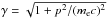 is the Lorentz factor, e is the elementary charge, and me is the electron rest mass. The term on the right-hand side represents the Coulomb collisions. This Vlasov kinetic electron model requires a background model for the ions, and also for the electrons as an initial condition inside the simulation box. A transition region temperature profile needs to be prepared and hydrostatic equilibrium then provides a density model. Since there are no heat sources or sinks in the model, a constant heat flux has to be assumed. The classic Spitzer T5/2 law of thermal conductivity in a plasma then leads to the following temperature profile in a plasma slab,
 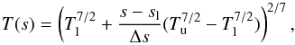 (2)with Tl and Tu as lower (chromospheric) and upper (coronal) boundary temperatures, sl as the location of the border between the chromosphere and the transition region, and Δs as the transition region thickness. This leads to a steep temperature gradient at low temperatures. Below the transition region, the chromospheric temperature profile from Fig. 3 of Gary et al. (2007) has been adopted, which is based on data from Peter (2001). The lower boundary of the simulation box is located in the uppermost chromosphere, so just the temperature there and the height of the transition region temperature jump had to be copied. The spatial scale of the model transition region from the chromosphere, with Tl = 1.1 × 10⁴ K, to a coronal temperature level, Tu = 1.4 × 10⁶ K, is set to Δs = 500 km.
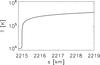 |
Fig. 1 Temperature profile of the transition region background model. |
Figure 1 shows the resulting transition region temperature profile. An extreme temperature gradient can be seen at lower temperatures, just above the chromosphere, with temperature changes of the order of 104 K on just a few meters. According to Lie-Svendsen et al. (1999), however, the classical heat flux law is still applicable in the strong temperature gradient of the transition region, although the presence of a strong enough suprathermal electron population can lead to deviations from classical Spitzer conductivity (Dorelli & Scudder 1999; Landi & Pantellini 2001; Dorelli & Scudder 2003).
The initial condition for solving the Boltzmann-Vlasov Eq. (1) is then provided by Maxwellian VDFs based on the temperatures and densities of the background model inside the simulation box. The kinetic model also needs given values for the electron VDF at the spatial boundaries of the simulation box. For the lower boundary, this is just a Maxwellian VDF with the density and temperature of the background model. For the upper boundary, the resulting VDF from the loop model of Vocks et al. (2008) with its suprathermal tail is used. The downward-propagating part of the electron VDF at the footpoint of the loop model is used as the upper boundary condition for the transition region model presented here.
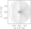 |
Fig. 2 Electron VDF at the upper boundary of the simulation box. The isolines are chosen in such a way that they form equidistant circles for a Maxwellian VDF. A coronal temperature of T = 1.4 × 10⁶ K corresponds to a thermal momentum |
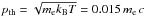
This electron VDF is displayed in Fig. 2. The downward moving (p∥< 0) electron population with a strong suprathermal tail can be seen. The elongated shape of the VDF is the result of suprathermal electron production by resonant interaction with whistler waves, as discussed in Vocks et al. (2008). The reason for the strong phase-space gradient near p∥ = 0 is that in the model of Vocks et al. (2008), this VDF was obtained as result near the loop footpoint where a Maxwellian VDF was provided as a boundary condition entering the loop (p∥> 0). This is not relevant here, since these electrons are not entering the transition region simulation box.
 |
Fig. 3 Electron VDFs parallel (solid line) and perpendicular (dotted line) to the spatial coordinate, and Maxwellian VDF (dashed line) for reference. |
Figure 3 shows cuts through the upper boundary electron VDF, both parallel and perpendicular to the background magnetic field, i.e. the spatial coordinate in vertical direction. For the parallel direction, p∥< 0 is plotted. The comparison with a Maxwellian VDF demonstrates the increase in electron fluxes between p = 0.05 mec and p = 0.2 mec, which corresponds to electron energies of 0.6−10 keV. These are the suprathermal electrons that enter the transition region simulation box.
3. Resulting electron VDF inside the transition region
After the preparation of initial and boundary conditions, the Boltzmann-Vlasov Eq. (1) is used to calculate the temporal evolution of the electron VDF inside the simulation box until a final steady state has been reached. A simulation time of 0.1 s is sufficient. It allows even chromospheric thermal electrons to traverse the simulation box multiple times.
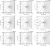 |
Fig. 4 Electron VDFs for nine different transition region temperature levels, displayed as in Fig. 2. |
Figure 4 shows the resulting transition region electron VDFs for nine different temperature levels. The background temperatures also become apparent as sizes of the thermal cores of the VDFs. Owing to the v-3-scaling of Coulomb collision frequencies with electron speed, v, the cores are collision-dominated, and the VDFs there quickly approach the Maxwellians of the background model. On the other hand, the overall shapes of the VDFs hardly change at higher energies, which is to be expected from the longer collisional mean free paths there.
For a better assessment of the suprathermal electron population, the VDFs can be pitch-angle averaged. Figure 5 shows plots of the resulting phase space densities for the same nine transition region temperature levels. Maxwellian VDFs with the same background densities and temperatures are plotted as dashed lines for reference. For a better comparison of VDFs with different background densities and temperatures, the plotted values are not normalized but are shown in absolute units (kg-3 m-6 s3).
An electron momentum of p = 0.1 mec corresponds to a kinetic energy of 2.5 keV. The energy range of the suprathermal electrons shown here therefore covers a few tens of eV up to a few keV.
It can be seen that the phase-space densities are the same for all temperature levels above an electron momentum of p = 0.05 mec, which corresponds to an energy of 640 eV. These electrons are essentially collision-free in the transition region, and can traverse it unaffected. For lower energies, the electron VDFs change with background temperature, as Coulomb collisions bring them closer to their respective Maxwellians. But even down to an electron momentum of p = 0.01 mec (25 eV), all lines are relatively close to each other.
The line for the lowest temperature of 12 000 K, which already corresponds to the upper chromosphere, is noteworthy. The phase-space density is significantly lower above p = 0.01 mec (25 eV) than for the next higher temperature level, which is spatially very close (see Fig. 1). Here, the rapid absorption of low-energy electrons in the cool and dense chromospheric plasma becomes evident.
This change in the VDF through the transition region leads to an evolution of the relative strength of the suprathermal tails as compared to the background density. The fraction of electrons with momentum greater than 3 times the thermal momentum, p> 3pth, with  , is displayed in Fig. 6. With decreasing temperature within the transition region, this fraction first increases. This is due to the small change in the VDF at suprathermal energies that was noted above, combined with a decreasing temperature, which lowers pth, so that a larger fraction of the phase space is considered “suprathermal”.
In the lower transition region, however, at temperatures below 50 000 K, this trend reverses. A local maximum is reached, with 4.2% of the electrons being in the suprathermal tail of the VDF. Towards the chromosphere this fraction decreases rapidly and approaches 2.5%. This is close to the value of 2.9% that corresponds to an isotropic Maxwellian VDF. The slight deviation from this value is due to the anisotropy of the VDF that is visible in Fig. 4. This decrease is the consequence of the rapid absorption of low-energy electrons at energies below 25 eV which can be seen in Fig. 5 for the lowest temperature. The remaining suprathermal tail of the VDF at energies above 25 eV does not contribute significantly to the fraction Nsuprathermal shown in Fig. 6.
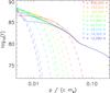 |
Fig. 5 Pitch-angle averaged electron VDFs for different transition region temperature levels (solid lines), and background Maxwellian VDFs (dashed lines). |
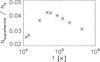 |
Fig. 6 Fraction of suprathermal electrons with momentum exceeding 3 × the thermal momentum, as a function of transition region temperature. |
4. Influence of the transition region background model
The strong absorption of electrons in the energy range of a few 10 eV indicates that the thickness of the model transition region itself may have a strong influence on the resulting suprathermal electron fluxes. In order to investigate this, we run a second simulation with a slightly modified model transition region with a flatter temperature profile. It is based on exponents 5/2 rather than 7/2 (Eq. (2)), as if the plasma thermal conductivity scales as T3/2. This choice is arbitrary, although it corresponds to the neutral hydrogen thermal conductivity that contributes to the thermal structure of the chromosphere and lowest transition region at temperatures T< 1.5 × 10⁴ K (McClymont & Canfield 1983).
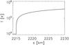 |
Fig. 7 Temperature profile of the modified transition region background model. |
The model transition region is now much thicker, see Fig. 7.
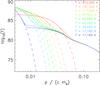 |
Fig. 8 Pitch-angle averaged electron VDFs for different transition region temperature levels (solid lines), and background Maxwellian VDFs (dashed lines), for the modified transition region temperature profile. |
Figure 8 shows the resulting pitch-angle averaged transition region electron VDFs for similar temperature levels as in the previous section. The comparison with the earlier results shows little difference for higher electron momentum above p = 0.05 mec (640 eV), but for lower energies the phase-space densities are substantially lower and stay close to their respective Maxwellian cores. This shows that the transition region model thickness has a strong influence on suprathermal electron fluxes in the energy range of a few 100 eV. Because of the v4-dependence of Coulomb collisional mean free paths, a thicker transition region allows for the absorption of suprathermal electrons with lower speed.
5. Discussion and summary
Our kinetic model results demonstrate that electron VDFs in the transition region are far away from a local thermodynamic equilibrium state with a Maxwellian VDF. There are strong fluxes of suprathermal electrons from the corona which can traverse the transition region essentially collision-free at energies above 600 eV.
The details of such transition region suprathermal electron fluxes depend on the coronal electron VDF, but even without a suprathermal electron population there, the coronal temperature of 1.4 × 10⁶ K can be expected to lead to suprathermal tails in transition region electron VDFs.
It has been found that the transition region electron phase-space density surpasses that of a Maxwellian for energies of a few 10 eV and above. This energy range is crucial for the ionization dynamics and EUV line formation in the transition region.
The exact values of phase-space densities, and therefore electron fluxes, depend on the transition region model. A thicker transition region leads to more suprathermal electron absorption, especially in the energy range up to a few 100 eV. However, the general result is model-independent: transition region electron VDFs show significant suprathermal tails; they are far away from a Maxwellian except for the collision-dominated thermal core.
This can have significant influence on the analysis of EUV data. A study of the impact of the suprathermal electron population on transition region ionization dynamics is presented in a companion paper (Dzifčáková et al. 2016).
Acknowledgments
The authors benefited greatly from participation in the International Team 276 funded by the International Space Science Institute (ISSI) in Bern, Switzerland. E.D. was supported by the Grant Agency of the Czech Republic under Grant No. P209/12/1652.
References
- Che, H., & Goldstein, M. L. 2014, ApJ, 795, L38 [NASA ADS] [CrossRef] [Google Scholar]
- Cranmer, S. R. 2014, ApJ, 791, L31 [NASA ADS] [CrossRef] [Google Scholar]
- Dorelli, J. C., & Scudder, J. D. 1999, Geophys. Res. Lett., 26, 3537 [NASA ADS] [CrossRef] [Google Scholar]
- Dorelli, J. C., & Scudder, J. D. 2003, J. Geophys. Res. (Space Phys.), 108, 1294 [NASA ADS] [CrossRef] [Google Scholar]
- Dzifčáková, E., Vocks, C., & Dudík, J. 2016, A&A, accepted [Google Scholar]
- Gary, G. A., West, E. A., Rees, D., et al. 2007, A&A, 461, 707 [NASA ADS] [CrossRef] [EDP Sciences] [Google Scholar]
- Landi, S., & Pantellini, F. G. E. 2001, A&A, 372, 686 [NASA ADS] [CrossRef] [EDP Sciences] [Google Scholar]
- Leubner, M. P. 2004, ApJ, 604, 469 [NASA ADS] [CrossRef] [Google Scholar]
- Lie-Svendsen, Ø., Holzer, T. E., & Leer, E. 1999, ApJ, 525, 1056 [NASA ADS] [CrossRef] [Google Scholar]
- Lin, R. P. 1998, Space Sci. Rev., 86, 61 [NASA ADS] [CrossRef] [Google Scholar]
- Livadiotis, G., & McComas, D. J. 2013, Space Sci. Rev., 175, 183 [NASA ADS] [CrossRef] [Google Scholar]
- Maksimovic, M., Pierrard, V., & Riley, P. 1997, Geophys. Res. Lett., 24, 1151 [NASA ADS] [CrossRef] [Google Scholar]
- McClymont, A. N., & Canfield, R. C. 1983, ApJ, 265, 483 [NASA ADS] [CrossRef] [Google Scholar]
- Peter, H. 2001, A&A, 374, 1108 [NASA ADS] [CrossRef] [EDP Sciences] [Google Scholar]
- Pierrard, V., & Pieters, M. 2014, J. Geophys. Res. (Space Phys.), 119, 9441 [Google Scholar]
- Roberts, D. A., & Miller, J. A. 1998, Geophys. Res. Lett., 25, 607 [NASA ADS] [CrossRef] [Google Scholar]
- Scudder, J. D. 1992a, ApJ, 398, 299 [NASA ADS] [CrossRef] [Google Scholar]
- Scudder, J. D. 1992b, ApJ, 398, 319 [NASA ADS] [CrossRef] [Google Scholar]
- Tu, C.-Y., & Marsch, E. 1997, Sol. Phys., 171, 363 [NASA ADS] [CrossRef] [Google Scholar]
- Viñas, A. F., Wong, H. K., & Klimas, A. J. 2000, ApJ, 528, 509 [NASA ADS] [CrossRef] [Google Scholar]
- Vocks, C., & Mann, G. 2003, ApJ, 593, 1134 [NASA ADS] [CrossRef] [Google Scholar]
- Vocks, C., Salem, C., Lin, R. P., & Mann, G. 2005, ApJ, 627, 540 [NASA ADS] [CrossRef] [Google Scholar]
- Vocks, C., Mann, G., & Rausche, G. 2008, A&A, 480, 527 [NASA ADS] [CrossRef] [EDP Sciences] [Google Scholar]
All Figures
|
Fig. 1 Temperature profile of the transition region background model. |
| In the text | |
|
Fig. 2 Electron VDF at the upper boundary of the simulation box. The isolines are chosen in such a way that they form equidistant circles for a Maxwellian VDF. A coronal temperature of T = 1.4 × 10⁶ K corresponds to a thermal momentum |
| In the text | |
|
Fig. 3 Electron VDFs parallel (solid line) and perpendicular (dotted line) to the spatial coordinate, and Maxwellian VDF (dashed line) for reference. |
| In the text | |
|
Fig. 4 Electron VDFs for nine different transition region temperature levels, displayed as in Fig. 2. |
| In the text | |
|
Fig. 5 Pitch-angle averaged electron VDFs for different transition region temperature levels (solid lines), and background Maxwellian VDFs (dashed lines). |
| In the text | |
|
Fig. 6 Fraction of suprathermal electrons with momentum exceeding 3 × the thermal momentum, as a function of transition region temperature. |
| In the text | |
|
Fig. 7 Temperature profile of the modified transition region background model. |
| In the text | |
|
Fig. 8 Pitch-angle averaged electron VDFs for different transition region temperature levels (solid lines), and background Maxwellian VDFs (dashed lines), for the modified transition region temperature profile. |
| In the text | |
Current usage metrics show cumulative count of Article Views (full-text article views including HTML views, PDF and ePub downloads, according to the available data) and Abstracts Views on Vision4Press platform.
Data correspond to usage on the plateform after 2015. The current usage metrics is available 48-96 hours after online publication and is updated daily on week days.
Initial download of the metrics may take a while.