| Issue |
A&A
Volume 596, December 2016
|
|
|---|---|---|
| Article Number | A18 | |
| Number of page(s) | 5 | |
| Section | Planets and planetary systems | |
| DOI | https://doi.org/10.1051/0004-6361/201527397 | |
| Published online | 22 November 2016 | |
Estimation of emission cone wall thickness of Jupiter’s decametric radio emission using stereoscopic STEREO/WAVES observations
1 Space Research Institute, Austrian Academy of Sciences, Schmiedlstrasse 6, 8042 Graz, Austria
e-mail: This email address is being protected from spambots. You need JavaScript enabled to view it.
2 Commission for Astronomy, Austrian Academy of Sciences, Schmiedlstrasse 6, 8042 Graz, Austria
e-mail: This email address is being protected from spambots. You need JavaScript enabled to view it.
Received: 18 September 2015
Accepted: 8 September 2016
Abstract
Aims. Stereoscopic observations by the WAVES instrument onboard two STEREO spacecraft have been used with the aim of estimating wall thickness of an emission cone of Jovian decametric radio emission (DAM).
Methods. Stereoscopic observations provided by STEREO-A and -B facilitate unambiguous recognition of the Jovian DAM in observed dynamic spectra as well as identification of its components (Io DAM or non-Io DAM). The dynamic spectra of radio emissions recorded by STEREO/WAVES have been analyzed using the method of cross-correlation of the radio dynamic spectra.
Results. Altogether, 139 radio events, in particular 91 Io- and 48 non-Io-related radio events were observed. The averaged width of the emission cone wall for Io-DAM as well as for non-Io DAM is about 1.1° ± 0.2°. These results are in agreement with previous findings.
Key words: planets and satellites: individual: Jupiter / masers / radiation mechanisms: non-thermal
© ESO, 2016
1. Introduction
Decametric radio emission (DAM) is the strongest component of Jovian radiation discovered over 60 years ago by Burke & Franklin (1955). This emission is observed in the form of arc-shaped radio bursts (on a timescale of minutes) in a frequency range from a few MHz up to 40 MHz (Carr et al. 1983; Zarka 1998). Observations of DAM are in agreement with the theory of cyclotron maser instability (CMI) in which the radiation is generated by accelerated electrons characterized by an instable distribution function, for example loss cone or shell distributions (Wu & Lee 1979; Treumann 2006).
A theory of the Jovian DAM, confirmed by the existing observations, predicts that Io-DAM emission radiates in a thin-walled hollow emission cone with the apex anchored at the instant magnetic field line at altitudes where the local electron gyrofrequency is close to the frequency of the observed radiation (Goldstein & Thieman 1981). Lecacheux et al. (1998) failed to model observed arc-shaped patterns of Io-DAM with the hollow cone beamed radio emission assuming that average half-apex angle is constant at all frequencies. At the same time, Queinnec & Zarka (1998) proposed that the half-apex angle of the hollow emission cone depends on the frequency. Later Hess et al. (2008) and Ray & Hess (2008) showed that within the CMI theory driven by, for example, loss-cone distribution, the beam angle is mainly defined by the velocity of the emitting electrons, and thus it indeed varies with the frequency. Additionally, Hess et al. (2008), Ray & Hess (2008) and Hess et al. (2010) successfully model the observed Jovian Io-DAM arcs using the ExPRES code. These simulations show that the arc-shaped patterns are strongly controlled by frequency dependent beam angle, lead angle, width of beaming cone wall and topology of the active magnetic field line relative to the observer.
An accurate description of instantaneous beaming properties of the arc-like Jovian radio emission is an important task for understanding the physical conditions in the emitting sources and radiation propagation. The CMI mechanism predicts that the maximum of growth rate of radiation is reached for propagation nearly perpendicular to the magnetic field in a narrow range of beaming angles, for example, Zarka et al. (1986). Therefore, the thickness of the wall of emission cone is an important parameter that describes the radiation properties of the Jovian DAM.
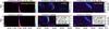 |
Fig. 1 Identification of the radio emission observed stereoscopically by STEREO/WAVES. Panel a) shows the solar type III radio burst observed simultaneously (dt ≈ 0) by STEREO-A (STA) and STEREO-B (STB). Panels b) and c) display examples of the DAM emission. The radiation on panel b) was observed sequentially by both spacecraft with time delay (dt ≈ 0.71 h) which corresponds to ≈ 26° of Jupiter’s rotation and ≈ 6.0° of the Io angular shift along its orbit. Since the angular separation between both spacecraft as seen from Jupiter was ≈ 6.3° we conclude that the observed radio emission is Io related DAM (see Sect. 2). Panel c) illustrates the identification of non-Io DAM. The spectra in b) and c) are plotted with a correction for difference in light travel time from Jupiter to each of the spacecraft. |
The first estimation of the emission cone wall thickness was based on the measurements on the duration of a given DAM arc at fixed frequency. Boischot et al. (1981) indicated that non-Io related arcs of DAM observed by Voyager/PRA had an average duration of 3−6 min that corresponds to 2°−4° of Jupiter rotation. Queinnec & Zarka (1998) and Zarka et al. (1997) estimated the thickness of the emission wall to be 1°−2°, equating the duration of Io-DAM arcs with period of the Io flux tube.
The other method of determination of the thickness of the hollow cone uses the stereoscopic observations of the Jovian radio emission by two (or more) spacecraft positioned at different Jovian longitudes. In this case both spacecraft can observe the same DAM arcs simultaneously (after correction for light travel time differences), but only when their longitudinal separation, as seen from Jupiter, is equal or less than the thickness of the emission cone. Kaiser et al. (2000) determine the thickness of the hollow cone wall of the DAM emission to be 1.5° ± 0.5°, using the stereoscopic observations of the Jovian radio emission from Wind and Cassini. These measurements were based on the limited number of stereoscopic observations and it was difficult to draw general conclusions regarding the width of the emission cone wall.
The angular separation between the two STEREO spacecraft, orbiting the Sun approximately twice per year is less than a few degrees. Therefore, the method described in Kaiser et al. (2000) has been applied to determine the statistically confident results of the beaming width of the Io and non-Io DAM observed during the years 2007−2014. Altogether 139 radio episodes, in particular 91 Io- and 48 non-Io-related radio events have been analyzed. We have determined the averaged width of the emission cone wall for Io- and non-Io events using the cross-correlation analysis.
2. Observations and identification of DAM emission in STEREO/WAVES dynamic spectra
Solar TErrestrial RElations Observatory (STEREO) consists of two identical three-axes-stabilized spacecraft (STEREO-A and STEREO-B), launched on October 25, 2006 into heliocentric orbits with one spacecraft ahead and another behind the Earth. The data used in this study were recorded by interplanetary radio burst tracker STEREO/WAVES (SWAVES) in a frequency range from a few kHz up to about 16 MHz (Bougeret et al. 1995). Being mainly dedicated for measurements of solar radio bursts (STEREO/WAVES) the experiment also provided a big amount of observations of the non-Io (non-Io DAM) and Io (Io DAM) controlled decametric component of the Jovian radiation as well as hectometric (HOM) radiation.
In our study we have used the data measured by high frequency dual sweeping receiver (HFR) operated in the frequencies 0.125−16.075 MHz with 50 kHz increment and sweep duration 38.8 s. In contrast to observations from a single point, the stereoscopic measurements facilitate an unambiguous recognition of the Jovian decametric radio emission in the observed dynamic spectra as well as identification of its components.
Using the fact that Jovian radio emission is emitted in the hollow cone attached to the Jovian magnetic field or to the Io flux tube and the known rotation rate of Jovian magnetosphere (9.925 h) or Io’s orbital period (42.46 h), the DAM emission is identified by means of the time delay between sequential detection of the radio emission from the same radio source by two spacecraft separated in space. This time delay (dt) consists of two parts dt = dt0 + dt1. The first part, dt0, is equal to the difference in light travel time from the radio source to each of the spacecraft. During the years 2006−2014 the light travel time difference between the Sun and each of the STEREO spacecraft changed from 0 s to 65 s, comparable with the time resolution of the SWAVES/HFR instrument (38.8 s). Contrary to that, for Jovian radio emission the light travel time difference varied from 0 up to 10.6 min (depending on the distance between Jupiter and each of the spacecraft), and this delay can be resolved in the observed dynamic spectra. For example, if the two STEREO spacecraft observe the same radio burst simultaneously (after time correction on dt0) then this emission usually has its origin at the Sun (Fig. 1a). Otherwise (for dt0> 60 s) the radiation is for sure from Jupiter (the other planetary radio emissions e.g. AKR or SKR are not observed in the analyzed frequency range from 2 to 16 MHz). Using this criterion Jovian decametric radiation can easily be separated from solar radio bursts.
The second term of the time delay dt1 can be used for unambiguous identification of the DAM component with assumption that emission is quasi-stationary during the time taken for the radio beam to sweep through both spacecraft. This time delay between sequential detection of the radio burst by two spacecraft is equal to the time necessary to rotate the emission cone by the angle ϕ the angular separation between the spacecraft as seen from Jupiter. If this delay is equal to the time for Io to move through the angle ϕ along its orbit (period 42.46 h) then the observed radio bursts are Io-controlled DAM (Fig. 1b). Otherwise, if the time delay dt1 is equal to the rotation time of Jupiter at the angle ϕ then the radiation is assumed to be a non-Io component of the DAM (Fig. 1c). This method can also be used for the identification of eventual DAM emission possibly related to Ganymede, Europa or Callisto.
3. Method and data selection – determination of the cone wall thickness
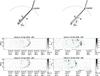 |
Fig. 2 Schematic illustrations of different observation possibilities based on the position of STEREO-A and -B. Left panels illustrate observations when the angular separation ϕ between spacecraft Stereo-A and -B is less than the cone width thickness (α), the radio source illuminates both spacecraft simultaneously. Right panels show observations when angular separation ϕ between spacecraft is larger than α. |
The main idea of the method is based on observations of the same radio burst of the DAM by at least two spacecraft located at different longitudinal separations, as seen from Jupiter, and determination whether both spacecraft are located inside the radio beam or not (see Fig. 2). In particular, the two spacecraft are inside the radio cone wall if their longitudinal Jovicentric separation ϕ is smaller than the angular width of the emission cone wall α (Fig. 2a). Otherwise if ϕ>α they are not located inside the radio cone wall at the moment of observation (Fig. 2b). Therefore, when the two spacecraft are inside the beaming wall, i.e. ϕ<α (Fig. 2a) then the same radio burst is detected nearly simultaneously by both spacecraft. Otherwise, the radio event is detected onboard two spacecraft with a time delay equal to the time which is needed to rotate of the emission cone through the spacecraft separation angle α.
We used the same technique as Kaiser et al. (2000), the pixel-per-pixel cross-correlation. We calculated the 2D cross-correlation between two radio spectra simultaneously recorded by STEREO-A and STEREO-B spacecraft. The correlation results applied to the real observations have to be checked for its statistical significance, since observations always contain some uncertainties due to limited accuracy of an instrument or noise in a system. One method to state statistical significance is to compare the correlation coefficient Cr with its critical value r of the correlation coefficients for a two-tailed test calculated for the given level of significance (in our case 0.05 or 95%) and degree of freedom df = N−2 where N is a number of data points. Only those correlation coefficients which are higher than Cr can be considered as statistically significant. The results are presented as a normalized difference  . Therefore, the cross correlation coefficients Cr are regarded as significant (both spacecraft are inside the emission wall) when Cn> 0. In this case the cross-correlation coefficient Cr is positive and larger than its critical value r. Then we can find the maximal angular spacecraft separation ϕ when Cn> 0 and both spacecraft are illuminated by the same radio source. This angular separation ϕ will define the maximal cone wall thickness of the Jovian DAM.
For the analysis we have selected the data recorded in the decametric frequency range during those time intervals when the angular separation between STEREO-A and STEREO-B as seen from Jupiter was less than 2.5° (Table A.1). The first step of the data analysis was based on visual selection of the proper dynamic spectra. Measured radio events with complex structures, weak signal to noise ratio or when only one spacecraft detected the emission were excluded from the analysis. In total, 139 episodes with arc-like bursts of DAM have been selected.
The number of episodes of Io DAM from the Southern Jovian hemisphere (Io-D and Io-C) was significantly larger than from the Northern hemisphere (Io-A, Io-B). One of the reason was that an occurrence probability of the different components of the DAM emission depends on the declination of the STEREO orbit with respect to the Jovigraphic equatorial plane (Jovicentric declination; Carr et al. 1983). During the years 2007−2009, when most of the episodes with Io-DAM have been observed (see Table A.1) the Jovicentric declination of the STEREO was < 0° and, therefore, mainly Southern sources (Io-D and Io-C) were observed. Additionally, in contrast to the southern sources, the northern ones are observed in broader frequency range. As was shown in Genova & Aubier (1985) and Hess et al. (2011) the maximum radio frequency for the Io-C and Io-D sources is ≈ 25 MHz while for the Io-A and Io-B this frequency can reach ≈ 38 MHz. Since the SWAVES instrument was operated in the frequency range up to 16 MHz it was able to detect only small low frequency part of the Io-A and Io-B arcs. It is also worth noting that the northern sources (Io-A and Io-B) are typically observed as a series of fringe-like broadband patterns most probably due to multiple Alfven wave reflections, e.g. Queinnec & Zarka (1998). These fringe-like spectra were not usable for the calculation of the cross-correlation between dynamic spectra. Therefore, for further analysis we used only Io-C and Io-D arcs to avoid statistical uncertainty due to small numbers of appropriate observations of the Io-A and Io-B DAM (only three events have been clearly recognized in dynamic spectra).
4. Results and conclusion
Figure A.1 shows the normalized correlation coefficients , determined for each event of the DAM, as a function of the angular separation between STEREO/WAVES spacecraft ϕ. The region of spacecraft angular separations ϕ<ϕmin when all the correlation coefficients Cn> 0 and cross-correlation coefficients are statistically significant are indicated in each panel at ϕmin. The ranges of spacecraft angular separations ϕ>ϕmax when all the coefficients Cn< 0 and cross-correlation is not statistically significant is indicated at ϕmax. The region between ϕmin and ϕmaxdenotes a region of ϕ when Cn changes its sign and both positive and negative values of Cn have been obtained.
Figure A.1a shows the Cn for the Io-C DAM. The minimum value of spacecraft separation when all Cn> 0 and both STEREO/WAVES were simultaneously inside the emission cone is ϕmin = 0.9° whereas for ϕ>ϕmax = 1.1° all Cn< 0 and the angular spacecraft separation is larger than emission cone thickness. In the region of ϕ between 0.9°−1.1° the events with Cn> 0 and Cn< 0 have been observed. Therefore, we have evidence that minimum thickness of the Io-C DAM cone wall is 0.9° and the maximum one is 1.1°. The average thickness is 1.0° ± 0.1°. Sharp decrease of the Cn to the values of Cn = −1 at 1.0° of spacecraft angular separation is due to the normalization of the correlation coefficient when Cn = −1 means that Cr is negative (anticorrelation).
Figure A.1b shows the results of determination of the normalized cross-correlation coefficients Cn for the Io-D DAM. Again, we can conclude that the thickness of the Io-D DAM emission cone wall lies between 0.9° and 1.3° and the average thickness is 1.1° ± 0.2°.
The thickness of the non-Io DAM cone wall (Fig. A.1c) is between 1.0°−1.3°. The average value is 1.15° ± 0.15°. In the case of non-Io DAM the coefficients Cn< 0 when the angular separation is larger than 1.3° for most of the
observed spectra except for one point at ϕ = 1.6° (08 Feb., 2012 14:44 UT). A possible explanation of this outlier point is that the emission wall thickness for some of the events can be larger than the averaged one. The other explanation is the presence of the quasi-monochromatic interferences (e.g. man-made radio signals) in the radio observations. Such quasi-monochromatic interferences can introduce false correlation into the dynamic radio spectra simultaneously observed by two spacecraft. We tried to clean DAM observations from such types of the interferences, but the cleaning procedure could not remove all of them. The dynamic spectra non-Io DAM event 08 Feb., 2012 has series of strong interferences between 3 and 3.6 and one intense interference at 7.2 MHz recorded mainly by STEREO-A spacecraft.
As was shown in Fig. A.1, the thickness of Io-C is 1.0° ± 0.1°, 1.1° ± 0.2° for Io-D and 1.15° ± 0.15° for non-Io DAM. The defined thickness are similar within the error range. The averaged width of the emission cone wall for the Io-DAM as well as for the non-Io DAM is about 1.1° ± 0.2°. The obtained results are also in agreement with previous estimations (1.5° ± 0.5°) made by Kaiser et al. (2000) using Wind and Cassini stereoscopic observations.
Acknowledgments
The authors are pleased to acknowledge the Plasma Physics Data Center (CDPP) team for providing the STEREO/WAVES data. This work was financed by the Austrian Science Fund (project P23762-N16). We thank the reviewer for their careful review, constructive comments and valuable suggestions.
References
- Boischot, A., Lecacheux, A., Kaiser, M. L., et al. 1981, J. Geophys. Res., 86, 8213 [NASA ADS] [CrossRef] [Google Scholar]
- Bougeret, J.-L., Kaiser, M. L., Kellogg, P. J., et al. 1995, Space Sci. Rev., 71, 231 [NASA ADS] [CrossRef] [Google Scholar]
- Burke, B. F., & Franklin, K. L. 1955, J. Geophys. Res., 60, 213 [NASA ADS] [CrossRef] [Google Scholar]
- Carr, T. D., Desch, M. D., & Alexander, J. K. 1983, in Physics of the Jovian Magnetosphere, ed. A. J. Dessler (New York: Cambridge Univ. Press), 226 [Google Scholar]
- Genova, F., & Aubier, M. G. 1985, A&A, 150, 139 [NASA ADS] [Google Scholar]
- Goldstein, M. L., & Thieman, J. R. 1981, J. Geophys. Res., 86, 8569 [NASA ADS] [CrossRef] [Google Scholar]
- Hess, S., Cecconi, B., & Zarka, P. 2008, Geophys. Res. Lett., 35, 13107 [NASA ADS] [CrossRef] [Google Scholar]
- Hess, S. L. G., Pétin, A., Zarka, P., Bonfond, B., & Cecconi, B. 2010, Planet. Space Sci., 58, 1188 [NASA ADS] [CrossRef] [Google Scholar]
- Hess, S. L. G., Bonfond, B., Zarka, P., & Grodent, D. 2011, J. Geophys. Res. (Space Physics), 116, 5217 [NASA ADS] [CrossRef] [Google Scholar]
- Kaiser, M. L., Zarka, P., Kurth, W. S., Hospodarsky, G. B., & Gurnett, D. A. 2000, J. Geophys. Res., 105, 16053 [NASA ADS] [CrossRef] [MathSciNet] [Google Scholar]
- Lecacheux, A., Boudjada, M. Y., Rucker, H. O., et al. 1998, A&A, 329, 776 [NASA ADS] [Google Scholar]
- Queinnec, J., & Zarka, P. 1998, J. Geophys. Res., 103, 26649 [NASA ADS] [CrossRef] [Google Scholar]
- Ray, L. C., & Hess, S. 2008, J. Geophys. Res. (Space Physics), 113, 11218 [Google Scholar]
- Treumann, R. A. 2006, A&ARv, 13, 229 [NASA ADS] [CrossRef] [Google Scholar]
- Wu, C. S., & Lee, L. C. 1979, ApJ, 230, 621 [NASA ADS] [CrossRef] [Google Scholar]
- Zarka, P. 1998, J. Geophys. Res., 103, 20159 [NASA ADS] [CrossRef] [Google Scholar]
- Zarka, P., Le Queau, D., & Genova, F. 1986, J. Geophys. Res., 91, 13542 [NASA ADS] [CrossRef] [Google Scholar]
- Zarka, P., Ryabov, B. P., Ryabov, V. B., et al. 1997, On the Origin of Jovian Decameter Radio Bursts, eds. H. O. Rucker, S. J. Bauer, & A. Lecacheux, 51 [Google Scholar]
Appendix A: Additional data
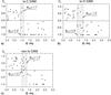 |
Fig. A.1 Normalized correlation coefficients |
Periods of time in the years 2007−2014 when the angular separation between STEREO-A and STEREO-B was less than 2.5°.
All Tables
Periods of time in the years 2007−2014 when the angular separation between STEREO-A and STEREO-B was less than 2.5°.
All Figures
|
Fig. 1 Identification of the radio emission observed stereoscopically by STEREO/WAVES. Panel a) shows the solar type III radio burst observed simultaneously (dt ≈ 0) by STEREO-A (STA) and STEREO-B (STB). Panels b) and c) display examples of the DAM emission. The radiation on panel b) was observed sequentially by both spacecraft with time delay (dt ≈ 0.71 h) which corresponds to ≈ 26° of Jupiter’s rotation and ≈ 6.0° of the Io angular shift along its orbit. Since the angular separation between both spacecraft as seen from Jupiter was ≈ 6.3° we conclude that the observed radio emission is Io related DAM (see Sect. 2). Panel c) illustrates the identification of non-Io DAM. The spectra in b) and c) are plotted with a correction for difference in light travel time from Jupiter to each of the spacecraft. |
| In the text | |
|
Fig. 2 Schematic illustrations of different observation possibilities based on the position of STEREO-A and -B. Left panels illustrate observations when the angular separation ϕ between spacecraft Stereo-A and -B is less than the cone width thickness (α), the radio source illuminates both spacecraft simultaneously. Right panels show observations when angular separation ϕ between spacecraft is larger than α. |
| In the text | |
|
Fig. A.1 Normalized correlation coefficients |
| In the text | |
Current usage metrics show cumulative count of Article Views (full-text article views including HTML views, PDF and ePub downloads, according to the available data) and Abstracts Views on Vision4Press platform.
Data correspond to usage on the plateform after 2015. The current usage metrics is available 48-96 hours after online publication and is updated daily on week days.
Initial download of the metrics may take a while.