| Issue |
A&A
Volume 594, October 2016
|
|
|---|---|---|
| Article Number | A75 | |
| Number of page(s) | 4 | |
| Section | Stellar atmospheres | |
| DOI | https://doi.org/10.1051/0004-6361/201629222 | |
| Published online | 13 October 2016 | |
The nature of the light variability of magnetic Of?p star HD 191612
Ústav teoretické fyziky a astrofyziky, Masarykova univerzita, Kotlářská 2, 611 37 Brno, Czech Republic
e-mail: This email address is being protected from spambots. You need JavaScript enabled to view it.
Received: 30 June 2016
Accepted: 16 August 2016
Abstract
Context. A small fraction of hot OBA stars host global magnetic fields with field strengths of the order of 0.1−10 kG. This leads to the creation of persistent surface structures (spots) in stars with sufficiently weak winds as a result of the radiative diffusion. These spots become evident in spectroscopic and photometric variability. This type of variability is not expected in stars with strong winds, where the wind inhibits the radiative diffusion. Therefore, a weak photometric variability of the magnetic Of?p star HD 191612 is attributed to the light absorption in the circumstellar clouds.
Aims. We study the nature of the photometric variability of HD 191612. We assume that the variability results from variable wind blanketing induced by surface variations of the magnetic field tilt and modulated by stellar rotation.
Methods. We used our global kinetic equilibrium (NLTE) wind models with radiative force determined from the radiative transfer equation in the comoving frame (CMF) to predict the stellar emergent flux. Our models describe the stellar atmosphere in a unified manner and account for the influence of the wind on the atmosphere. The models are calculated for different wind mass-loss rates to mimic the effect of magnetic field tilt on the emergent fluxes. We integrate the emergent fluxes over the visible stellar surface for individual rotational phases, and calculate the rotationally modulated light curve of HD 191612.
Results. The wind blanketing that varies across surface of HD 191612 is able to explain a part of the observed light variability in this star. The mechanism is able to operate even at relatively low mass-loss rates. The remaining variability is most likely caused by the flux absorption in circumstellar clouds.
Conclusions. The variable wind blanketing is an additional source of the light variability in massive stars. The presence of the rotational light variability may serve as a proxy for the magnetic field.
Key words: stars: winds, outflows / stars: mass-loss / stars: early-type / stars: variables: general / hydrodynamics
© ESO, 2016
1. Introduction
A small fraction of hot OBA stars host global magnetic fields with surface intensities of the order of 0.1−10 kG (Romanyuk 2014; Wade et al. 2016). This leads to the creation of persistent surface structures (spots) in stars with low luminosity (weak or absent winds) as a result of the radiative diffusion (Vauclair 1975; Vick et al. 2011). These spots cause prominent spectroscopic variability, which is modulated by the stellar rotation (e.g. Lüftinger et al. 2010; Kochukhov et al. 2014). The inhomogeneous surface distribution of elements and redistribution of the flux in the surface spots leads to the photometric variability of chemically peculiar stars (Krtička et al. 2015; Prvák et al. 2015).
This type of variability is not expected in magnetic stars with strong winds, where the wind is predicted to inhibit the radiative diffusion (Vauclair 1975; Vick et al. 2011). Instead, the magnetic field interacts with the ionized stellar wind, which moves along the field lines. The effect of the magnetic field on the stellar wind is characterized by the ratio between magnetic field energy density and kinetic energy density of the wind. This may be parameterized by the wind magnetic confinement parameter introduced by ud-Doula & Owocki (2002). The larger the magnetic field energy density is, the stronger is the influence of the magnetic field on the flow. If the magnetic field energy density dominates, then the structure of the flow depends on the relation between the Kepler corotation radius RK, at which the centrifugal force balances the gravity, and the Alfvén radius RA (see ud-Doula et al. 2008; Petit et al. 2013), where the flow velocity is equal to the Alfvén speed. The magnetosphere displays dynamical phenomena for slowly rotating stars with RA<RK, whereas circumstellar clouds exist in stars hosting centrifugal magnetospheres with RA>RK.
Therefore, observed weak photometric variability of the magnetic Of?p star HD 191612 was attributed to the light absorption in the circumstellar clouds rather than to surface spots (Wade et al. 2011). However, we argue that photometric spots may exist even on the surface of hot stars with magnetic fields and winds. These are not caused by the abundance inhomogeneities, but by wind mass flux that is modulated by the different tilt of the magnetic field across the stellar surface.
As the wind is forced to flow along the magnetic field in the strong field limit, only a projection of the radiative force along the field lines is able to accelerate the wind. Therefore, the surface wind mass flux depends on the magnetic field tilt with respect to the surface normal and therefore on the location on the stellar surface (Owocki & ud-Doula 2004). The wind blocks part of the photospheric flux affecting the emergent flux and photometric colours (Abbott & Hummer 1985). This effect is called wind blanketing and has to be modelled by a global atmosphere models that unify the description of the photosphere and wind (Hillier & Miller 1998; Gräfener et al. 2002; Puls et al. 2005). Such models take the feedback effect of the stellar wind on the photosphere properly into the account.
To our knowledge, the wind blanketing has never been studied as a source of the light variability in magnetic O stars. For this purpose we selected Of?p star HD 191612. This star has a relatively strong stellar wind (Marcolino et al. 2013). The period of weak photometric variability of this star of 536 days (Koen & Eyer 2002; Nazé 2004) is consistent with the period of spectral variability (Walborn et al. 2004). The discovery of a strong magnetic field with a polar strength of about − 1.5 kG (Donati et al. 2006) led to the current picture of rotationally modulated variability of this star, which aims to explain the optical and ultraviolet (UV) line variability (Sundqvist et al. 2012; Marcolino et al. 2013), longitudinal magnetic field variability (Wade et al. 2011), and the variability of X-ray flux (Nazé et al. 2010).
The photometric variability of HD 191612 was successfully modelled with the Monte Carlo radiative transfer code, which used the density structure from the magnetohydrodynamic simulations (Wade et al. 2011). The simulations adopted a relatively high wind mass-loss rate 1.6 × 10⁻⁶M⊙ yr-1, which was derived by Howarth et al. (2007) from Hα spectroscopy. However, the mass-loss rate derived from the UV diagnostics 1.3 × 10⁻⁸M⊙ yr-1 (Marcolino et al. 2013) is more than two orders of magnitude lower. This difference likely reflects the problem of discordant mass-loss rate determinations in O stars that is attributed to clumping (e.g. Puls et al. 2006; Sundqvist et al. 2011; Šurlan et al. 2012, 2013). Anyway, it would likely be problematic to explain the observed light variability with such a low wind mass-loss rate. Therefore, we study the wind blanketing as a potential additional source of the light variability in HD 191612.
2. Global wind models
We used our spherically symmetric stationary wind code METUJE (Krtička & Kubát, in prep.) for the calculation of the wind models of HD 191612. The code is based on our previous models (Krtička & Kubát 2010), however it is calculated in a global (unified) approach that integrates the description of the hydrostatic atmosphere and supersonic wind. The model radiative transfer equation is solved in the comoving frame (CMF) with opacities and emissivities calculated using occupation numbers that are derived from the kinetic equilibrium (NLTE) equations. For given stellar parameters, the model enables us to predict consistently the radial wind structure (i.e. the radial dependence of density, velocity, and temperature) from hydrodynamical equations and to derive the wind mass-loss rate Ṁ and the stellar emergent flux that accounts for the wind blanketing.
The ionization and excitation state was calculated from the NLTE equations. Part of the corresponding models of ions (see Krtička & Kubát 2009, for a complete list) was adopted from TLUSTY model atmosphere input files (Lanz & Hubeny 2003, 2007) and part was prepared by us using Opacity and Iron Project data (Seaton et al. 1992; Hummer et al. 1993) and data described by Pauldrach et al. (2001). The level populations were used to calculate opacities and emissivities in the CMF radiative transfer equation. The radiative transfer equation was solved with a method of Mihalas et al. (1975) modified by Krtička & Kubát (2010). We used the diffusion approximation as the inner boundary condition. The solution of the radiative transfer equation was used to calculate the radiative rates in the NLTE equations, the radiative force, and the radiative cooling and heating terms. For the determination of the temperature we used three different methods depending on the location in the atmosphere and wind. In the deepest layers of the atmosphere we used the differential form of the radiative equilibrium, while in the upper layers of the atmosphere we applied the integral form of the radiative equilibrium (e.g. Kubát 1996); in the wind we used the thermal balance on free electrons method (Kubát et al. 1999). The hydrodynamical equations (the continuity equation, equation of motion, and the energy equation) were solved iteratively together with NLTE and radiative transfer equations to obtain the radial dependence of level populations, density, radial velocity, and temperature. The line data used for the line force calculation were extracted from the VALD database (Piskunov et al. 1995, Kupka et al. 1999) supplemented for lighter elements (with atomic number Z ≤ 20) using the data available at the Kurucz website1. The initial model for the iterations was derived from the combination of the model atmosphere calculated with TLUSTY (Lanz & Hubeny 2003) in the inner parts of the global model and in the outer parts of the wind model.
For our study we adopted the HD 191612 parameters given in Table 1. The effective temperature taken from Marcolino et al. (2013) was used to derive mass and radius from scalings of Martins et al. (2005). The adopted radius agrees with that derived by Howarth et al. (2007) and Marcolino et al. (2013) and the mass agrees with the estimate of Howarth et al. (2007). The mass-loss rate was predicted by our METUJE models neglecting the effect of the magnetic field. Our predicted value is intermediate between the values derived from the optical and UV analysis (Howarth et al. 2007; Marcolino et al. 2013). We assumed solar chemical composition (Asplund et al. 2009).
Our wind modelling neglects the influence of the magnetic field. In reality the wind flows along the magnetic field lines, which affects its dynamics as a result of the tilt of the flow with respect to the radial direction and modified divergence of the flow (ud-Doula & Owocki 2002). However, we are concerned with the influence of magnetic field on the wind blanketing, which is governed mostly by the wind mass-loss rate. To model this effect, we artificially scale the radiative force in the wind. This yields a series of wind models and emergent fluxes F(λ,Ṁ) parameterized by the wind mass-loss rate.
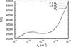 |
Fig. 1 Dependence of the wind temperature as a function of the electron density for models with different mass-loss rates. |
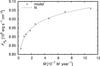 |
Fig. 2 Dependence of the emergent flux in the Hp colour of the Hipparcos photometric system on the wind mass-loss rate. Crosses denote the values from the models and the dashed line fit Eq. (2). |
The wind blanketing increases with increasing wind mass-loss rate. This results in the increase of the temperature of the continuum forming region of the model atmosphere (see Fig. 1) and causes the modification of the emergent flux in the individual photometric passbands. Therefore, the Hp flux of the Hipparcos photometric system FHp(Ṁ) depends on the wind mass-loss rate, as shown in Fig. 2. The emergent flux in passband Hp for a given mass-loss rate was calculated as 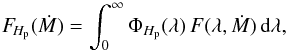 (1)where ΦHp(λ) is the response function of the Hipparcos photometric system. Fitting the emergent fluxes for different mass-loss rates we arrive at approximate formula
 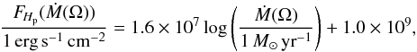 (2)which gives an emergent flux in passband Hp as a function of mass-loss rate. Because we fitted the flux variations with a power law, the resulting light curve is expected to be independent of an exact value of the mass-loss rate. This shows that the studied mechanism can cause the light variability even at a relatively low mass-loss rates.
3. Modelling of the light variability of HD 191612
We modified our code for the prediction of the light variability of chemically peculiar stars (Krtička et al. 2015) to model the light variability due to the wind blanketing. The magnitude difference between the flux fHp at a given phase and the reference flux  in passband Hp is defined as
  (3)The reference flux is obtained under the condition that the mean magnitude difference over the rotational period is zero. The radiative flux in a passband Hp at the distance D from the spherical star is (Hubeny & Mihalas 2014)
  (4)The intensity IHp(θ,Ω) at angle θ with respect to the normal at the surface was obtained at each surface point with spherical coordinates Ω from the emergent flux taking into account the limb darkening uHp(θ)
 (5)with limb darkening coefficients from Reeve & Howarth (2016). Here
  . The emergent flux FHp(Ṁ(Ω)) as a function of mass-loss rate is taken from the fit Eq. (2). The mass-loss rate was assumed to depend on the tilt of the magnetic field as (Owocki & ud-Doula 2004)
 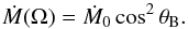 (6)This scaling was derived from analytical considerations, but it agrees with numerical simulations. The mass-loss rate Ṁ0, which neglects the influence of the magnetic field is given in Table 1.
For a dipolar magnetic field 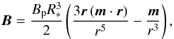 (7)where Bp is the polar magnetic field strength, r is the radius vector, and m is the unit vector in the direction of the magnetic pole, the tilt of the magnetic field is given by a scalar product
 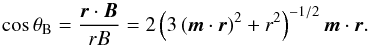 (8)In the models, the tilt of the magnetic field θB was derived assuming the dipolar field inclined by angle β with respect to the rotational axis. The axis of rotation is inclined by angle i with respect to the line of sight.
There is no unique measurement of the rotational axis inclination i and magnetic field obliquity β, however, the observations yield the sum of these two values i + β = 95° (Wade et al. 2011). Taking advantage of this liberty, we selected parameters that fit the observed data best, i.e. i = 50° and β = 45°. The light curves with other parameters have similar shapes but lower amplitudes.
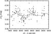 |
Fig. 3 Comparison of simulated (solid line) and observed (Hipparcos, dots) light curve of HD 191612. The light curve was plotted using the ephemeris of Howarth et al. (2007). |
The observed and simulated light curves show the light maximum during the phases when the magnetic pole is visible on the stellar surface (Fig. 3). The stellar wind flows freely along the magnetic field lines during these phases, and consequently the mass-loss rate and the visual magnitude are the highest. On the other hand, during the light minimum the magnetic equator appears on the visible surface, and consequently the mass-loss rate is inhibited and the visual flux is the lowest.
The observed and predicted light curves agree in shape. However, the observed light curve has amplitude 35 ± 4 mmag, which is about three times higher than the amplitude of the predicted light curve. Consequently, our model is able to explain at most part of the light variability of HD 191612.
4. Conclusions and discussion
We modelled the light variability of HD 191612 assuming that the light variability is caused by the influence of magnetic field on the wind mass flux. The tilt of the magnetic field varies across the HD 191612 surface, and consequently the wind mass flux depends on the location on the stellar surface. As a result of the wind blanketing, which increases with mass-loss rate, the emergent flux is redistributed partly to the optical region. The stellar rotation modulates the observed flux and leads to light variability.
The observed and predicted light curves agree in shape, but the observed light curve has about three times higher amplitude than the predicted light curve. The missing light variability can be explained by light absorption in the circumstellar clouds (Wade et al. 2011).
The proposed mechanism is able to operate even at moderate mass-loss rates, which are significantly lower than that inferred from the Hα analysis. The importance of the wind blanketing for light variability can be observationally tested in the UV domain. Our calculations showed that light variability in the UV (e.g. around 1300 Å) is in the anti-phase with visual variability.
The influence of the Zeeman effect on the opacity may also contribute to light variability in magnetic stars. However, the detailed model atmosphere calculations with anomalous Zeeman effect and polarized radiative transfer (Khan & Shulyak 2006) performed for A stars showed that such an effect is important only in stars with much stronger fields. The influence of this effect in HD 191612 is therefore likely to be negligible.
The atmosphere of magnetic stars has a 3D structure and cannot be modelled with spherically symmetric models in general. However, the most important effect due to the magnetic field, i.e. the influence on the wind mass-loss rate, was included in the models. The emergent flux is not significantly influenced by the 3D effects, because the continuum forming region has significantly smaller thickness than a typical scale at which the magnetic field varies.
The study of the magnetic fields is especially important in O stars. Similar to the chemically peculiar stars, light variability may serve as a proxy for the search of the magnetic field using spectropolarimetry. The origin of the magnetic field is still a matter of the debate. The magnetic fields dominates the atmospheres of stars with a magnetic field of the order of 100 G and stronger, but the magnetic field energy density is lower than the gas thermal energy density inside the stars. Consequently, it is likely that the interstellar magnetic field does not survive the initial violent period of star formation and the surface magnetic field is most likely the descendant of the dynamo magnetic field from the period of star formation (Braithwaite 2008).
Magnetic A stars do not have strong winds, and consequently in these stars we always observe the same layers during the main-sequence lifetime. However, in O stars the material from the stellar atmosphere is blown away by strong winds within days, and hence we always observe freshly exposed layers of the stars. The detection of the magnetic field therefore shows that the magnetic fields threads the deep subsurface layers of these stars. Moreover, the study of time variability of this field (even just from the photometric variations) can provide information about the magnetic field variation inside the stars.
Acknowledgments
This research was supported by grant GA ČR 16-01116S. Access to computing and storage facilities owned by parties and projects contributing to the National Grid Infrastructure MetaCentrum, provided under the programme Projects of Large Infrastructure for Research, Development, and Innovations (LM2010005), is greatly appreciated.
References
- Abbott, D. C., & Hummer, D. G. 1985, ApJ, 294, 286 [NASA ADS] [CrossRef] [Google Scholar]
- Asplund, M., Grevesse, N., Sauval, A. J., & Scott, P. 2009, ARA&A, 47, 481 [NASA ADS] [CrossRef] [Google Scholar]
- Braithwaite, J. 2008, MNRAS, 386, 1947 [NASA ADS] [CrossRef] [Google Scholar]
- Donati, J.-F., Howarth, I. D., Bouret, J.-C., et al. 2006, MNRAS, 365, L6 [NASA ADS] [CrossRef] [Google Scholar]
- Gräfener, G., Koesterke, L., & Hamann, W.-R. 2002, A&A, 387, 244 [NASA ADS] [CrossRef] [EDP Sciences] [Google Scholar]
- Hillier, D. J., & Miller, D. L. 1998, ApJ, 496, 407 [NASA ADS] [CrossRef] [Google Scholar]
- Howarth, I. D., Walborn, N. R., Lennon, D. J., et al. 2007, MNRAS, 381, 433 [NASA ADS] [CrossRef] [Google Scholar]
- Hubeny, I., & Mihalas, D., 2014, Theory of Stellar Atmospheres (Princeton: Princeton University Press) [Google Scholar]
- Hummer, D. G., Berrington, K. A., Eissner, W., et al. 1993, A&A, 279, 298 [NASA ADS] [Google Scholar]
- Khan, S. A., & Shulyak, D. 2006, A&A, 448, 113 [Google Scholar]
- Kochukhov, O., Lüftinger, T., Neiner, C., Alecian, E., & MiMeS Collaboration 2014, A&A, 565, A83 [NASA ADS] [CrossRef] [EDP Sciences] [Google Scholar]
- Koen, C., & Eyer, L. 2002, MNRAS, 331, 45 [NASA ADS] [CrossRef] [Google Scholar]
- Krtička, J., & Kubát, J. 2009, MNRAS, 394, 2065 [NASA ADS] [CrossRef] [Google Scholar]
- Krtička, J., & Kubát, J. 2010, A&A, 519, A5 [NASA ADS] [CrossRef] [EDP Sciences] [Google Scholar]
- Krtička, J., Mikulášek, Z., Lüftinger, T., & Jagelka, M. 2015, A&A, 576, A82 [NASA ADS] [CrossRef] [EDP Sciences] [Google Scholar]
- Kubát, J. 1996, A&A, 305, 255 [NASA ADS] [Google Scholar]
- Kubát, J., Puls, J., & Pauldrach, A. W. A. 1999, A&A, 341, 587 [NASA ADS] [Google Scholar]
- Kupka, F., Piskunov, N. E., Ryabchikova, T. A., Stempels, H. C., & Weiss, W. W. 1999, A&AS, 138, 119 [NASA ADS] [CrossRef] [EDP Sciences] [MathSciNet] [PubMed] [Google Scholar]
- Lanz, T., & Hubeny, I. 2003, ApJS, 146, 417 [NASA ADS] [CrossRef] [Google Scholar]
- Lanz, T., & Hubeny, I. 2007, ApJS, 169, 83 [CrossRef] [Google Scholar]
- Lüftinger, T., Kochukhov, O., Ryabchikova, T., et al. 2010, A&A, 509, A71 [NASA ADS] [CrossRef] [EDP Sciences] [Google Scholar]
- Marcolino, W. L. F., Bouret, J.-C., Sundqvist, J. O., et al. 2013, MNRAS, 431, 2253 [NASA ADS] [CrossRef] [Google Scholar]
- Martins, F., Schaerer, D., & Hillier, D. J. 2005, A&A, 436, 1049 [NASA ADS] [CrossRef] [EDP Sciences] [Google Scholar]
- Mihalas, D., Kunasz, P. B., & Hummer, D. G. 1975, ApJ, 202, 465 [NASA ADS] [CrossRef] [Google Scholar]
- Nazé, Y. 2004, Ph.D. Thesis, Univ. Liège [Google Scholar]
- Nazé, Y., Ud-Doula, A., Spano, M., et al. 2010, A&A, 520, A59 [NASA ADS] [CrossRef] [EDP Sciences] [Google Scholar]
- Owocki, S. P., & ud-Doula, A. 2004, ApJ, 600, 1004 [NASA ADS] [CrossRef] [Google Scholar]
- Pauldrach, A. W. A., Hoffmann, T. L., & Lennon, M. 2001, A&A, 375, 161 [NASA ADS] [CrossRef] [EDP Sciences] [Google Scholar]
- Petit, V., Owocki, S. P., Wade, G. A., et al. 2013, MNRAS, 429, 398 [NASA ADS] [CrossRef] [Google Scholar]
- Piskunov, N. E., Kupka, F., Ryabchikova, T. A., Weiss, W. W., & Jeffery, C. S. 1995, A&AS, 112, 525 [NASA ADS] [Google Scholar]
- Prvák, M., Liška, J., Krtička, J., Mikulášek, Z., & Lüftinger, T. 2015, A&A, 584, A17 [NASA ADS] [CrossRef] [EDP Sciences] [Google Scholar]
- Puls, J., Urbaneja, M. A., Venero, R., et al. 2005, A&A, 435, 669 [NASA ADS] [CrossRef] [EDP Sciences] [Google Scholar]
- Puls, J., Markova, N., Scuderi, S., et al. 2006, A&A, 454, 62 [Google Scholar]
- Reeve, D. C., & Howarth, I. D. 2016, MNRAS, 456, 1294 [NASA ADS] [CrossRef] [Google Scholar]
- Romanyuk, I. I. 2014, Putting A Stars into Context: Evolution, Environment, and Related Stars, 371 [Google Scholar]
- Seaton, M. J., Zeippen, C. J., Tully, J. A., et al. 1992, Rev. Mex. Astron. Astrofis., 23, 19 [NASA ADS] [EDP Sciences] [Google Scholar]
- Sundqvist, J. O., Puls, J., Feldmeier, A., & Owocki, S. P. 2011, A&A, 528, A6 [Google Scholar]
- Sundqvist, J. O., ud-Doula, A., Owocki, S. P., et al. 2012, MNRAS, 423, L21 [NASA ADS] [CrossRef] [Google Scholar]
- Šurlan, B., Hamann, W.-R., Kubát, J., Oskinova, L., & Feldmeier, A. 2012, A&A, 541, A37 [NASA ADS] [CrossRef] [EDP Sciences] [Google Scholar]
- Šurlan, B., Hamann, W.-R., Aret, A., et al. 2013, A&A, 559, A130 [NASA ADS] [CrossRef] [EDP Sciences] [Google Scholar]
- ud-Doula, A., & Owocki, S. P. 2002, ApJ, 576, 413 [NASA ADS] [CrossRef] [Google Scholar]
- ud-Doula, A., Owocki, S. P., & Townsend, R. H. D. 2008, MNRAS, 385, 97 [NASA ADS] [CrossRef] [Google Scholar]
- Vauclair, S. 1975, A&A, 45, 233 [NASA ADS] [Google Scholar]
- Vick, M., Michaud, G., Richer, J., & Richard, O. 2011, A&A, 526, A37 [NASA ADS] [CrossRef] [EDP Sciences] [Google Scholar]
- Wade, G. A., Howarth, I. D., Townsend, R. H. D., et al. 2011, MNRAS, 416, 3160 [NASA ADS] [CrossRef] [Google Scholar]
- Wade, G. A., Neiner, C., Alecian, E., et al. 2016, MNRAS, 456, 2 [NASA ADS] [CrossRef] [Google Scholar]
- Walborn, N. R., Howarth, I. D., Rauw, G., et al. 2004, ApJ, 617, L61 [NASA ADS] [CrossRef] [Google Scholar]
All Tables
All Figures
|
Fig. 1 Dependence of the wind temperature as a function of the electron density for models with different mass-loss rates. |
| In the text | |
|
Fig. 2 Dependence of the emergent flux in the Hp colour of the Hipparcos photometric system on the wind mass-loss rate. Crosses denote the values from the models and the dashed line fit Eq. (2). |
| In the text | |
|
Fig. 3 Comparison of simulated (solid line) and observed (Hipparcos, dots) light curve of HD 191612. The light curve was plotted using the ephemeris of Howarth et al. (2007). |
| In the text | |
Current usage metrics show cumulative count of Article Views (full-text article views including HTML views, PDF and ePub downloads, according to the available data) and Abstracts Views on Vision4Press platform.
Data correspond to usage on the plateform after 2015. The current usage metrics is available 48-96 hours after online publication and is updated daily on week days.
Initial download of the metrics may take a while.