| Issue |
A&A
Volume 594, October 2016
|
|
|---|---|---|
| Article Number | A111 | |
| Number of page(s) | 16 | |
| Section | Numerical methods and codes | |
| DOI | https://doi.org/10.1051/0004-6361/201628220 | |
| Published online | 20 October 2016 | |
Analysis of the Bayesian Cramér-Rao lower bound in astrometry
Studying the impact of prior information in the location of an object
1 Information and Decision Systems Group, Department of Electrical Engineering, Universidad de Chile, Av. Tupper 2007, Santiago, Chile
e-mail:
aecheverria@ing.uchile.cl
2 Departamento de Astronomía, Facultad de Ciencias Físicas y Matemáticas, Universidad de Chile, Casilla 36-D, Santiago, Chile
e-mail:
rmendez@uchile.cl
Received: 29 January 2016
Accepted: 9 July 2016
Context. The best precision that can be achieved to estimate the location of a stellar-like object is a topic of permanent interest in the astrometric community.
Aims. We analyze bounds for the best position estimation of a stellar-like object on a CCD detector array in a Bayesian setting where the position is unknown, but where we have access to a prior distribution. In contrast to a parametric setting where we estimate a parameter from observations, the Bayesian approach estimates a random object (i.e., the position is a random variable) from observations that are statistically dependent on the position.
Methods. We characterize the Bayesian Cramér-Rao (CR) that bounds the minimum mean square error (MMSE) of the best estimator of the position of a point source on a linear CCD-like detector, as a function of the properties of detector, the source, and the background.
Results. We quantify and analyze the increase in astrometric performance from the use of a prior distribution of the object position, which is not available in the classical parametric setting. This gain is shown to be significant for various observational regimes, in particular in the case of faint objects or when the observations are taken under poor conditions. Furthermore, we present numerical evidence that the MMSE estimator of this problem tightly achieves the Bayesian CR bound. This is a remarkable result, demonstrating that all the performance gains presented in our analysis can be achieved with the MMSE estimator.
Conclusions. The Bayesian CR bound can be used as a benchmark indicator of the expected maximum positional precision of a set of astrometric measurements in which prior information can be incorporated. This bound can be achieved through the conditional mean estimator, in contrast to the parametric case where no unbiased estimator precisely reaches the CR bound.
Key words: astrometry / methods: statistical / methods: analytical / instrumentation: detectors / methods: data analysis
© ESO, 2016
1. Introduction
Astrometry, which relies on the precise determination of the relative location of point sources, is the foundation of classical astronomy and modern astrophysics, and it will remain a cornerstone of the field for the 21st century. Historically, it was the first step in the evolution of astronomy from phenomenology to a science that is rooted in precise measurements and physical theory. Astrometry spans more than two thousand years, from Hipparchus (ca. 130 BC) and Ptolemy (150 AD) to modern digital-based all sky surveys, from the ground and in space. The dramatic improvement in accuracy reflects this historic time scale (Høg 2011, see, e.g., his Fig. 4). Nowadays, astronomers take for granted resources such as the ESA Hipparcos mission, which yielded a catalog of more than 100 000 stellar positions to an accuracy of 1 milliarcsecond, and look forward to the results of the ESA Gaia astrometric satellite, which will deliver a catalog of over 109 stars with accuracies smaller than 10–20 mas for objects brighter than V = 15 and a completeness limit of V = 20.
The determination of the best precision that can be achieved to determine the location of a stellar-like object has been a topic of permanent interest in the astrometric community (van Altena & Auer 1975; Lindegren 1978; Auer & Van Altena 1978; Lee & van Altena 1983; Winick 1986; Jakobsen et al. 1992; Adorf 1996; Bastian 2004; Lindegren 2010). One of the tools used to characterize this precision is the Cramér-Rao (CR) bound, which provides a lower bound for the variance that can be achieved to estimate (with an unbiased estimator) the position of a point source (Mendez et al. 2013, 2014; Lobos et al. 2015), given the properties of the source and the detector. In astrometry this CR bound offers meaningful closed-form expressions that can be used to analyze the complexity of the inference task in terms of key observational and design parameters, such as position of the object in the array, pixel resolution of the instrument, and background. In particular, Mendez et al. (2013, 2014) have developed closed-form expressions for this bound and have studied its structure and dependency with respect to important observational parameters. Furthermore, the analysis of the CR bound allows us to address the problem of optimal pixel resolution of the array for a given observational setting, and in general to evaluate the complexity of the astrometric task with respect to the signal-to-noise ratio (S/N) and different observational regimes. Complementing these results, Lobos et al. (2015) have studied the conditions under which the CR bound can be achieved by a practical estimator. In that context, the least-squares estimator has been analyzed to show the regimes where this scheme is optimal with respect to the CR bound. On the other hand, Bouquillon et al. (2016) have applied the CR bound to moving sources and compared the CR predictions to observations of the Gaia satellite with the VLT Survey Telescope at ESO, showing very good correspondence between the expectations and the measured positional uncertainties.
In this work we extend the astrometric analysis mentioned above, transiting from the classical parametric setting, where the position is considered fixed but unknown, to the richer Bayesian setting, where the position is unknown but the prior distribution of the object position is available. This changes in a fundamental way the nature of the inference problem from a parametric context in which we are estimating a constant parameter from a set of random observations to a random setting in which we estimate a random object (i.e., the position is modeled as a random variable) from observations that are statistically dependent with the position.
The use of a Bayesian approach to astrometry is not new; we note, for example, that recently (Michalik et al. 2015b) and (Michalik & Lindegren 2016) have proposed analyzing part of the data from the Gaia astrometric satellite using a suitable chosen set of priors in a Bayesian context. In Michalik et al. (2015b), the feasibility of the Bayesian approach, especially for the analysis of stars with poor observation histories, is demonstrated through global astrometric solutions of simulated Gaia observations. In this case, the prior information is derived from reasonable assumptions regarding the distributions of proper motions and parallaxes. On the other hand, in (Michalik & Lindegren 2016) they show how the prior information regarding QSO proper motions could provide an independent verification of the parallax zero-point for the early reduction of Gaia data in the context of the HTPM project, which uses Hipparcos stars as first epoch (Mignard 2009; Michalik et al. 2014), or the TGAS project, which uses the Tycho-2 stars as first epoch (Michalik et al. 2015a).
An important new element of the Bayesian setting is the introduction of a prior distribution of the object position. Therefore, the conceptual question to address is to quantify and analyze the increase in astrometric performance from the use of a prior distribution of the object position, information that is not available (or used) in the classical parametric setting. To the best of our knowledge, this direction has not been addressed systematically by the community and remains an interesting open problem. In this work, we tackle this problem from a theoretical and numerical point of view, and we provide some concrete practical implications.
On the theoretical side, we consider the counterpart of the CR bound in the Bayesian context, which is known as the Van Trees’ inequality, or Bayesian CR bound (Van Trees 2004). As was the case in the parametric scenario, the Bayesian CR bound offers a tight performance bound, more precisely a lower bound for the minimum mean square error (MSE) of the best estimator for the position in the Bayes setting. The first part of this work is devoted to formalize the Bayesian problem of astrometry and to develop closed-form expressions for the Bayesian CR as well as an expression to estimate the gain in performance. As in the parametric case, different observational regimes are evaluated to quantify the gain induced from the prior distribution of the object location. On this, we introduce formal definitions for the prior information and the information attributed to the observations, and with these concepts the notion of when the information of the prior distribution is relevant or irrelevant with respect to the information provided by the observations. This last distinction determines when there is a significant gain in astrometric precision from the prior distribution. A powerful corollary of this analysis is that the Bayes setting always offers a better performance than the parametric setting, even in the worse-case prior (i.e., that of a uniform distribution).
On the practical side, we consider some realistic experimental conditions to evaluate numerically the gain of the Bayes setting with respect to the parametric scenario. Remarkably, it is shown that the gain in performance is significant for various observational regimes in astrometry, which is particularly clear in the case of faint objects, or when the observations are acquired under poor conditions (i.e., in the low S/N regime). An alternative concrete way to illustrate this gain in performance is elaborated in Sect. 6, where we introduce the concept of the equivalent object brightness. On the estimation side, we submit evidence that the minimum mean square error (MMSE) estimator of this problem (the well-known conditional mean estimator) tightly achieves the Bayesian CR lower bound. This is a remarkable result, demonstrating that all the performance gains presented in the theoretical analysis part of our paper can indeed be achieved with the MMSE estimator, which in principle has a practical implementation (Weinstein & Weiss 1988). We end our paper with a simple example of what could be achieved using the Bayesian approach in terms of the astrometric precision when new observations of varying quality are used and we incorporate as prior information data from the USNO-B all-sky catalog.
2. Preliminaries
In this section we introduce the problem of astrometry as well as the concepts and definitions that will be used throughout the paper. For simplicity, we focus on the 1D scenario of a linear array detector, as it captures the key conceptual elements of the problem1.
2.1. Astrometry
The problem we want to tackle is the inference of the position of a point source with respect to the (known) relative location of the picture elements of a detector array. This source is parameterized by three scalar quantities, the angular position in the sky (measured in seconds of arc [arcsec]) of the object xc ∈R in the array, its intensity (or brightness, or flux) that we denote by  , and a generic parameter that determines the width (or spread) of the light distribution on the detector, denoted by σ ∈ R+. These parameters induce a probability over an observation space that we denote by X. More precisely, given a point source represented by the triad
  , it creates a nominal intensity profile in a photon integrating device (PID), typically a CCD, which can be generally written as:
  (1)where φ(x − xc,σ) denotes the 1D normalized point spread function (PSF). In what follows,
  and σ are assumed to be known and fixed, and consequently they are not part of the inference problem addressed here.
In practice, the PSF described by Eq. (1) cannot be observed with infinite precision, mainly because of three disturbances (sources of uncertainty) that affect all measurements. The first is an additive background noise, which captures the photon emissions of the open (diffuse) sky and the noise of the instrument itself (the read-out noise and dark-current, Howell 2006; Tyson 1986) modeled by  in Eq. (2). The second is an intrinsic uncertainty between the aggregated intensity (the nominal object brightness plus the background) and the actual detection and measurement process by the PID, which is modeled by independent random variables that follow a Poisson probability law. The third is the spatial quantization process associated with the pixel-resolution of the PID as specified in Eqs. (2) and (3). Including these three effects, we have a countable collection of random variables (fluxes or counts measurable by the PID) { Ik:k ∈Z }, where the
  are driven by the expected intensity at each pixel element k. The underlying (expected) pixel intensity is given by
  (2)and
  (3)where E is the expectation value of the argument, while { xk:k ∈Z } denotes the standard uniform quantization of the real line-array with pixel resolution xk + 1 − xk = Δx> 0 for all k ∈Z. In practice, the PID has a finite collection of n measuring elements (or pixels), then a basic assumption here is that we have a good coverage of the object of interest, in the sense that for a given position of the source xc, it follows that
  (4)In Eq. (3), we have assumed the idealized situation that every pixel has the exact response function (equal to unity), or, equivalently, that the flat-field process has been achieved with minimal uncertainty. This equation also assumes that the intra-pixel response is uniform. This is more important in the severely undersampled regime (see, e.g., Adorf 1996, Fig. 1), which is not explored in this paper. However, a relevant aspect of data calibration is achieving a proper flat-fielding, which can affect the correctness of our analysis and the form of the adopted likelihood function (more details below).
Finally, given the source parameters  , the joint probability mass function P (hereafter pmf) of the observation vector In = (i1,...,in) (with values in Nn) is given by
  (5)∀(i1,...,in) ∈ Nn, where
  denotes the pmf of the Poisson law (Gray & Davisson 2004)2. The adoption of this probabilistic model is common in contemporary astrometry (e.g., in Gaia, see Lindegren 2008).
It is important to mention that Eq. (5) assumes that the observations are independent (although not identically distributed since they follow λi). This is only an approximation to the real situation since it implies that we are neglecting any electronic defects or features in the device, such as the cross-talk present in multi-port CCDs (Freyhammer et al. 2001), or read-out correlations, such as the odd-even column effect in IR detectors (Mason 2008), as well as calibration or data reduction deficiencies (e.g., due to inadequate flat-fielding; Gawiser et al. 2006) that may alter this idealized detection process. In essence, we are considering an ideal detector that would satisfy the proposed likelihood function given by Eq. (5); in real detectors the likelihood function could be considerably more complex3. Serious attempts have been made by manufacturers and observatories to minimize the impact of these defects, either by an appropriate electronic design or by adjusting the detector operational regimes (e.g., cross-talk can be reduced to less than 1 part in 104 by adjusting the read-out speed and by a proper reduction process; see Freyhammer et al. 2001).
2.2. Astrometric Cramér-Rao lower bound
The CR inequality offers a lower bound for the variance of the family of unbiased estimators. More precisely, the CR theorem is as follows:
Theorem 1. (Rao 1945; Cramér 1946)Let { Ik:k = 1,...,n } be a collection of independent observations that follow a parametric pmf pθm defined on N. The parameters to be estimated from In = (I1,...,In) will be denoted in general by the vector θm = (θ1,θ2,...,θm) ∈ Θ = Rm. Let  be the likelihood of the observation in ∈ Nn given θm ∈ Θ. If the following condition is satisfied
 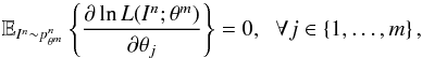 (6)then for any τn(·):Nn → Θ unbiased estimator of θm (i.e.,
  ) it follows that
 ![\begin{equation} \label{varcr} Var (\tau_n(I^n)_j) \geq [ \mathcal{I}_{\theta^m}(n)^{-1} ]_{j,j}, \end{equation}](/articles/aa/full_html/2016/10/aa28220-16/aa28220-16-eq49.png) (7)where ℐθm(n) is the Fisher information matrix given by
(7)where ℐθm(n) is the Fisher information matrix given by ![\begin{equation} \label{fisher} [ \mathcal{I}_{\theta^m}(n)]_{j,l} = \mathbb{E}_{I^n \sim p^n_{\theta^m}} \left\lbrace \frac{\partial \ln L(I^n; \theta^m)}{\partial \theta_j} \cdot \frac{\partial \ln L(I^n; \theta^m) }{\partial \theta_l} \right\rbrace, \end{equation}](/articles/aa/full_html/2016/10/aa28220-16/aa28220-16-eq51.png) (8)}∀j,l ∈ {1,...,m}. Returning to the observational problem in Sect. 2.1, Mendez et al. (2013, 2014) have characterized and analyzed the CR lower bound in Eq. (7) for the isolated problem of astrometry and photometry, respectively, as well as the joint problem of photometry and astrometry. For completeness, we highlight their 1-D astrometric result, which will be relevant for the discussion in subsequent sections of the paper:
(8)}∀j,l ∈ {1,...,m}. Returning to the observational problem in Sect. 2.1, Mendez et al. (2013, 2014) have characterized and analyzed the CR lower bound in Eq. (7) for the isolated problem of astrometry and photometry, respectively, as well as the joint problem of photometry and astrometry. For completeness, we highlight their 1-D astrometric result, which will be relevant for the discussion in subsequent sections of the paper:
Proposition 1. (Mendez et al. 2014, p. 800) Let us assume that and σ ∈ R+ are fixed and known, and we want to estimate xc (fixed but unknown) from a realization of In ~ pxc in Eq. (5), then the Fisher information in Eq. (8) is given by  (9)which from Eq. (7) induces a minimum variance bound for the astrometric estimation problem. More precisely
  (10)}The expression
  in Eq. (10) is a shorthand for the 1D astrometric CR lower bound in this parametric (classical) approach, as opposed to the Bayesian CR bound, which will be introduced in the next section.
3. The Bayesian estimation approach in astrometry
We now consider a Bayesian setting (Moon & Stirling 2000) for the problem of estimating the object location xc from a set of observations in ∈ Nn. The Bayes scenario considers that the (hidden) position is a random variable Xc (i.e., a random parameter), as opposed to a fixed although unknown parameter considered in the classical setting in Sect. 2.2. The goal is to estimate Xc from a realization of the observation random vector In. In order for this inference to be nontrivial, Xc and In should be statistically dependent. In our case this dependency is modeled by the observation equation in (5). More precisely, we have that the conditional probability of In given Xc is given by  (11)where L(in;xc) denotes the likelihood of observing in given that the object position is xc while pλk(xc)(ik) has been defined in Eq. (5).
The other fundamental element of the Bayesian approach is the “prior distribution” of Xc, given by a probability density function (pdf) ψ(·), i.e., for all B ⊂R,  (12)Consequently, in the Bayes setting we know that, for all A ⊂ Nn and B ⊂R, the joint distribution of the random vector (Xc,In) is given by
 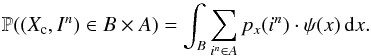 (13)It is important to highlight the role of the prior distribution of the object position Xc because it is the key mathematical object that allows us to pose the astrometry problem in the context of Bayesian estimation.
For the estimation of the object location, we need to establish the decision function τn(·):Nn →R that minimizes the MSE in inferring Xc from a realization of In. More precisely, the optimal decision would be the solution of the following problem: 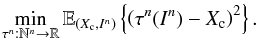 (14)The expectation value in Eq. (14) is taken with respect to the joint distribution of both variables (Xc,In) (see Eq. (13)), and the minimum is taken over all possible mappings (decision rules) from Nn to R. τn(In) in Eq. (14) is the estimation of Xc from In throughout the decision rule τn, also known as the estimator (Lehmann & Casella 1998). The optimal MSE estimator, which is the solution of Eq. (14), is known as the Bayes rule (or estimator), which for the square error risk function has a known theoretical solution function of the posterior density P(Xc = xc | In = in) (Kay 2010, chap. 8). More details are presented in Sect. 7 (see in particular Eq. (31)).
3.1. Bayes Cramér-Rao lower bound
As was the case in the parametric setting presented in Sect. 2.2, in the Bayes scenario it is also possible and meaningful to establish bounds for the minimum MSE (MMSE hereafter) in Eq. (14). This powerful result is known as the van Trees inequality or the Bayesian CR (BCR) lower bound:
Theorem 2. (Van Trees 2004, Sect. 2.4) For any possible decision rule τn:Nn →R, it is true that ![\begin{equation} \label{eq_sec_bayes_5} \mathbb{E}_{(X_{\rm c},I^n)} \left\{ \left( \tau^n(I^n)-X_{\rm c} \right)^2 \right\} \geq \left[ \mathbb{E}_{(I^n,X_{\rm c})} \left\{ \left( \frac{{\rm d} \ln \tilde{L}(X_{\rm c},I^n)}{{\rm d} x} \right)^2 \right\} \right]^{-1}, \end{equation}](/articles/aa/full_html/2016/10/aa28220-16/aa28220-16-eq77.png) (15)where
(15)where  (16)is shorthand for the joint density of (Xc,In) (see Eq. (13)), and where L(in;xc) is the likelihood of observing in given that the object position is xc, for all xc ∈R and in ∈ Nn (see Eq. (11)).
This result turns out to be the natural extension of the parametric CR lower bound to the Bayes setting (see Sect. 2.2). We note in particular the similarities between Eq. (15) and the expression in Eq. (7). In the Bayes setting this result offers a lower bound for the MSE of any estimator and, consequently, a lower bound for the MMSE, i.e., ![\begin{equation} \label{eq_sec_bayes_5b} \min_{\tau^n: \mathbb{N}^n \rightarrow \mathbb{R}} \mathbb{E}_{(X_{\rm c},I^n)} \left\{ \left( \tau^n(I^n)-X_{\rm c} \right)^2 \right\} \geq \left[ \mathbb{E}_{(X_{\rm c},I^n)} \left\{ \left( \frac{{\rm d} \ln \tilde{L}(X_{\rm c},I^n)}{{\rm d} x} \right)^2 \right\} \right]^{-1}\cdot \end{equation}](/articles/aa/full_html/2016/10/aa28220-16/aa28220-16-eq81.png) (17)
(17)
Proposition 2.
If we analyze what we call the Bayes-Fisher information (BFI) term (a function that depends on F and ψ) on the RHS of Eq. (17), we can establish that 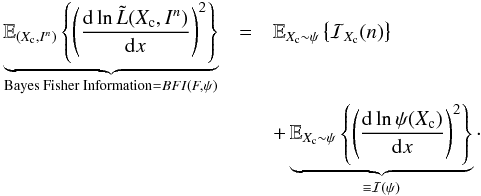 (18)(See Appendix A for the derivation of Eq. (18).)
From Eq. (18), we conclude that the BFI corresponds to the average Fisher information of the parametric setting (average with respect to ψ), plus a non-negative term associated with the prior distribution ψ that we call the “prior information” and denote ℐ(ψ). Finally, from Eq. (15) we have that 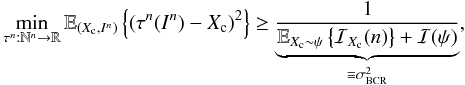 (19)which will be called the Bayesian CR (BCR) lower bound (compare to Eq. (10)).
3.2. Analysis and interpretation of the Bayes-Fisher information: BFI(F, ψ)
At this point it is interesting to analyze the BFI in Eq. (18), which reduces to the sum of two non-negative information components:  The first term, EXc ~ ψ{ℐXc(n)}, can be interpreted as the average information provided by the observations In to discriminate the random position Xc, which is precisely the average Fisher information of the parametric setting. We note, however, an important distinction: in the parametric setting, the CR lower bound depends directly on xc (see Eqs. (9) and (10)), whereas in the Bayesian setting the BCR does not depend on a specific value xc, but on a sort of prior average (over the position) function of the spatial sharpness of ψ(x). On the other hand, the second term on the RHS of Eq. (18), i.e., ℐ(ψ), can be interpreted as the information provided exclusively by the prior distribution ψ to decide Xc. This distinction is very important because it allows us to evaluate regimes where the prior information of the location for the source is relevant (or irrelevant), relative to the information provided by the observations. More precisely, we can say that
Definition 1. The prior information, ℐ(ψ), is said to be irrelevant relative to the observations, if  . Otherwise, it is said to be relevant.
Definition 2. The information of the observations, EXc ~ ψ{ℐXc(n)}, is said to be irrelevant relative to the prior distribution ψ, if  . Otherwise, it is said to be relevant.
4. Studying the gain in astrometric precision from the use of prior information
In this section we evaluate how much gain in performance can be obtained when we add prior information about the object position in the Bayes setting, with respect to the baseline parametric case where it is not possible to account for that information. It is clear that the knowledge of the distribution of Xc should provide a gain in the performance with respect to the parametric setting, where that information is either not available or not used. For this analysis, the performance bounds given by the CR bound in Eq. (10) and the BCR bound in Eq. (19) are compared.
We define the gain in performance, Gain(ψ), attributed to the prior distribution ψ, as the improvement in astrometric precision of the best estimator of the Bayes setting with respect to the best estimator of the parametric setting. In formal terms, the gain is given by the reduction in MSE (from the parametric to the Bayes setting) in the process of estimating Xc from In, i.e., 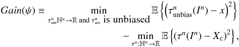 (20)where the first term on the RHS of Eq. (20) represents the minimum MSE over the family of unbiased estimators of the position (i.e., estimators that do not have access to ψ), while the second term on the RHS of Eq. (20) is the MMSE estimator of the Bayes setting, i.e. the best estimator over the family of mappings that have access to ψ. The next result establishes a tight lower bound for this gain, as a function of the information measures presented in Sect. 3.1.
Proposition 3. It follows that 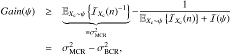 (21)where
  on the RHS of Eq. (21) denotes the average classical CR bound in Eq. (10). (see Appendix B for the derivation)
As was expected, this gain is an explicit function of ψ, and in particular, it is proportional to the prior information 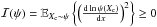 . One interesting scenario to analyze is the worse case prior that happens when Xc follows a uniform distribution over a bounded (compact) set. In this case, it is simple to show that
 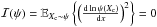 because a flat prior distribution does not carry any information regarding the location of the source and, consequently, Eq. (21) reduces to
  (22)The non-negativity of Gain(ψ), explicitly indicated in the last inequality of Eq. (22), follows from Jensen’s inequality (Perlman 1974) and from the fact that 1 /x is a convex function of x. This is a powerful result in favor of the Bayes approach, indicating that even for the worse prior, where the random parameter Xc is uniformly distributed and ℐ(ψ) = 0, the optimal Bayes rule offers a better MSE than the best unbiased parametric estimator, in other words, that
  for any prior. We also note the important fact that if ℐ(ψ) > 0 then Gain(ψ) > 0, from Eq. (21).
In the next section, we present a systematic analysis to evaluate and compare the classical vs. the Bayesian CR bounds and the gain Gain(ψ), for various concrete scenarios of astrometric estimation.
5. Evaluation of the performance bounds
In this section we quantify the gain in performance from the prior information under some realistic astrometric settings. To do this, we need to be more specific about the observation distribution in Eq. (5), and the prior distribution in Eq. (12).
5.1. Astrometric observational setting
Concerning the observation distribution, we adopt some realistic design variables and astronomical observing conditions to model the problem, similar to those adopted in Mendez et al. (2013, 2014). For the PSF (see Eq. (1)), various analytical and semi-empirical forms have been proposed, for instance the ground-based model in King (1971) and the space-based model in Bendinelli et al. (1987). For this analysis, we adopt a Gaussian PSF where  in Eq. (3), and where σ is the width of the PSF, assumed to be known. This PSF has been found to be a good representation for typical astrometric-quality ground-based data (Méndez et al. 2010). In terms of nomenclature,
  measured in arcsec, denotes the full width at half maximum (FWHM) parameter, which is an overall indicator of the image quality at the observing site (Chromey 2010).
The background profile, represented by  :k = 1,...,n } (see Eq. (2)), is a function of several variables, like the wavelength of the observations, the phase of the moon (which contributes significantly to the diffuse sky background, see Sect. 8), the quality of the observing site, and the specifications of the instrument itself. We consider a uniform background across the pixels underneath the PSF, i.e.,
  for all k. To characterize the magnitude of
  , it is important to first mention that the detector does not measure photon counts directly, but a discrete variable in Analog to Digital Units (ADUs) of the instrument, which is a linear proportion of the photon counts (Howell 2006). This linear proportion is characterized by a gain of the instrument G in units of e−/ADU. Here G is just a scaling value, where we can define
  and
and  as the intensity of the object and noise, respectively, in the specific ADUs of the instrument. Then, the background (in ADUs) depends on the pixel size Δx arcsec as (Mendez et al. 2013)
  (23)where fs is the diffuse sky background in ADU/arcsec, while D and RON, both measured in e−, model the dark-current and read-out noise of the detector on each pixel, respectively. We note that the first component on the RHS of Eq. (23) is attributed to the site, and its effect is proportional to the pixel size. On the other hand, the second component is attributed to errors of the PID, and it is pixel-size independent. This distinction is important when analyzing the performance as a function of the pixel resolution of the array (see details in Mendez et al. 2013, Sect. 4). More important is the fact that in typical ground-based astronomical observation, long exposure times are considered, which implies that the background is dominated by diffuse light coming from the sky (the first term on the RHS of expression (23)), and not from the detector (Mendez et al. 2013, Sect. 4). In this context, Mendez et al. (2013) have shown that
 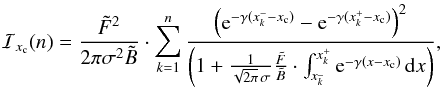 (24)where
  , with
  and
and  . Furthermore, in the so-called high-resolution regime, i.e., when Δx/σ ≪ 1, the following limiting (faint and bright source) closed-form expression for ℐxc(n) can be derived (see details in Mendez et al. 2013, Sect. 4.1.):
 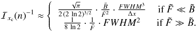 (25)Concerning the prior distribution, we consider a Gaussian distribution with mean μ and variance σpriori> 0, therefore
 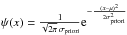 , for which,
 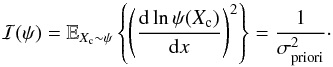 (26)Then, under these assumptions, the expression for the BCR lower bound for the astrometric problem in Eq. (19) becomes
 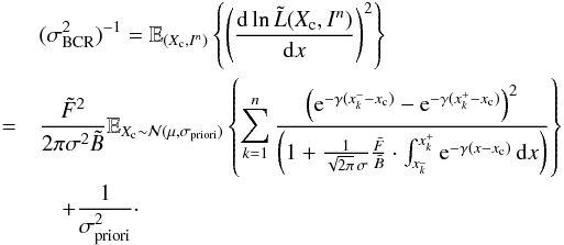 (27)This expression can be evaluated numerically if we know all the parameters of the problem, this is done in Sect. 5.3.
5.2. BCR lower bound at the high and low signal-to-noise regimes
Before evaluating the expression in expression (27), we can derive specialized closed-form expression for two relevant limiting scenarios in astrometry. First the scenario of a source dominated regime, when  (i.e., the estimation on a very bright object). For that we can fix the prior information σpriori> 0, , Δx, and FWHM, and take the limit when
  4. If we do so, it is simple to verify that the prior information becomes irrelevant (Definition 3) relative to the information of the observations In, and, consequently, the BCR bound in Eq. (27) reduces to
 ![\begin{eqnarray} \label{eq_sub_sec_bounds_analysis_5} \sigma^2_{\rm BCR}&=&\left[ \mathbb{E}_{X_{\rm c} \sim \mathcal{N}(\mu,\sigma_{\rm priori})} \left\{ \mathcal{I}_{X_{\rm c}}(n) \right\} \right]^{-1} \nonumber\\ &=& \left[\phantom{\frac{\left( {\rm e}^{-\gamma(x^-_k-x_{\rm c})} - {\rm e}^{-\gamma(x^+_k-x_{\rm c})} \right) ^2}{\left( 1 + \frac{1}{\sqrt{2 \pi} \, \sigma}\frac{\tilde{F}}{\tilde{B}} \cdot \int_{x^{\_}_k}^{x^+_k} {\rm e}^{-\gamma(x-x_{\rm c})} \, {\rm d}x \right)}}\hspace*{-4.3cm} \frac{\tilde{F}^2 }{2 \pi \sigma^2 \tilde{B}} \cdot \notag \right.\\ && \quad \mathbb{E}_{X_{\rm c} \sim \mathcal{N}(\mu,\sigma_{\rm priori})} \left.\left\{ \sum_{k=1}^{n} \frac{\left( {\rm e}^{-\gamma(x^-_k-x_{\rm c})} - {\rm e}^{-\gamma(x^+_k-x_{\rm c})} \right) ^2}{\left( 1 + \frac{1}{\sqrt{2 \pi} \, \sigma}\frac{\tilde{F}}{\tilde{B}} \cdot \int_{x^{\_}_k}^{x^+_k} {\rm e}^{-\gamma(x-x_{\rm c})} \, {\rm d}x \right)} \right\} \right]^{-1}\!\!\cdot \end{eqnarray}](/articles/aa/full_html/2016/10/aa28220-16/aa28220-16-eq137.png) (28)This is the case when the prior statistics of Xc does not have any impact on the performance of the estimation of the object location, because of the high fidelity (informatory content) of the observations.
(28)This is the case when the prior statistics of Xc does not have any impact on the performance of the estimation of the object location, because of the high fidelity (informatory content) of the observations.
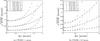 |
Fig. 1 Relationship between the classical MCR (from Eqs. (B.2) and (24)), and the BCR (from Eq. (27)) lower bounds as a function of pixel size for three different S/N regimes and two FWHM for the case of σpriori = 0.5 arcsec. As can be seen σBCR ≤ σMCR in all regimes. |
The second scenario is the background dominated regime, when  (i.e., the estimation on a very faint object). For this analysis we can fix σpriori> 0, , Δx, and the FWHM, and take the limit when
  5. In this case the information of the observation is irrelevant relative to the prior information ℐ(ψ) (Definition 4) and, consequently, the BCR bound in Eq. (27) reduces to
 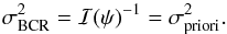 (29)Therefore, when the observations are irrelevant (non-informative), the MMSE of the estimation of Xc (Eq. (19)) reduces to the prior variance of Xc. Hence, it is direct to verify that the best MSE estimator (MMSE) in this context is the prior mean, i.e.,
 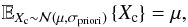 which, as expected, does not depend on the observations In.
We note that, in general, ℐ(ψ)-1 is an upper bound for the expression in Eq. (19), which represents the worse case scenario from the point of view of the quality of the observations.
5.3. Numerical evaluation and analysis
For the site conditions, we consider the scenario of a ground-based station located at a good site with clear atmospheric conditions and the specifications of current science-grade PIDs, where fs = 2 000 ADU/arcsec, D = 0, RON = 5 e−, G = 2 e−/ADU and FWHM = 0.5 arcsec or FWHM = 1 arcsec (with these values B = 313 ADU for Δx = 0.2 arcsec using Eq. (23)). In terms of scenarios of analysis, we explore different pixel resolutions for the PID array Δx ∈ [ 0.1,2.0 ] measured in arcsec, and different signal strengths F ∈ {268,540,1 612} ADU6. We note that increasing F implies increasing the signal-to-noise (S/N) of the problem, which can be approximately measured by the ratio F/B. On a given detector plus telescope setting, these different S/R scenarios can be obtained by changing appropriately the exposure time (open shutter) that generates the image (for further details, see Eq. (35)).
Figure 1 shows the parametric and Bayes CR bounds for three S/R regimes as a function of pixel size of the PID, and for two FWHM scenarios (0.5 and 1.0 arcsec). We first note, as the theory predicts, that the BCR bound is below the classical CR bound in all cases, and that the gap (the performance gain Gain(ψ) in Eq. (21)) increases as a function of increasing the pixel size in all cases. In fact the difference between the bounds becomes relevant for a pixel size larger than ~0.8 arcsec in Fig. 1a and bigger than ~0.6 arcsec in Fig. 1b. These results can be interpreted as follows: as Δx increases, the astrometric quality of the observation deteriorates and the prior information ℐ(ψ) becomes more and more relevant in the Bayes context, information that is not available in the parametric scenario. This explains the non-decreasing monotonic behavior of Gain(ψ) as a function of Δx for all the scenarios. If we look at one of the figures, and analyze the gain Gain(ψ) as a function of the S/N regime, we notice that the pixel size Δx at which the prior information ℐ(ψ) becomes relevant, in the sense that Gain(ψ) >τ for some fixed threshold τ, increases with the S/N. In other words, for faint objects the prior information is relevant for a wider range of pixel sizes, than in the case of bright objects.
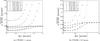 |
Fig. 3 Same as Fig. 1 but with σpriori = 0.05 arcsec. In this figure and in Fig. 2 we see that while σMCR increases without bound as the quality of the observations deteriorate, σBCR is bounded by the prior information in accordance with Eq. (29) (see also comments in the text after that equation). |
Figures 2 and 3 exhibit the trends for the bounds for the same experimental conditions as in Fig. 1, but with a significantly smaller prior variance (σpriori ∈ {0.1,0.05} arcsec). Therefore, we increase the prior information ℐ(ψ) to see what happens in the performance gain. In this scenario, the gain Gain(ψ) is significantly non-zero for all pixel resolutions, meaning that even for very small pixel size (in the range of 0.1-0.2 arcsec) the Bayes setting offers a boost in the performance, which is very significant for faint objects, see for instance the case of FWHM = 1 arcsec and S/N = 6 (Fig. 2a). From Figs. 2 and 3, another interesting observation is that the BCR bound converges to its upper bound limit, provided by the prior information  , as Δx increases, which is very clear in Fig. 3a for Δx> 1 in all the S/N regimes. We note that this upper bound limit is absent in the trend of the classical CR limit, as the performance of the best estimator in the parametric setting deteriorates with the loss of quality of the observations without a bound.
To conclude, we can say that having a source of prior information on the object position offers a gain in the performance of astrometry especially for faint objects, which can be substantial even for an excellent instrument (with a small noise and good pixel resolution) and optimum observational conditions (small background and small FWHM). On the other hand, when the observational conditions deteriorate, the Bayes setting becomes significantly better than the parametric approach for a wide range of object brightness. These curves provide a justification in favor of the use of the Bayes approach, in particular for the estimation of the position of faint objects. Therefore, if we have access to a source of prior information (e.g., a previous catalog), this can complement the information of the observations (fluxes) and introduce a gain in the performance of astrometry. The next section goes a bit deeper into this analysis, while Sect. 8 presents a simple comparison with a real catalog.
6. Equivalent object brightness
The information provided by the prior described in the previous sections can also be presented in the form of an equivalent (ficticious) increase in the flux of the source. If we have a non-zero prior information ℐ(ψ) > 0, and if we fix all the parameters associated with the observational conditions, i.e., Δx, FWHM, B, and G, what value should be given to the equivalent intensity Fpar of a fictitious object in the parametric (classical) estimation context (which has a true flux F) such that  (30)The BCR bound (derived from the Bayes-Fisher information, BFI), which are a function of F and ψ, have been defined in Eqs. (19) and (18) respectively, while
  denotes the average classical CR bound, function of the ficticious object with “equivalent” intensity Fpar and ψ (see the expression on the RHS of Eq. (B.2))7. In other words, for an object with true intensity F, we want to find the intensity of a brighter object Fpar in the parametric case (where the prior distribution ψ is not available) such that the classical CR and the BCR bound are the same. It is clear that Fpar ≥ F, and the difference is proportional to ℐ(ψ) > 08.
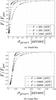 |
Fig. 4 Ratio of the flux for an object with true flux F and its equivalent flux Fpar obtained by the condition indicated in Eq. (30), as a function of the prior information given by σpriori. |
Figure 4a illustrates the ratio  as a function of the prior information
  . For this we consider three scenarios of object intensity F ∈ {200,500,1000} ADU, and we plot the ratio as a function of σpriori in the range [ 0,1 ] arcsec. As expected, when σpriori → ∞ then we have that
  ; on the other hand, when σpriori → 0 then
  . This last regime is more interesting to analyze, as it is the case when F is only a fraction of Fpar. In particular, at low S/N (panel a in Fig. 4), when the prior variance represented by σpriori is in the range of (0.05,0.1) arcsec, then F needs only to be between 20% and up to 50% smaller than Fpar, depending on the value of F, to yield the same astrometric CR bound. For this particular example another way of presenting this result is that a level of prior information σpriori ≤ 0.1 arcsec makes the object in a parametric context the equivalent of an object 1.25 to 2 times brighter (or, equivalently, a gain between 0.25 to 0.75 mag) than its real intensity when using a Bayesian approach. This is a remarkable observation, and provides a concrete way to measure the impact of prior information in astrometry. Figure 4b shows the case of brighter point sources, where σpriori needs to be significantly lower to observe the gains presented in Fig. 4a, as expected.
7. Comparing the BCR lower bound with the performance of the optimal Bayes estimator
One of the very important advantages of the Bayes estimation, in comparison with the parametric scenario, is that the solution of the MMSE estimator in Eq. (14), i.e., the Bayes rule, has an analytical expression function of the joint distribution of (Xc,In) that is available for this problem. In contrast, in the parametric scenario, there is no prescription on how to build an unbiased estimator that reaches the CR lower bound in Eq. (10), unless certain very restrictive conditions are met (see Mendez et al. 2013, especially their Eqs. (5) and (46)). Unfortunately these conditions are not satisfied in the astrometric case using PID detectors (see Lobos et al. (2015), especially their Sect. (3.1) and Appendix A), so in the parametric case there is no unbiased estimator that can precisely reach the CR bound.
Returning to our problem, the Bayes rule is the well-known posterior mean of Xc given a realization of the observations. More formally, for all in ∈ Nn the MMSE estimator is (Weinstein & Weiss 1988) 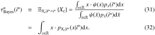 It should be noted that ψ(x)·px(in) is the joint density of the vector (Xc,In), the denominator of the RHS of Eq. (31) is the marginal distribution of In, which we denote by
  and, consequently,
  in Eq. (32) denotes the posterior density of Xc, evaluated at xc, conditioned to In = in.
Furthermore, the performance of the MMSE estimator  has the following analytical expression
 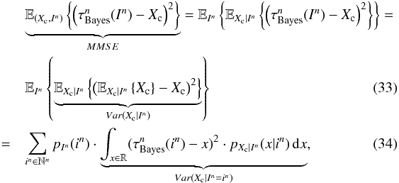 which can be interpreted as the average variance of Xc given realizations of In.
Therefore, revisiting the inequality in expression (19), it is essential to analyze how tight the BCR bound is or, equivalently, how large the difference between the MMSE in Eq. (34) and the BCR bound is. To answer this important question, in the next subsection we conduct some numerical experiments to evaluate how close the BCR bound is to the performance of the optimal estimator given by Eq. (34) under some relevant observational regimes, and in various scenarios of prior information.
7.1. Numerical results
Figures 5–7 present the MMSE from Eq. (34) side by side with the BCR bound in different observational regimes. From these results we can say that, for all practical purposes, the optimal Bayes rule in Eq. (32)(used to determine the location of a point source) achieves the BCR lower bound. Consequently, we conclude that for astrometry, the Bayes rule offers a concrete and implementable way to achieve the theoretical gain analyzed and studied in Sects. 4, 5.3, and 6 of this work.
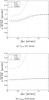 |
Fig. 5 Comparison between the MMSE from Eq. (34) and the BCR bound from Eq. (19) for two different σpriori scenarios, considering a S/N = 6. In addition, the MCR bound from Eq. (B.2) is plotted to highlight the information gain. |
8. An example of the BCR bound applied on real data
In this section we provide a simple example, based on real data, of how a priori information could be used to improve the quality of astrometric estimation.
8.1. Overall description of purpose
In Bayesian statistics, any piece of information that could be rendered in a mathematical form is in principle a possible prior. In the example we develop here, we use the positional information provided by a catalog that reports a (dependable) uncertainty on those positions. We assume that the catalog positions are distributed following a Gaussian distribution given by the reported uncertainty, centered on the catalog value (see Eq. (26)). Since the focus of this paper is on the uncertainty bounds and not on the estimation of the actual values (the coordinates) themselves, the catalog values are actually irrelevant. We will further assume that the prior values are not biased in any way, i.e., that there is no mismodeling (see also the paragraph above Eq. (B.1)) otherwise, combining the old and new values may render biased results (this issue, which is beyond the scope of the current paper, will be explored in a forthcoming report). Finally, we assume that we carry out new observations with pre-defined equipment (telescope+imaging camera) with known properties and under controlled conditions (FWHM, S/N at a certain flux), so that we will be able to evaluate the BCR and MCR bounds in Eq. (21) for each object in the catalog. If we fix the observational conditions, the only remaining free parameter is the distribution in flux of the observed objects (i.e., the apparent luminosity function). Since the goal of this example is to illustrate how the catalog data can have an impact on the expected quality of the positions derived from the new observations, we can compare the number of objects that satisfy a certain maximum positional uncertainty threshold as a function of brightness in the classical vs. the Bayesian approaches to illustrate the gains of the latter. A description of how do this, and the main results, are presented in the following sections.
8.2. Prior information and incremental observations
For the purposes outlined in the previous section, we will make use of the USNO-B1 catalog (Monet et al. 2003) which provides astrometric positions and their uncertainties, and photographic photometry on various optical bands for a complete set of stars brighter than V ~ 21 with an overall 0.2 arcsec astrometric accuracy at J2000 and ~0.3 mag photometric accuracy. In addition, for each entry the catalog provides a star/galaxy index, which is believed to be 85% accurate at distinguishing stars from non-stellar sources. In order to have a clear star/galaxy separation and the best possible photometry, both of which become less accurate in dense stellar regions, we have extracted a representative area of 20 × 20 arc-minutes2 around the SGP from the online version of the catalog available through the VizierR web page within the CDS service9.
Our test catalog contains 2700 entries of which 226 objects satisfy the joint criteria that their star/galaxy index is ≥5 (and are thus considered to be stars to a high level of certainty) and that have valid values for their photometry (i.e., B or R mag ≠ 99.9910) and their astrometry (σRA ≠ 999, σDEC ≠ 999). Since the purpose of this exercise is to illustrate the impact of prior information (provided in this case by the USNO-B1 catalog), we further trimmed the sample to those objects with a slightly smaller (but still realistic) uncertainty threshold in their astrometric positions equal to 0.1 arcsec (because our analysis has been done for a linear array, we are considering only one coordinate, with an uncertainty which is the mean of the values declared in the catalog for RA cos(Dec) and Dec coordinates). This sample contains 106 objects, and their histogram as a function of brightness is depicted in Fig. 8. We have chosen this astrometric uncertainty threshold as a value useful for fiber-fed or multi-slit target positioning in typical spectrographs. We will now evaluate how these histograms change through new observations when we incorporate the prior information.
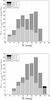 |
Fig. 8 Histogram of the number of stars (in bins of 1 mag) in an area of 20 × 20 arc-min2 towards the SGP from the USNO-B1 catalog that satisfy the criteria that their astrometric position has a positional uncertainty less that a threshold value of σcrit = 0.1 arcsec. Light gray is for those objects that satisfy the astrometric threshold in the catalog directly (106 objects). Light+dark gray is the number of objects that would satisfy the criteria when one observation with EFOSC2@NTT is carried out on the same sample, according to the expectations from the classical MCR, for a FWHM of 0.7 arcsec. Finally, light+dark gray+black is the number of objects when the BCR is considered (in this case σpriori is the catalog value for the positional uncertainty of each individual object). The upper panel is for the R band, lower panel for the B band. |
We assume that we obtain new astrometric observations with a typical optical imaging PID. As a representative case we have taken the throughput and other specifications of the EFOSC2 instrument (with CCD#40) currently installed at the NTT 3.58 m telescope of the ESO-La Silla observatory11. In particular, we adopt a RON of 9.2 e− (normal read-out mode), a (negligible) dark current D = 7 e−/pix/h, a gain G = 1.33 e−/ADU, and an effective pixel size (in 2 × 2 binned mode) of Δx = 0.24 arcsec. The throughput of EFOSC2 at the NTT is constantly monitored12, and these “zero points” (on different pass bands) are used to compute the flux (in e−/s) for objects of a given apparent magnitude as observed by EFOSC2, but also to estimate the flux that would be observed by telescopes of other aperture (of similar optical characteristics as the NTT), or through detectors of different pixel size (of similar characteristics to CCD#40), as explained below.
To fully incorporate the background fs (see Eq. (23)) in our CR estimations, we need to consider its main contributor, i.e., the changing sky brightness according to moon phase. For this we use the table of sky brightness in mag/arcsec2 at different pass bands and different moon ages provided by Walker (1987); although it was measured for the sky above CTIO, it can be taken as representative for a good astronomical site. Our calculations turned out to be rather insensitive to moon phase, mostly because of the relatively bright magnitude limit of the USNO-B1 catalog, and we therefore adopted in what follows a moon age of 7 days (gray time) corresponding to a sky brightness of 21.6 mag arcsec-2 in the B band and 20.6 mag arcsec-2 in the R band.
We also assume that our new observations are carried out in such a way that we are able to secure a minimum S/N of 3.0 for the faintest objects available in our SGP sample from the USNO-B1 catalog. This defines an exposure time t that is the solution of the equation (see also Mendez et al. 2013, their Eq. (28)) 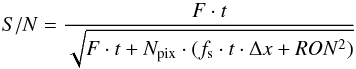 (35)where F is the flux in e−/s of the faintest USNO-B1 sources as seen by EFOSC2@NTT, Npix is the number of pixels under the (chosen) aperture for computing the flux under the PSF (we adopt Npix such that the S/N includes 99.5% of the source flux), while the other terms have all been previously defined. With the derived exposure time, we discard any catalog object for which the peak count is predicted to be larger than the detector saturation level of 65 535 ADUs. This eliminates a few objects in our histograms with B, R ≤ 11.
8.3. Analysis of MCR and BCR predictions
If we secure one observation with the exposure time calculated from Eq. (35) at the NTT, and if we assume that the uncertainty of their astrometric positions tightly approach the theoretical limits (which is justified by our results in Sect. 7.1), then the number of targets (effectively available on the sky, since they are on the USNO-B1 catalog) whose positional uncertainty is smaller than the adopted threshold of 0.1 arcsec would increase, as shown by the light+dark gray areas in Fig. 8. To compute the CR bounds we have assumed a FWHM = 0.7 arcsec. Obviously, the NTT data are predicted to be of much higher astrometric quality than the data derived from the plates, which is clearly seen as the significant increase in the number of sources that satisfy the astrometric threshold σcrit. Finally, in black, we show the number of sources that would be added to the light+dark gray histogram, as a function of magnitude, if we compute the BCR, i.e., incorporating the prior information from the catalog. In this case, the prior information does not play a significant role as the increase in the number of sources is minimal. This shows again that since the NTT data alone is of much higher quality, the information contained in the catalog is less relevant.
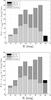 |
Fig. 9 Similar to Fig. 8, except that both panels are in the R band. The upper panel is for EFOSC2@NTT with a degraded seeing of 1.2 arcsec FWHM, while the lower panel is for optimistic sky conditions of 0.7 arcsec but on a 1 m class telescope equipped with a camera equivalent to EFOSC2. These histograms show the evolving role of the a priori information in improving the astrometry depending on sky conditions and the equipment used. The benefits of using the Bayesian approach is noticeable at the faintest bins. |
A scenario where we consider an observation at the NTT under less favorable sky conditions (FWHM = 1.2 arcsec) is shown in the left panel of Fig. 9. Compared to the upper panel of Fig. 8 we see that the two faintest bins do benefit from the prior position, as expected. If we insist on sharp images, but now using a smaller aperture telescope of 1 m (in comparison with the 3.58 m of the NTT), the predicted behavior will be that of Fig. 9 (lower panel). This last case is interesting: While in most apparent magnitude bins the contribution from the current observations almost doubles the number of targets per bin in comparison with the objects from USNO-B1 that satisfy the positional threshold, the impact of the Bayesian CR in the faintest bin is most significant. This result is in line with the gains for faint targets described in Sects. 5.3 and 6, and shown in Figs. 1 to 4.
Finally, two cases (which are perhaps more realistic) are presented in Fig. 10 but utilizing a 1 m telescope for a moderate seeing (upper panel) and a less-than-ideal seeing (lower panel). As the image quality of the new observations deteriorates, we can see that the contribution of these observations to the number of objects with good astrometric positions decreases, while the use of prior information reinforces even further the faintest bins. For example, in Fig. 10a, the overall number of objects with good astrometry increases by about 9% when using the BCR (or 12% for Fig. 10b), although the increase is quite dramatic at the lowest S/N bins (see Fig. 10 caption).
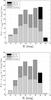 |
Fig. 10 Similar to Fig. 9, except that both panels are the predictions for observations with a 1 m class telescope. The upper panel is for a FWHM of 1.2 arcsec, while the lower panel is for a FWHM of 2.0 arcsec. As the quality of the new observations degrades, their contribution to the sample, as well as that using prior information, is displaced to brighter magnitudes. The gain from using the information in the catalog is relevant in both cases at the faintest bins, as in Fig. 9: at 19th magnitude we have 38 objects in the Bayesian scenario, and 25 objects in the parametric approach, i.e., an increase of more than 50% for the upper panel. In the lower panel the increase is even more important: 23 objects in the Bayesian approach and 12 from the catalog (equal to the number from MCR), an increase of ~90%. |
We note that in all the computations above, we have taken the catalog as is, but we know that in the faintest bins, the real number of targets will be larger than shown in Figs. 8 to 10 due to incompleteness. However, since these objects are not in the catalog, and hence there is no prior information on them, they do not affect the impact that prior information has on their positions, which was the purpose of this exercise (the minimum astrometry uncertainty for these extra objects will be solely determined by their classical MCR).
8.4. Improvements in the mean errors of individual positions
In the previous section, we give an overview of the impact of using a priori information on starcounts as a function of magnitude when we impose a constraint on the minimum acceptable astrometric accuracy. This is relevant for the evaluation of the bulk performance of surveys that convey astrometric information, but for a practitioner astrometrist, it might be more relevant to be able to evaluate the actual improvement in astrometric precision of the catalogued objects using the BCR in comparison with the classical MCR. In what follows we present this information for the same observational scenarios described in the previous section, giving more details on the expected improvement in the mean error of individual positions.
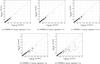 |
Fig. 11 BCR vs. MCR bounds for the whole SGP sample analyzed in this paper. The dashed line indicates the one-to-one relationship, i.e., no gain of the BCR with respect to the parametric case given by the MCR bound. |
In Fig. 11 we show the BCR vs. the MCR bounds (both in arcsec) for all of the 226 objects in the USNO-B1 stellar-like SGP catalog described above. The diagonal dashed line indicates the locus of objects for which the use of a Bayesian approach does not lead to any improvement over the classical parametric case. As explained in Proposition 3, Eq. (22), and in Sect. 5.2, we predict that all the objects will be located below that line or, at most, on the line, which is obviously the case in all the observational scenarios. As was already hinted in the histograms presented in the previous section, when the (new) observations become of poorer and poorer quality or, equivalently, when the a priori information becomes more and more relevant (in the precise sense defined in Sect. 3.2), a larger number of objects start to populate the bottom of these σBCR vs. σMCR diagrams. The two objects that appear below the line even in the case when the observations are of good quality (see in particular panels a–c in Fig. 11) have very high quality positions reported on the catalog and therefore, for them, the a priori information is quite relevant, always. Another important point to highlight from these plots is that, of course, as the quality of the observations deteriorate, both the σMCR and σBCR increase, which pushes the catalog objects up and to the right in the diagrams. However, the use of the Bayesian approach ensures that the deterioration of the latter is hampered by the use of a priori information, which the MCR does not use, hence this explains the increased scattering of points to the right and below the diagonal line from panels a–e in Fig. 11.
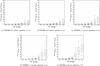 |
Fig. 12 Fractional improvement of astrometric precision as a function brightness in the R band for the whole SGP USNO-B1 sample, in centered 1 mag bins, for the different observational scenarios presented in the previous section. The box boundary indicates the 1st and 3rd quartiles, the horizontal line in the center of the box is the median, and the upper and lower ticks show respectively the largest and smallest value in that magnitude bin. |
As clearly shown by Figs. 5–7 in Sect. 7.1, an underlying parameter determining the gains of the Bayesian approach is the source flux, which is not well rendered by Fig. 11. To address more clearly this particular aspect, Fig. 12 shows the relative improvement on astrometric precision as a function of magnitude for the whole USNO-B1 SGP sample. This improvement is measured in terms of a relative gain in astrometric performance, i.e., for each sample of the database we compute  . This array of figures ratifies the usefulness of a Bayesian strategy to mitigate the inevitable deterioration of astrometric precision as a function of flux (see Eq. (30) in Mendez et al. 2014). Remarkably, this becomes particularly dramatic when the observations are performed under adverse conditions (panels d and e in Fig. 12), where one can expect improvements of between 10% and 50% in the astrometric precision for the faintest objects when using the Bayesian approach as described here.
9. Conclusions and outlook
In this work we provide a systematic analysis of the best precision that can be achieved to determine the location of a stellar-like object on a CCD-like detector array in a Bayesian setting. This setting changes in a radical way the nature of the inference task in hand: from a parametric context – in which we are estimating a constant (or parameter) from a set of observations – to a setting in which we estimate a random object (i.e., the position is modeled as a random variable) from observations that are statistically dependent with the position. A key new element of the Bayesian setting is the introduction of a prior distribution of the object position: we systematically quantify and analyze the gain in astrometric performance from the use of a prior distribution of the object position, information which is not available (or used) in the classical parametric setting. We tackle this problem from a theoretical and experimental point of view.
We derive new closed-form expressions for the Bayesian CR and expressions to estimate the gain in astrometric precision. Different observational regimes are evaluated to quantify the gain induced from the prior distribution of the object position. An insightful corollary of this analysis is that the Bayes setting always offers a better performance than the parametric setting, even in the worse-case prior (i.e., that of a uniform distribution).
We evaluate numerically the benefits of the Bayes setting with respect to the parametric scenario under realistic experimental conditions: we find that the gain in performance is significant for various observational regimes, which is particularly clear in the case of faint objects, or when the observations are taken in poor conditions (i.e., in the low signal-to-noise regime). In this context we introduce the new concept of the equivalent object brightness. We also submit evidence that the MMSE estimator of this problem (the well-known conditional mean) tightly achieves the Bayesian CR lower bound, a remarkable result, demonstrating that all the performance gains presented in the theoretical analysis part of our paper can indeed be achieved with the MMSE estimator, which has in principle a practical implementation. We finalize our paper with a simple example of what could be achieved using the Bayesian approach in terms of the astrometric precision of positional measurements with new observations of varying quality, when we incorporate data from existing catalog as prior information.
In a forthcoming paper we expect to extend the present analysis of the BCR to the case of photometric estimations and to implement the MMSE estimator in Eq. (31). With the help of simulations we will be able to quantify the gains (and risks) of using a Bayesian approach with priors for the joint estimation of photometry and astrometry of point sources. For example, Michalik et al. (2015b) have pointed out that a Bayesian approach would lead to biased astrometric results (particularly for proper motions and parallaxes), and should be avoided if a reasonable solution can be found using a parametric approach. The conditions and extent to which this statement is true could be precisely verified through detailed simulations, thus providing a range where a Bayesian scheme might be safely applied.
This analysis can be generalized to the 2D case as shown in Mendez et al. (2013).
Throughout this paper, in general, capital letters (e.g., In) denote a random variable (or, in this case, a random vector of n elements), and lower-case letters (e.g., in) denote a particular realization (or measured value) of the variable. This distinction will become particularly important in the Bayesian context described in the next section.


These are the same values explored in Mendez et al. (2013, Table 3).
This comes from the fact that  in Eq. (B.4).
These can be found in the Observatory web pages: http://www.eso.org/sci/facilities/lasilla/instruments/efosc.html
In Sect. 7.1 we show that this hypothesis is indeed true for many realistic astrometric scenarios.
Acknowledgments
This material is based on work supported by grant of CONICYT-Chile, Fondecyt 1140840. In addition, the work of J. F. Silva and M. Orchard is supported by the Advanced Center for Electrical and Electronic Engineering, Basal Project FB0008. R.A.M. and J.F.S. acknowledge support from a CONICYT-Fondecyt grant # 1151213, and R.A.M. from the Project IC120009 Millennium Institute of Astrophysics (MAS) of the Iniciativa Científica Milenio del Ministerio de Economía, Fomento y Turismo de Chile. R.A.M. also acknowledges ESO/Chile for hosting him during his sabbatical leave during 2014, the period in which part of this work was started. This research has made use of the VizieR catalog access tool, CDS, Strasbourg, France. The original description of the VizieR service was published in Ochsenbein et al. (2000).
References
- Adorf, H.-M. 1996, in ADASS, 101, 13 [Google Scholar]
- Auer, L., & Van Altena, W. 1978, AJ, 83, 531 [NASA ADS] [CrossRef] [Google Scholar]
- Bastian, U. 2004, 2004BASNOCODE, Gaia DPAC Public Documents, http://www.cosmos.esa.int/web/gaia/public-dpac-documents [Google Scholar]
- Bendinelli, O., Parmeggiani, G., Piccioni, A., & Zavatti, F. 1987, AJ, 94, 1095 [NASA ADS] [CrossRef] [Google Scholar]
- Bouquillon, S., Mendez, R., Altmann, M., et al. 2016, A&A submitted [Google Scholar]
- Chromey, F. R. 2010, To measure the sky: an introduction to observational astronomy (Cambridge University Press) [Google Scholar]
- Cramér, H. 1946, Scandinavian Actuarial J., 1946, 85 [Google Scholar]
- Freyhammer, L. M., Andersen, M. I., Arentoft, T., Sterken, C., & Nørregaard, P. 2001, Exp. Astron., 12, 147 [NASA ADS] [CrossRef] [Google Scholar]
- Gawiser, E., van Dokkum, P. G., Herrera, D., et al. 2006, ApJS, 162, 1 [NASA ADS] [CrossRef] [Google Scholar]
- Gray, R. M., & Davisson, L. D. 2004, An introduction to statistical signal processing (Cambridge University Press) [Google Scholar]
- Høg, E. 2011, Balt. Astron., 20, 221 [NASA ADS] [Google Scholar]
- Howell, S. B. 2006, Handbook of CCD astronomy (Cambridge University Press), 5 [Google Scholar]
- Jakobsen, P., Greenfield, P., & Jedrzejewski, R. 1992, A&A, 253, 329 [NASA ADS] [Google Scholar]
- Kay, S. M. 2010, Fundamentals of statistical signal processing: estimation theory (Prentice-Hall PTR) [Google Scholar]
- King, I. R. 1971, PASP, 83, 199 [NASA ADS] [CrossRef] [Google Scholar]
- Lee, J.-F., & van Altena, W. 1983, AJ, 88, 1683 [NASA ADS] [CrossRef] [Google Scholar]
- Lehmann, E. L., & Casella, G. 1998, Theory of point estimation, (Springer Science & Business Media), 31 [Google Scholar]
- Lindegren, L. 1978, in IAU Colloq. 48: Modern Astrometry, 1, 197 [Google Scholar]
- Lindegren, L. 2008, GAIA-C3-TN-LU-LL-078, Gaia DPAC Public Documents, http://www.cosmos.esa.int/web/gaia/public-dpac-documents [Google Scholar]
- Lindegren, L. 2010, ISSI Sci. Rep. Ser., 9, 279 [Google Scholar]
- Lobos, R. A., Silva, J. F., Mendez, R. A., & Orchard, M. 2015, PASP, 127, 1166 [NASA ADS] [CrossRef] [Google Scholar]
- Mason, E. 2008, in The 2007 ESO Instrument Calibration Workshop, eds. A. Kaufer, & F. Kerber (Springer-Verlag), 107 [Google Scholar]
- Méndez, R. A., Costa, E., Pedreros, M. H., et al. 2010, PASP, 122, 853 [NASA ADS] [CrossRef] [Google Scholar]
- Mendez, R. A., Silva, J. F., & Lobos, R. 2013, PASP, 125, 580 [NASA ADS] [CrossRef] [Google Scholar]
- Mendez, R. A., Silva, J. F., Orostica, R., & Lobos, R. 2014, PASP, 126, 798 [NASA ADS] [Google Scholar]
- Michalik, D., & Lindegren, L. 2016, A&A, 586, A26 [NASA ADS] [CrossRef] [EDP Sciences] [Google Scholar]
- Michalik, D., Lindegren, L., Hobbs, D., & Lammers, U. 2014, A&A, 571, A85 [NASA ADS] [CrossRef] [EDP Sciences] [Google Scholar]
- Michalik, D., Lindegren, L., & Hobbs, D. 2015a, A&A, 574, A115 [NASA ADS] [CrossRef] [EDP Sciences] [Google Scholar]
- Michalik, D., Lindegren, L., Hobbs, D., & Butkevich, A. G. 2015b, A&A, 583, A68 [NASA ADS] [CrossRef] [EDP Sciences] [Google Scholar]
- Mignard, F. 2009, GAIA-C3-TN-OCA-FM-040, Gaia DPAC Public Documents, http://www.cosmos.esa.int/web/gaia/public-dpac-documents [Google Scholar]
- Monet, D. G., Levine, S. E., Canzian, B., et al. 2003, AJ, 125, 984 [NASA ADS] [CrossRef] [Google Scholar]
- Moon, T. K., & Stirling, W. C. 2000, Mathematical methods and algorithms for signal processing (Upper Saddle River: Prentice Hall), 1 [Google Scholar]
- Ochsenbein, F., Bauer, P., & Marcout, J. 2000, A&A, 143, 23 [Google Scholar]
- Perlman, M. D. 1974, J. Multivariate Analysis, 4, 52 [CrossRef] [Google Scholar]
- Rao, R. C. 1945, Bulletin of the Calcutta Mathematical Society, 37, 81 [Google Scholar]
- Tyson, J. A. 1986, J. Opt. Soc. Am. A, 3, 2131 [NASA ADS] [CrossRef] [Google Scholar]
- van Altena, W., & Auer, L. 1975, in Image Processing Techniques in Astronomy (Springer), 411 [Google Scholar]
- Van Trees, H. L. 2004, Detection, estimation, and modulation theory (John Wiley & Sons) [Google Scholar]
- Walker, A. 1987, NOAO Newsletter, 10, 16 [Google Scholar]
- Weinstein, E., & Weiss, A. J. 1988,IEEE Transactions on Information Theory, 34, 338 [Google Scholar]
- Winick, K. A. 1986, J. Opt. Soc. Am. A, 3, 1809 [NASA ADS] [CrossRef] [Google Scholar]
Appendix A: Derivation of the Bayes-Fisher information identity in Eq. (18)
Using the definition of  in Eq. (16), it follows that
 ![\appendix \setcounter{section}{1} \begin{eqnarray} \label{eq:app_derivation_bfi_identity_1} &&\mathbb{E}_{(X_{\rm c},I^n)} \left\{ \left( \frac{{\rm d} \ln \tilde{L}(X_{\rm c}, I^n)}{{\rm d} x} \right)^2 \right\} = \mathbb{E}_{(X_{\rm c},I^n)} \left\{ \left( \frac{{\rm d} \ln L(I^n; X_{\rm c})}{{\rm d} x} \right)^2 \right\} \nonumber\\[1mm] && + 2\cdot \mathbb{E}_{(X_{\rm c},I^n)} \left\{ \frac{{\rm d} \ln L(I^n; X_{\rm c})}{{\rm d} x} \cdot \frac{{\rm d} \ln \psi(X_{\rm c})}{{\rm d}x} \right\} + \mathbb{E}_{X_{\rm c}} \left\{ \left( \frac{{\rm d} \ln \psi(X_{\rm c})}{{\rm d}x} \right)^2\right\}\\[1mm] \label{eq:app_derivation_bfi_identity_1b} &=& \mathbb{E}_{X_{\rm c}} \underbrace{\mathbb{E}_{I^n|X_{\rm c}} \left\{ \left( \frac{{\rm d} \ln L(I^n; X_{\rm c})}{{\rm d} x} \right)^2 \right\}}_{\mathcal{I}_{X_{\rm c}}(n)} + \mathbb{E}_{X_{\rm c}} \left\{ \left( \frac{{\rm d} \ln \psi(X_{\rm c})}{{\rm d}x} \right)^2\right\}\\[1mm] \label{eq:app_derivation_bfi_identity_1c} &=& \mathbb{E}_{X_{\rm c}} \left\{ \mathcal{I}_{X_{\rm c}}(n) \right\} + \mathbb{E}_{X_{\rm c}} \left\{ \left( \frac{{\rm d} \ln \psi(X_{\rm c})}{{\rm d}x} \right)^2\right\}\cdot~~~~~~~~~~~~~~~~~~~~~~~~~~~~ \end{eqnarray}](/articles/aa/full_html/2016/10/aa28220-16/aa28220-16-eq223.png) The first line, Eq. (A.1), comes from the definition of
The first line, Eq. (A.1), comes from the definition of  in Eq. (16). The second line, Eq. (A.2), follows directly from the fact that for every position xc ∈R,
  (see Eq. (6)). The last line, Eq. (A.3), results from the definition of the Fisher information for the scalar case in Eq. (8).
Appendix B: Proof of the lower bound of Gain(ψ) in Eq. (21)
Proof: let us consider a fixed prior distribution ψ. To evaluate the performance of the baseline parametric case, let us consider an arbitrary unbiased estimator τn(·) of the position. Then, conditioned on a position Xc = x, we have that  , this from the fact that the estimator is unbiased. Therefore, from the CR lower bound in Sect. 2.2, it follows that
  (B.1)
(B.1)
From the expression above, the average performance of τn(·), with respect to the statistics of Xc ~ ψ, is not smaller than  , which is the average CR lower bound (with respect to ψ). In other words, for any unbiased estimator
  of the object position (
 denotes the collection of unbiased estimator), we have that
  (B.2)We note that is the average classical CR bound, which, as we see below (Eq. (B.4)), is the right figure of merit to compare with the Bayesian CR lower bound. In other words, Eq. (B.2) offers a lower bound for the MSE of any unbiased estimator with no access to the prior probability law of Xc.
On the other hand, we have that using the prior distribution of Xc, the BCR on Eq. (19) offers a lower bound for the MSE of any estimator. If we assume for a moment that the optimal MSE estimator solution of Eq. (14), which we denote by  , achieves the BCR lower bound13 in Eq. (19), then we can compute the performance gain as follows:
 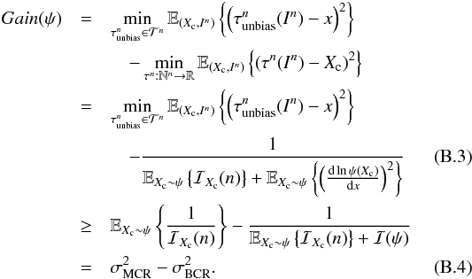 The first equality is from definition, the second equality is from the assumption that achieves the BCR bound, and the last inequality is from Eq. (B.2). This concludes the result.
All Figures
|
Fig. 1 Relationship between the classical MCR (from Eqs. (B.2) and (24)), and the BCR (from Eq. (27)) lower bounds as a function of pixel size for three different S/N regimes and two FWHM for the case of σpriori = 0.5 arcsec. As can be seen σBCR ≤ σMCR in all regimes. |
| In the text | |
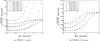 |
Fig. 2 Same as Fig. 1 but with σpriori = 0.1 arcsec. |
| In the text | |
|
Fig. 3 Same as Fig. 1 but with σpriori = 0.05 arcsec. In this figure and in Fig. 2 we see that while σMCR increases without bound as the quality of the observations deteriorate, σBCR is bounded by the prior information in accordance with Eq. (29) (see also comments in the text after that equation). |
| In the text | |
|
Fig. 4 Ratio of the flux for an object with true flux F and its equivalent flux Fpar obtained by the condition indicated in Eq. (30), as a function of the prior information given by σpriori. |
| In the text | |
|
Fig. 5 Comparison between the MMSE from Eq. (34) and the BCR bound from Eq. (19) for two different σpriori scenarios, considering a S/N = 6. In addition, the MCR bound from Eq. (B.2) is plotted to highlight the information gain. |
| In the text | |
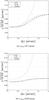 |
Fig. 6 Same as Fig. 5 but considering S/N = 12. |
| In the text | |
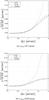 |
Fig. 7 Same as Fig. 5 but considering S/N = 32. |
| In the text | |
|
Fig. 8 Histogram of the number of stars (in bins of 1 mag) in an area of 20 × 20 arc-min2 towards the SGP from the USNO-B1 catalog that satisfy the criteria that their astrometric position has a positional uncertainty less that a threshold value of σcrit = 0.1 arcsec. Light gray is for those objects that satisfy the astrometric threshold in the catalog directly (106 objects). Light+dark gray is the number of objects that would satisfy the criteria when one observation with EFOSC2@NTT is carried out on the same sample, according to the expectations from the classical MCR, for a FWHM of 0.7 arcsec. Finally, light+dark gray+black is the number of objects when the BCR is considered (in this case σpriori is the catalog value for the positional uncertainty of each individual object). The upper panel is for the R band, lower panel for the B band. |
| In the text | |
|
Fig. 9 Similar to Fig. 8, except that both panels are in the R band. The upper panel is for EFOSC2@NTT with a degraded seeing of 1.2 arcsec FWHM, while the lower panel is for optimistic sky conditions of 0.7 arcsec but on a 1 m class telescope equipped with a camera equivalent to EFOSC2. These histograms show the evolving role of the a priori information in improving the astrometry depending on sky conditions and the equipment used. The benefits of using the Bayesian approach is noticeable at the faintest bins. |
| In the text | |
|
Fig. 10 Similar to Fig. 9, except that both panels are the predictions for observations with a 1 m class telescope. The upper panel is for a FWHM of 1.2 arcsec, while the lower panel is for a FWHM of 2.0 arcsec. As the quality of the new observations degrades, their contribution to the sample, as well as that using prior information, is displaced to brighter magnitudes. The gain from using the information in the catalog is relevant in both cases at the faintest bins, as in Fig. 9: at 19th magnitude we have 38 objects in the Bayesian scenario, and 25 objects in the parametric approach, i.e., an increase of more than 50% for the upper panel. In the lower panel the increase is even more important: 23 objects in the Bayesian approach and 12 from the catalog (equal to the number from MCR), an increase of ~90%. |
| In the text | |
|
Fig. 11 BCR vs. MCR bounds for the whole SGP sample analyzed in this paper. The dashed line indicates the one-to-one relationship, i.e., no gain of the BCR with respect to the parametric case given by the MCR bound. |
| In the text | |
|
Fig. 12 Fractional improvement of astrometric precision as a function brightness in the R band for the whole SGP USNO-B1 sample, in centered 1 mag bins, for the different observational scenarios presented in the previous section. The box boundary indicates the 1st and 3rd quartiles, the horizontal line in the center of the box is the median, and the upper and lower ticks show respectively the largest and smallest value in that magnitude bin. |
| In the text | |
Current usage metrics show cumulative count of Article Views (full-text article views including HTML views, PDF and ePub downloads, according to the available data) and Abstracts Views on Vision4Press platform.
Data correspond to usage on the plateform after 2015. The current usage metrics is available 48-96 hours after online publication and is updated daily on week days.
Initial download of the metrics may take a while.