| Issue |
A&A
Volume 593, September 2016
|
|
|---|---|---|
| Article Number | A133 | |
| Number of page(s) | 17 | |
| Section | Stellar structure and evolution | |
| DOI | https://doi.org/10.1051/0004-6361/201628459 | |
| Published online | 05 October 2016 | |
New spectroscopic binary companions of giant stars and updated metallicity distribution for binary systems⋆
1 Departamento de Astronomía, Pontificia Universidad Católica, Av.Vicuña Mackenna 4860, 782-0436 Macul, Santiago, Chile
e-mail: pvbluhm@uc.cl
2 Center of Astro-Engineering UC, Pontificia Universidad Católica, 7820436 Macul, Santiago, Chile
3 Department of Electrical Engineering, Pontificia Universidad Católica, 7820436 Macul, Santiago, Chile
4 Departamento de Astronomía, Universidad de Chile, Camino El Observatorio 1515, Las Condes, Santiago, Chile
5 Instituto de Física y Astronomía, Universidad de Vaparaíso, Cassila 5030, Valparaíso, Chile
6 School of Physics and Australian Centre for Astrobiology, University of New South Wales, 2052 Sydney, Australia
7 Computational Engineering and Science Research Centre, University of Southern Queensland, 4350 Toowoomba, Australia
8 Departamento de Ciencias Fisicas, Universidad Andres Bello, Avda. Republica 252, Santiago, Chile
9 Millennium Institute of Astrophysics, Santiago, Chile
10 Departamento de Astronomía, Universidad de Concepción, Casilla 160- C Concepción, Chile
11 European Southern Observatory, Casilla 19001, Santiago, Chile
Received: 8 March 2016
Accepted: 28 June 2016
We report the discovery of 24 spectroscopic binary companions to giant stars. We fully constrain the orbital solution for 6 of these systems. We cannot unambiguously derive the orbital elements for the remaining stars because the phase coverage is incomplete. Of these stars, 6 present radial velocity trends that are compatible with long-period brown dwarf companions. The orbital solutions of the 24 binary systems indicate that these giant binary systems have a wide range in orbital periods, eccentricities, and companion masses. For the binaries with restricted orbital solutions, we find a range of orbital periods of between ~97–1600 days and eccentricities of between ~0.1–0.4. In addition, we studied the metallicity distribution of single and binary giant stars. We computed the metallicity of a total of 395 evolved stars, 59 of wich are in binary systems. We find a flat distribution for these binary stars and therefore conclude that stellar binary systems, and potentially brown dwarfs, have a different formation mechanism than planets. This result is confirmed by recent works showing that extrasolar planets orbiting giants are more frequent around metal-rich stars. Finally, we investigate the eccentricity as a function of the orbital period. We analyzed a total of 130 spectroscopic binaries, including those presented here and systems from the literature. We find that most of the binary stars with periods ≲30 days have circular orbits, while at longer orbital periods we observe a wide spread in their eccentricities.
Key words: binaries: spectroscopic / techniques: radial velocities
© ESO, 2016
1. Introduction
The study of stars in binary systems provides valuable information about the formation and dynamical evolution of stars. Radial velocity (RV) surveys have revealed that a significant fraction of the stars in the solar neighborhood are found in multiple systems. Duquennoy et al. (1991) showed that more than half of the nearby stars are found in multiple systems, although more recent results show that this fraction is slightly lower (Lada 2006; Raghavan et al. 2010).
It is well known that stellar systems predominantly form through the gravitational collapse of the molecular cloud, while planetary systems are subsequently formed in the protoplanetary disk. Machida (2008) investigated the evolution of clouds with various metallicities and showed that the binary frequency increases as the metallicity decreases. On the other hand, the planetary formation follows the planet–metallicity correlation. This correlation tells us that planets form more efficiently around metal-rich stars (Gonzalez 1997; Santos et al. 2001). When one of the stars in older stellar systems evolves off of the main sequence, the mutual effect of tidal interaction between them might dictate the final orbital configuration of the system. Verbunt & Phinney (1995) studied the orbital properties of binaries containing giant stars in open clusters. They showed that most of the binaries with periods shorter than ~200 days present nearly circular orbits, which is most likely explained by the effect of the tidal circularization (Zahn 1977, 1989; Tassoul 1987, 1988, 1992). Similarly, Pan et al. (1998) showed that the predictions of Zahn’s theories on synchronization for main-sequence binary systems are compatible with observational data. In addition, Massarotti et al. (2008, MAS08 hereafter) showed based on a sample 761 giant stars that all stars in binary systems with periods shorter than 20 days have circularized orbits. They also demonstrated that ~50% of the orbits that have periods in the range of 20–100 days show significant eccentricity. This result shows the importance of studying the eccentricity distribution of binary systems containing giant stars. This allows us to test the validity of the tidal dissipation theory and to empirically measure the tidal dissipation efficiency. Moreover, these results can be also used to study the orbital evolution of planetary systems around evolved stars (e.g., Sato et al. 2008; Villaver & Livio 2009).
In this paper we report the discovery of 24 spectroscopic binary companions to giant stars, wich have been targeted since 2009 by the EXPRESS project (EXoPlanets aRound Evolved StarS; Jones et al. 2011). The parent sample comprises 166 relatively bright giant stars. The RV measurements of these stars have revealed large amplitude variations, which are explained by the Doppler shift induced by stellar companions or massive brown dwarfs. For six of them, we have good phase coverage, thus the orbital solution is well constrained. The remaining systems present much longer orbital periods, wich means that either their orbital solution is degenerate, or they present a linear RV trend.
In addition, we study the metallicity distribution of binary giant stars. To do so, we added 232 giant stars to the original sample, giving a total of 395 giant stars. We also investigated the period-eccentricity relation for 130 spectroscopic binary giant stars to understand the role of tidal circularization in these systems.
The paper is organized as follows: in Sect. 2 we briefly describe the observations and data reduction analysis. In Sect. 3 we present the stellar properties of the primary star. In Sect. 4 we present the orbital parameters of the binary companions. Finally, in Sect. 5 we present the metallicity distribution for the binary system fraction in giant stars, and in Sect. 6 we present a statistical analysis for the eccentricity distribution.
Instrument descriptions.
Stellar parameters of the primary stars.
2. Observations and data reduction
We observed 24 giant stars that were part of the EXPRESS project. All of the targets are brighter than V = 8 and are observable from the Southern Hemisphere. The target selection was performed according to their position in the HR diagram (0.8 ≤ B−V ≤ 1.2, −0.5 ≤ MV ≤ 4.0). For more details see Jones et al. (2011).
The data were taken using different high-resolution spectrographs, namely FEROS (Kaufer et al. 1999), FECH, CHIRON (Tokovinin et al. 2013), and PUCHEROS (Vanzi et al. 2012). In addition, we included observations taken with UCLES (Diego et al. 1990) as part of the Pan-Pacific Planet Search (PPPS; Wittenmyer et al. 2011), and we complemented our data with HARPS (Mayor et al. 2003) archival spectra. A brief description of these instruments is given in Table 1.
For FEROS and HARPS data, the RVs were computed using the simultaneous calibration method (Baranne et al. 1996). For FEROS spectra, we computed the cross correlation (Tonry & Davis 1979) using a high-resolution template of the same star (see Jones et al. 2013), while for HARPS spectra we used the ESO pipeline, which uses a numerical mask as template.
For PUCHEROS spectra, the Doppler shift was computed in a similar way as for the FEROS, but the instrumental drift was computed from a lamp observation taken before and after the stellar spectrum.
For FECH, CHIRON, and UCLES data, the RVs were computed using the I2 cell method (Butler et al. 1996). The iodine cell superimposes thousands of absorption lines in the stellar light, which are used to obtain a highly accurate wavelength reference. For FECH and CHIRON data, we computed the RVs following the procedure described in Jones et al. (2013), while for UCLES the velocities were obtained using the Austral code (Endl et al. 2000), following Wittenmyer et al. (2015).
The RV precision for FEROS, CHIRON and UCLES is typically better than 5 m s-1, for FECH it is 10–15 m s-1, and for PUCHEROS spectra the precision is ~150 m s-1.
3. Stellar properties
The main stellar properties of the primary stars are summarized in Table 2. The visual magnitude and B−V color were taken from the Hipparcos catalog (Perryman et al. 1997). A simple linear transformation was applied from the Tycho BT and VT magnitudes to B and V magnitudes in the Johnson photometric system, and are given by: V ≃ VT−0.090 (BT−VT) and B−V ≃ 0.850 (BT−VT). The uncertainties were derived from the error in these transformations. Their distances were computed using the Hipparcos parallaxes (Π). All of these objects are relatively bright (V< 8 mag), and they reside at a distance d< 200 pc from the Sun.
To derive the spectroscopic atmospheric parameters, we used the equivalent widths of a set of neutral and singly ionized iron lines. We used the MOOG code (Sneden 1973), which solves the radiative transfer equation, using a list of atomic transitions along with a stellar atmosphere model from Kurucz (1993). For further details see Jones et al. (2011; 2015).
The stellar luminosities were computed using the bolometric correction (BC) presented in Alonso et al. (1999). Additionally, we corrected the visual magnitudes using the interstellar extinction maps of Arenou et al. (1992). The uncertainty in the luminosity was obtained by formal propagation of the errors in V, Π, Av and the BC. The stellar mass and radius were derived by comparing the position of these two quantities with the Salasnich et al. (2000) evolutionary models, and their uncertainties were obtained from the standard deviation of 1000 random realizations, assuming Gaussian distributed errors in M⋆ and R⋆. We adopted an uncertainty of 100 K in the effective temperature. We obtained this value by comparing our results with Teff measurements from different studies (Jones et al. 2011). These objects cover a wide range in luminosities (~5–70 L⊙) and stellar radii (~3–11 R⊙), showing the wide spread in their stellar evolutionary stages across the red giant and horizontal branch.
3.1. Unseen companions
To determine whether features of the companion can be found in the spectrum, the contribution of the companion to the total luminosity was calculated based on the photometric spectral energy distribution (SED). The photometry used in this procedure is Johnson, Stromgren and 2MASS photometry obtained from the literature. For each object at least five photometric measurements were found. The SED fitting procedure used is the binary SED fit outlined in Vos et al. (2012, 2013), in which the parameters of the giant component are kept fixed at the values determined from the spectra, and only the parameters of the companion are varied. For this procedure, five photometric points are enough for a reliable result.
The observed photometry was fit with a synthetic SED integrated from Kurucz atmosphere models (Kurucz et al. 1979) ranging in effective temperature from 3000 to 7000 K, and in surface gravity from log g = 2.0 dex (cgs) to 5.0 dex (cgs). The radius of the companion was varied from Rcomp = 0.1 to 2.0 R⊙. The SED fitting procedure uses the grid-based approach described in Degroote et al. (2011), were 1 000 000 models are randomly picked in the available parameter space. The best-fitting model is determined based on the χ2 value.
As the parameters (effective temperature, surface gravity, and radius) of the giant component are fixed at the values determined from the spectroscopy and the distance to these systems is known accurately from the Hipparcos parallax (see Table 2), the total luminosity of the giant is fixed. This allows accurately determining the amount of missing light from the SED fit. For two systems, HIP 4618 (see Fig. 1) and HIP 59367, the SED fit shows that about 4–5% of the total light originates from the companion. For all other systems the contribution of the companion to the total light is lower than 1%. This contribution is too low for spectral separation to work or to determine in any way reliable parameters for the companion star.
None of the model SEDs based on the spectroscopically obtained parameters shows a surplus luminosity compared to literature photometry. This is an additional indication of the correctness of the giant companion’s spectroscopic parameters.
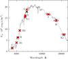 |
Fig. 1 Example SED fit for HIP 4618. The best-fitting binary model is shown with black dots, with the integrated model photometry in black crosses. The observed photometry is shown in red, with the horizontal error bar the width of the pass band. The parameters for this fit are for the giant Teff = 4750 (100) K, log g = 2.91, radius = 6.6 (0.8) R⊙ (see Table 2), and for the companion Teff = 5500 K, log g = 4.0, radius = 1.2 R⊙. |
Orbital elements of the binary companions.
4. Orbital elements
In this section we analyze the orbital properties of the 24 binary systems. We separate these systems according to their orbital period into three groups: (i) systems for which the observational time span is longer than the orbital period and for wich thus a reliable orbital solution can be derived; (ii) systems with longer orbital periods, for which it is possible to obtain a solution, but with a high level of degeneracy in the orbital parameters; and (iii) systems that present a RV trend.
4.1. Short-period binaries
Four of the 24 stars, show large RV variations (≳10 km s-1), with orbital periods P ≲ 430 days. For these, it was possible to fully constrain the orbital solution. To determine the orbital elements of the systems, we used the 2.17 version of the Systemic Console (Meschiari et al. 2009), excluding the PUCHEROS velocities, which have uncertainties up to ~100 times larger than UCLES, FEROS, and CHIRON data. The stars HIP 4618, HIP 10548, HIP 73758, and HIP 83224 have periods shorter than ~430 days. The orbital elements of the four stellar companions are listed in Table 3. Figure 2 shows the resulting RV curves. In the four cases, the RV data cover more than two orbital periods.
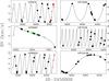 |
Fig. 2 RV variations of the six binary systems with reliable orbital solution. The black circles, blue squares, green crosses, and red triangles correspond to FEROS, CHIRON, UCLES, and PUCHEROS data, respectively. The best orbital solutions are overplotted (solid line). The post-fit RMS is typically ~10 m s-1. |
4.2. Long-period binaries
In eight cases, we observe large RV variations, but with orbital periods exceeding the observational time span. However, for HIP 59367 and HIP 104148 the phase coverage is good enough to obtain a unique orbital solution. Figure 2 shows the RV curves of these two stars. The orbital elements of the binary companions are listed in Table 3.
For the remaining six cases the orbital solution is partially degenerated because of the poor phase coverage, meaning that we can only set lower and upper limits for the orbital period and the eccentricity. Figure 3 shows the RV curve of these stars. One possible orbital solution is overplotted. In these cases it is not possible to unambiguously obtain a solution.
4.2.1. Long-period trends
The remaining 12 stars in this sample present RV variations, ranging from thousands of m s-1 level up to peak-to-peak variations of several km s-1. Half of the systems present a linear RV trend, while the remainder show some level of curvature in the observed velocities. Figure 4 shows the RV epochs of the six stars that present the smallest RV variations (~500 m s-1). Since these stars show moderate RV variations, they are candidates for hosting long-period brown dwarfs, which makes them very interesting targets for direct imaging to determine the nature of the companion. Finally, Fig. 5 shows the velocity variations of the stars that present large RV long-trend variations (≳1 km s-1), which are most likely part of a long-period stellar binary system.
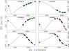 |
Fig. 3 RV variations of six long-period binaries. The black circles, blue squares, green crosses, brown open stars, and red triangles correspond to FEROS, CHIRON, UCLES, FECH, and PUCHEROS data, respectively. In each case, one possible orbital solution is overplotted (solid line). |
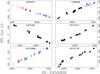 |
Fig. 4 RV variations of six long-period brown dwarf companion candidates. The black filled circles, blue squares, green crosses, brown open stars, and magenta open circles correspond to FEROS, CHIRON, UCLES, FECH, and HARPS data, respectively. |
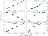 |
Fig. 5 Long-period RV trends of six binary systems. The black circles, blue squares, brown open stars, and green crosses correspond to FEROS, CHIRON, FECH, and UCLES data, respectively. |
5. Metallicity distribution
We investigated the metallicity distribution of the primary giant stars and their binary fraction. Additionally, we included 82 stars from Setiawan et al. (2004) and 150 stars from MAS08, wich makes up a sample of 395 giant stars in this analysis.
We computed the metallicities of SET04 targets using FEROS archival data. For the MAS08 targets, we used only those targets with metallicities computed by McWilliam (1990, MCW90 hereafter). We compared our sample with the MCW90 sample and we found 18 common stars. These stars are shown in Fig. 6. To remove any bias due to differences in the metallicity derived by our method and MCW90, we adjusted a linear function to correlate the two studies. We found a linear correlation of the form [Fe/H]EXP = 1.20 [Fe/H]MCW90 + 0.17. Figure 6 shows the EXPRESS versus MCW90 metallicities for the 18 targets in common. The best linear fit is overplotted. The RMS of the fit is 0.08 dex, and the Pearson linear coefficient is r = 0.90.
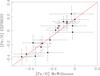 |
Fig. 6 EXPRESS versus MCW90 metallicities for the 18 targets in common. The red line corresponds to the belinear fit. |
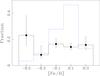 |
Fig. 7 Normalized histogram of the metallicity distribution of the primary stars (black solid line). The overall metallicity distribution of the parent sample is overplotted (dashed blue line). The width of the bins is 0.2 dex. |
Using this information, we converted from MCW90 metallicities into our metallicity scale, for all of the binaries listed in MAS08 and metallicities from MCW90. Figure 7 shows the normalized metallicity distribution of the primary stars for a total of 59 binaries, including EXPRESS, SET04, and MAS08 systems (black solid line). The error bars were computed according to Cameron (2011). The overall sample distribution is overplotted (blue dashed line). The metallicity distribution between ~−0.3 to 0.3 dex is nearly flat. Moreover, the highest fraction is obtained at metallicities around −0.5 dex. Interestingly, Raghavan et al. (2010) showed that binary systems among solar-type stars redder than B−V = 0.625 are more frequent around stars with [Fe/H] ≲−0.3 dex, in good agreement with our findings1. However, we note that the bin centered on −0.5 dex in the one with the least number of stars in the combined sample (13 systems), and therefore with the largest error bars. This result is in stark contrast with the observed metallicity distribution of planet-hosting giant stars, showing a strong increase in the giant planet frequency with increasing metallicity (e.g., Reffert et al. 2015; Jones et al. 2016), as found in solar-type stars (e.g., Fischer & Valenti 2005). This observational result also agrees with recent hydrodynamical simulations showing that the formation of binary systems across a wide range of stellar masses is not significantly affected by the metal content of the molecular clouds (Bate 2014).
Additionally, we also studied the relation in the effective temperatures (Teff) for these 18 stars in common. We compared the McWilliam and our Teff values and found a linear correlation of the form Teff(EXP) = 0.84 Teff (MCW90) + 889.1. The Pearson linear coefficient is r = 0.84. Figure 8 shows the MVW90 versus EXPRESS Teffs. The linear fit is overplotted. The error bars are not given in the MC90, and we used error bars given by the standard deviation for de Teff (MC90) values. Our values overestimate those derived by MCW90, which mainly explains why we also see a systematic difference in the derived metallicities (see Fig. 6).
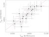 |
Fig. 8 EXPRESS versus MCW90 effective temperatures (Teff) for the 18 targets in common. The red line corresponds to the best linear fit. |
6. Period-eccentricity distribution
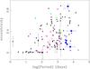 |
Fig. 9 Orbital period versus eccentricity for 130 spectroscopic giant binary stars. The red open circles represent our binaries with well-constrained orbital periods, while the blue filled circles represent those with poorly constrained orbits. The black dots, magenta filled triangles, and green filled squares correspond to MAS08, VER95, and SET04 binaries, respectively. |
We studied the period-eccentricity distribution of 130 spectroscopic binary systems in giant stars. We included all of the binaries with orbital solution from VER95, SET04, MAS08, and those presented here for which it was possible to obtain an orbital solution. Figure 9 shows the orbital period versus eccentricity of these systems. Systems with short orbital periods (P ≲ 20 days) present nearly circular orbits, similar to solar-type binaries, which is most likely explained by tidal circularization. Furthermore, there is a transition region from P ~ 20–80 days where binary systems present moderate eccentricities (e ≲ 0.4). Finally, at longer orbital periods, there is a wide spread in e, ranging from nearly circular orbits to highly eccentric systems (e ~ 0.9). This transition region and eccentricity distribution at orbital periods longer than ~100 d is also observed in solar-type binaries (e.g., Duquennoy & Mayor 1991; Jenkins et al. 2015).
The giant binary systems with moderately long orbital periods (~400–800 days) might be the precursors of the wide eccentric hot subdwarf binaries studied by Vos et al. (2015). A hot subdwarf star is a core helium-burning star located at the blue end of the horizontal branch, with colours similar to main-sequence B stars, but with much broader Balmer lines (Sargent & Searle 1968). The study of the orbital parameters of these systems will therefore be useful in binary population synthesis studies for wide sdB binaries to help determine the correct evolutionary channels of these evolved binaries.
7. Summary
We presented a sample of 24 giant stars that have revealed large radial velocity variations, which are induced by massive substellar or stellar companions. Based on precision RVs computed from high-resolution spectroscopic observations obtained as part of the EXPRESS program, we were able to fully constrain the orbital elements of 6 systems. In 6 more cases, we were able to obtain a solution although the orbital elements are poorly constrained. In the remaining cases, the primary star exhibits a RV trend, thus no solution is obtained. Six of these stars present velocity variations that are compatible with the presence of a long-period brown dwarf companion.
In addition, we studied the metallicity distribution of the primary stars. For this purpose, we retrieved literature data from two different studies, namely MAS08 and SET04. Our final sample comprised 59 spectroscopic binary systems, detected from a parent sample of 395 giant stars, covering a range of metallicities between [Fe/H] ~−0.5 and +0.5 dex. We found no significant correlation between the frequency of binary companions and the stellar metallicity. This result reinforces the fact that stellar binaries are formed mainly by gravitational collapse, which is highly insensitive to the dust content of the protostellar disk (e.g., Bate 2014), while planetary systems, including those orbiting giant stars, are formed in the protoplanetary disk by the core-accretion mechanism (e.g., Gonzalez, 1997; Santos et al. 2001; Reffert et al. 2015; Jones et al. 2016).
Finally, we studied the period-eccentricity distribution of the companions. We included a total of 130 spectroscopic binaries from the literature with known eccentricities. We found an eccentricity distribution that is characterized by short-period systems (P ≲ 20 days) that present very low eccentricities (with the exception of one case with e ~ 0.2). For orbital periods between ~20–80 days, all of the systems present moderate orbital eccentricities (e ≲ 0.4). At longer orbital periods, there is a wide spread in e, from nearly circular orbits to eccentricities as high as ~0.9. The overall distribution is qualitatively similar to the distribution observed in solar-type stars, although the circularization edge is found at slightly longer orbital periods, which is most likely explained by the stronger tidal effect induced by the larger stellar radii.
Acknowledgments
M.J. acknowledges support from FONDECYT project #3140607 and FONDEF project #CA13I10203 L. Vanzi acknowledges PUCHEROS was funded by CONICYT through projects FONDECYT No. 1095187 and No. 1130849. H. Drass acknowledges financial support from FONDECYT project #3150314 R.E.M. acknowledges support by VRID-Enlace 214.016.001-1.0 and the BASAL Centro de Astrofísica y Tecnologías Afines (CATA) PFB–06/2007. F.O.E. acknowledges support from FONDECYT through postdoctoral grant 3140326 and from project IC120009 “Millennium Institute of Astrophysics (MAS)” of the Iniciativa Científica Milenio del Ministerio de Economía, Fomento y Turismo de Chile.
References
- Alonso, A., Arribas, S., Benz, W., & Martínez-Roger, C. 1999, A&A, 140, 261 [Google Scholar]
- Arenou, F., Grenon, M., & Gómez, A. 1992, A&A, 258, 104 [NASA ADS] [Google Scholar]
- Baranne, A., Queloz, D., Mayor, M., et al. 1996, A&A, 119, 373 [Google Scholar]
- Bate, M. R. 2014, MNRAS, 442, 285 [NASA ADS] [CrossRef] [Google Scholar]
- Butler, R. P., Marcy, G. W., Williams, E., et al. 1996, PASP, 108, 500 [NASA ADS] [CrossRef] [Google Scholar]
- Cameron, E. 2011, PASA, 28, 128 [NASA ADS] [CrossRef] [Google Scholar]
- Degroote, P., Acke, B., Samadi, R., et al., 2011, A&A, 536, A82 [NASA ADS] [CrossRef] [EDP Sciences] [Google Scholar]
- Diego, F., Charalambous, A., Fish, A. C., & Walker, D. D. 1990, Proc. Soc.Photo-Opt. Instr. Eng., 1235, 562 [Google Scholar]
- Duquennoy, A., & Mayor, M. 1991, A&A, 248, 485 [NASA ADS] [Google Scholar]
- Endl, M., Kurster, M., & Els, S. 2000, A&A, 362, 585 [Google Scholar]
- Fischer, D. A., & Valenti, J. 2005, ApJ, 622, 1102 [NASA ADS] [CrossRef] [Google Scholar]
- Gonzalez, G. 1997, MNRAS, 285, 403 [NASA ADS] [CrossRef] [Google Scholar]
- Jenkins, J. S., Díaz, M., Jones, H. R. A., et al. 2015, MNRAS, 453, 1439 [NASA ADS] [CrossRef] [Google Scholar]
- Jones, M. I., Jenkins, J. S., Rojo, P., & Melo, C. H. F. 2011, A&A, 536, A71 [NASA ADS] [CrossRef] [EDP Sciences] [Google Scholar]
- Jones, M. I., Jenkins, J. S., Rojo, P., Melo, C. H. F., Bluhm, P., 2013, A&A, 556, A78 [NASA ADS] [CrossRef] [EDP Sciences] [Google Scholar]
- Jones, M. I., Jenkins, J. S., Rojo, P., et al. 2015, A&A, 580, A14 [NASA ADS] [CrossRef] [EDP Sciences] [Google Scholar]
- Jones, M.I., Jenkins, J.S, Brahm, R., et al. 2016, A&A, 590, A38 [NASA ADS] [CrossRef] [EDP Sciences] [Google Scholar]
- Kaufer, A., Stahl, O., Tubbesing, S., et al. 1999, The Messenger, 95, 8 [Google Scholar]
- Kurucz, R.L., 1979, ApJ, 40, 1 [Google Scholar]
- Kurucz, R. L., 1993, ATLAS9 Stellar Atmosphere Programs and 2 km s-1 Grid, CD-ROM No. 13 (Cambridge, Smithsonian Astrophysical Observatory) [Google Scholar]
- Lada, C. J. 2006, ApJ, 640, L63 [NASA ADS] [CrossRef] [Google Scholar]
- Machida, M. N. 2008, ApJ, 682, 1 [NASA ADS] [CrossRef] [Google Scholar]
- Massarotti, A., Latham, D., Stefanik, R. P., & Fogel, J. 2008, AJ, 135, 209 [NASA ADS] [CrossRef] [Google Scholar]
- Mayor, M., Pepe, F., Queloz, D., et al. 2003, The Messenger, 114, 20 [NASA ADS] [Google Scholar]
- McWilliam, A. 1990, ApJS, 74, 1075 [NASA ADS] [CrossRef] [Google Scholar]
- Meschiari, S., Wolf, A. S., Rivera, E., et al. 2009, PASJ, 121, 1016 [Google Scholar]
- Pan, K., Tan, H., Duan, C., & Shan, H. 1998, ASP Conf., 138, 267 [Google Scholar]
- Perryman, M. A. C., Lindegren, L., Kovalevsky, J., et al. 1997, A&A, 343, L49 [NASA ADS] [Google Scholar]
- Raghavan, D., McAlister, H. A., Henry, T. J., et al. 2010, ApJ, 190, 1 [NASA ADS] [Google Scholar]
- Reffert, S., Bergmann, C., Quirrenbach, A., et al. 2015, A&A, 574, A116 [NASA ADS] [CrossRef] [EDP Sciences] [Google Scholar]
- Salasnich, L., Girardi, L., Weiss, A., & Chiosi, C. 2000, A&A, 361, 1023 [NASA ADS] [Google Scholar]
- Santos, N. C., Israelian, G., & Mayor, M. 2001, A&A, 373, 1019 [NASA ADS] [CrossRef] [EDP Sciences] [Google Scholar]
- Sargent, W. L. W., & Searle, L. 1968, ApJ, 152, 443 [NASA ADS] [CrossRef] [Google Scholar]
- Sato, B., Izumiura, H., Toyota, E., et al. 2008, PASJ, 60, 539 [NASA ADS] [Google Scholar]
- Setiawan, J., Pasquini, L., & da Silva, L. 2004, A&A, 421, 241 [NASA ADS] [CrossRef] [EDP Sciences] [Google Scholar]
- Sneden, C. 1973, ApJ, 184, 839 [NASA ADS] [CrossRef] [Google Scholar]
- Tassoul, J. L. 1987, ApJ, 322, 856 [NASA ADS] [CrossRef] [Google Scholar]
- Tassoul, J. L. 1988, ApJ, 324, 71 [Google Scholar]
- Tassoul, J. L. 1992, ApJ, 395, 259 [NASA ADS] [CrossRef] [Google Scholar]
- Tokovinin, A., Fisher, D., Bonati, M. et al. 2013, PASP, 125, 1336 [NASA ADS] [CrossRef] [Google Scholar]
- Tonry, J., & Davis, M., 1979, AJ, 84, 1511 [NASA ADS] [CrossRef] [Google Scholar]
- Vanzi, L., Chacon, J., Helminiak, K.G., et al. 2012, MNRAS, 424, 2770 [NASA ADS] [CrossRef] [Google Scholar]
- Verbunt, F., & Phinney, E. S. 1995, A&A, 296, 709 [NASA ADS] [Google Scholar]
- Villaver, E., & Livio, M. 2009, ApJ, 705, 81 [Google Scholar]
- Vos, J., Østensen, R. H., Degroote, P., et al. 2012, A&A, 548, A6 [NASA ADS] [CrossRef] [EDP Sciences] [Google Scholar]
- Vos, J., Østensen, R. H., Németh, P., et al. 2013, A&A, 559, A54 [NASA ADS] [CrossRef] [EDP Sciences] [Google Scholar]
- Vos, J., Østensen, R. H., Marchant, P., et al. 2015, A&A, 579, A49 [NASA ADS] [CrossRef] [EDP Sciences] [Google Scholar]
- Wittenmyer, R. A., Endl, M., Wang, L., et al. 2011, ApJ, 743, 184 [NASA ADS] [CrossRef] [Google Scholar]
- Wittenmyer, R. A., Butler, R. P., Wang, L., et al. 2016, MRAS, 455, 138 [Google Scholar]
- Zahn, J. P. 1977, A&A, 57, 383 [NASA ADS] [Google Scholar]
- Zahn, J. P., & Bouchet, L. 1989, A&A, 210, 112 [NASA ADS] [Google Scholar]
Appendix A: Radial velocity tables
Radial velocity variations for HIP 4618.
Radial velocity variations for HIP 7118.
Radial velocity 10548.
Radial velocity variations for HIP 22479.
Radial velocity variations for HIP 59016.
Radial velocity variations for HIP 59367.
Radial velocity variations for HIP 64647.
Radial velocity variations for HIP 64803.
Continued table for HIP 64803.
Radial velocity variations for HIP 66924.
Radial velocity variations for HIP 67890.
Radial velocity variations for HIP 68099.
Radial velocity variations for HIP 71778.
Radial velocity variations for HIP 73758.
Radial velocity variations for HIP 74188.
Radial velocity variations for HIP 75331.
Radial velocity variations for HIP 76532.
Radial velocity variations for HIP 76569.
Radial velocity variations for HIP 77888.
Radial velocity variations for HIP 83224.
Radial velocity variations for HIP 101911.
Radial velocity variations for HIP 103836.
Radial velocity variations for HIP 104148.
Radial velocity variations for HIP 106055.
Radial velocity variations for HIP 107122.
Appendix B: Atmospheric parameters
Atmospheric parameters for Setiawan data.
All Tables
All Figures
|
Fig. 1 Example SED fit for HIP 4618. The best-fitting binary model is shown with black dots, with the integrated model photometry in black crosses. The observed photometry is shown in red, with the horizontal error bar the width of the pass band. The parameters for this fit are for the giant Teff = 4750 (100) K, log g = 2.91, radius = 6.6 (0.8) R⊙ (see Table 2), and for the companion Teff = 5500 K, log g = 4.0, radius = 1.2 R⊙. |
| In the text | |
|
Fig. 2 RV variations of the six binary systems with reliable orbital solution. The black circles, blue squares, green crosses, and red triangles correspond to FEROS, CHIRON, UCLES, and PUCHEROS data, respectively. The best orbital solutions are overplotted (solid line). The post-fit RMS is typically ~10 m s-1. |
| In the text | |
|
Fig. 3 RV variations of six long-period binaries. The black circles, blue squares, green crosses, brown open stars, and red triangles correspond to FEROS, CHIRON, UCLES, FECH, and PUCHEROS data, respectively. In each case, one possible orbital solution is overplotted (solid line). |
| In the text | |
|
Fig. 4 RV variations of six long-period brown dwarf companion candidates. The black filled circles, blue squares, green crosses, brown open stars, and magenta open circles correspond to FEROS, CHIRON, UCLES, FECH, and HARPS data, respectively. |
| In the text | |
|
Fig. 5 Long-period RV trends of six binary systems. The black circles, blue squares, brown open stars, and green crosses correspond to FEROS, CHIRON, FECH, and UCLES data, respectively. |
| In the text | |
|
Fig. 6 EXPRESS versus MCW90 metallicities for the 18 targets in common. The red line corresponds to the belinear fit. |
| In the text | |
|
Fig. 7 Normalized histogram of the metallicity distribution of the primary stars (black solid line). The overall metallicity distribution of the parent sample is overplotted (dashed blue line). The width of the bins is 0.2 dex. |
| In the text | |
|
Fig. 8 EXPRESS versus MCW90 effective temperatures (Teff) for the 18 targets in common. The red line corresponds to the best linear fit. |
| In the text | |
|
Fig. 9 Orbital period versus eccentricity for 130 spectroscopic giant binary stars. The red open circles represent our binaries with well-constrained orbital periods, while the blue filled circles represent those with poorly constrained orbits. The black dots, magenta filled triangles, and green filled squares correspond to MAS08, VER95, and SET04 binaries, respectively. |
| In the text | |
Current usage metrics show cumulative count of Article Views (full-text article views including HTML views, PDF and ePub downloads, according to the available data) and Abstracts Views on Vision4Press platform.
Data correspond to usage on the plateform after 2015. The current usage metrics is available 48-96 hours after online publication and is updated daily on week days.
Initial download of the metrics may take a while.