| Issue |
A&A
Volume 593, September 2016
|
|
|---|---|---|
| Article Number | A15 | |
| Number of page(s) | 4 | |
| Section | Numerical methods and codes | |
| DOI | https://doi.org/10.1051/0004-6361/201628143 | |
| Published online | 29 August 2016 | |
Research Note
Optimal cosmic microwave background map-making in the presence of cross-correlated noise
1 Dipartimento di Fisica, Università di Roma “Tor Vergata”, via della Ricerca Scientifica 1, 00133 Roma, Italy
e-mail: giancarlo.degasperis@roma2.infn.it
2 Sezione INFN Roma 2, via della Ricerca Scientifica 1, 00133 Roma, Italy
3 Dipartimento di Fisica, Sapienza Università di Roma, piazzale Aldo Moro 5, 00185 Roma, Italy
4 Sezione INFN Roma 1, piazzale Aldo Moro 5, 00185 Roma, Italy
Received: 16 January 2016
Accepted: 12 July 2016
Aims. We present an extension of the ROMA map-making algorithm for the generation of optimal cosmic microwave background polarization maps. The new code allows for a possible cross-correlated noise component among the detectors of a CMB experiment. A promising application is the forthcoming LSPE balloon-borne experiment, which is devoted to the accurate observation of CMB polarization at large angular scales.
Methods. We generalized the noise covariance matrix in time domain to account for all the off-diagonal terms due to the detector cross-talk. Hence, we performed preliminary forecasts of the LSPE-SWIPE instrument.
Results. We found that considering the noise cross-correlation among the detectors results in a more realistic estimate of the angular power spectra. In particular, the extended ROMA algorithm has provided a considerable reduction of the spectra error bars. We expect that this improvement could be crucial in constraining the B-mode polarization at the largest scales.
Key words: cosmic background radiation / methods: data analysis
© ESO, 2016
1. Introduction
The temperature and polarization patterns of cosmic microwave background (CMB) have been an invaluable source of cosmological information. While polarization E-modes have been widely observed and analyzed (e.g., Planck: Planck Collaboration XI 2016), B-modes are still buried into foreground signal and experimental noise (e.g., BICEP2/Keck and Planck Collaborations et al. 2015). Nowadays, the hunting for B-modes represents one of the most relevant and exciting research fields in cosmology. In fact, a B-mode detection in CMB polarization would provide a definitive confirmation of the existence of a gravitational waves primordial background, as expected in the inflation paradigm (Lyth & Riotto 1999).
Because of the low signal-to-noise ratio, polarization observations require large multidetector arrays. The increased detector array size and the integration of many pixels on the same wafer rise the problem of cross talk among the detectors. This can be due to either focal plane temperature variations and/or atmospheric fluctuations. Both these effects are expected to produce common-mode noise in the detectors. This noise cross-correlation has to be properly taken into account in the map-making procedure.
After the pioneering work of Wright (1996), map-making has been thoroughly studied in the literature (see e.g., Cantalupo et al. 2010, and references therein). However, cross-correlated noise among the detectors has not been discussed as much and is crudely neglected. The only detailed treatment that allows us to take common-mode noise into account explicitly and properly is that by Patanchon et al. (2008), for intensity measurements only. Given the pressing interest on primordial B-mode detection, a specific treatment of noise cross-correlation in polarization measurements is now necessary.
Among the next generation of CMB experiments, we focus on the Large-Scale Polarization Explorer1 (LSPE) balloon mission, which is devoted to accurate observations of CMB polarization at large angular scales (see e.g., de Bernardis et al. 2012). The LSPE is expected to improve the limit on the ratio of tensor-to-scalar perturbation amplitudes down to r ≲ 0.03.
In this work we present an extension of the ROMA map-making code (Roma optimal map-making algorithm, de Gasperis et al. 2005) to produce optimal CMB polarization maps out of cross-correlated multi-detector CMB observations. In particular, we discuss how a proper inclusion of the detector noise cross-correlations results in more realistic estimates of the angular power spectra error bars. This benefit could be crucial for the detection of a primordial B-mode signal at low multipoles.
2. Formalism, algebra, and noise model
A CMB experiment observes the sky at a given resolution (i.e. with Np pixels in the sky) and collects Nd samples in a given temporal sequence, the time ordered data (TOD). Once the data are calibrated, any artifact is flagged out and the pointing is reconstructed, the first step in the CMB data analysis is the estimation of optimal sky maps from the TOD. In the literature two main strategies are present: a maximum-likelihood (minimum-variance) approach (see e.g., de Gasperis et al. 2005, and references therein) and destriping techniques (see e.g., Tristram et al. 2011, and references therein).
We take the cross-correlated noise component among detectors into account in the following way. The observational data from one detector can be modeled as  (1)Here, D is the TOD, A is the generalized pointing matrix, S = (I,Q,U) is the map triplet and n is the instrumental noise, which accounts for any systematic effects, cosmic ray hits, etc. When dealing with multiple detector observations, the TODs from individual detectors are simply concatenated end-to-end. Under the assumption of a Gaussian and stationary noise, the generalized least squared approach yields the following maximum-likelihood estimator for the signal
  (2)The noise covariance matrix in the time domain, N ≡ ⟨ntnt′⟩, is block diagonal only in the case of no cross-correlation among samples of different detectors. The present version of the ROMA algorithm takes into account all the off-diagonal terms, which have usually been neglected in past works. The solution of Eq. (2) is a very computationally demanding task because of the large size of the matrix N, kNp × kNp, where k is the number of detectors. Our algorithm adopts a Fourier-based, preconditioned conjugate-gradient iterative method.
The choice of the noise model is clearly a crucial issue. In general, the detector noise spectrum is in the sum of a stationary Gaussian white noise at higher frequencies and a 1 /f component at lower frequencies, which implies an unavoidable correlation among different samples in the single detector time stream. A further complication is the presence of the noise common-mode seen by all the detectors. Its contribution has been estimated directly from data (see e.g., Masi et al. 2006). The cross-correlated noise is typical of ground- and balloon-based experiment, as it is sourced mainly by atmospheric fluctuations. However, it could also affect space missions, due to common-mode detector temperature drifts. This work is addressed to the balloon regime, but our treatment is completely general.
3. Forecasts of the LSPE-SWIPE experiment
In this work we focus on the forthcoming LSPE balloon-borne experiment that is devoted to the accurate measurement of CMB polarization at large angular scales.
We use the level of noise cross-correlation among the CMB polarimeters estimated for BOOMERanG (Masi et al. 2006) as a benchmark for our simulations. Since the deep similarities between BOOMERanG and the LSPE-SWIPE experiment (long duration stratospheric bolometric experiments subject to atmospheric common-mode fluctuations), we found it natural to use the BOOMERanG noise properties for the LSPE-SWIPE preliminary forecasts.
3.1. The instrument
During its circumpolar Arctic flight, LSPE will scan the sky by spinning around the local vertical, while keeping the telescope elevation constant for long periods, in the range 30 to 55 deg. The azimuth scan speed will be set around 2 rpm, i.e. 12 deg s-1. A large portion of the northern sky (around 25% of the celestial sphere) is expected to be observed with an angular resolution of about 1.5 degrees FWHM.
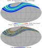 |
Fig. 1 Sky region scanned by 18 sample detectors, sparsely located in the two focal planes of LSPE-SWIPE, in ecliptic coordinates (upper panel) and the inverse pixel condition number Rcond as an estimator of polarization angle coverage per pixel (lower panel). In our definition, Rcond = 1/2 in case of perfect angle coverage uniformity. Both maps are at HEALPix (see Górski et al. 2005) Nside = 128. |
The payload will host two instruments: the Short Wavelength Instrument for the Polarization Explorer (SWIPE; de Bernardis et al. 2012), which will map the sky in three frequency bands centered at 140, 220, and 240 GHz; and the STRatospheric Italian Polarimeter (STRIP, Bersanelli et al. 2012), which will survey the same sky region in two frequency bands centered at 43 and 90 GHz.
In this work we focus on the SWIPE bolometric polarimeter instrument, which is characterized by two symmetric orthogonally-placed focal planes hosting an overall number of 110 detectors per frequency. The peculiarity of SWIPE will be the presence of a half wave plate (HWP) polarization modulator as first optical element, followed by a 50 cm aperture refractive telescope, a beam-splitting polarizer, and finally the multimoded focal planes. The SWIPE detectors are multimode spiderweb TES bolometers operating at 0.3 K (see Gualtieri et al. 2016).
In Fig. 1 we show the sky region as seen by a subset of 18 LSPE-SWIPE detectors, which are arranged in three triples sparsely located in each of the two focal planes, and the corresponding angle coverage estimator, for one observation day. The maps are at HEALPix2 resolution Nside = 128 (27.5′ per pixel, see Górski et al. 2005). In Fig. 2 we show the temperature and polarization intensity power as a function of frequency for one bolometer of the SWIPE instrument, assuming the nominal HWP steps of 11.25 °/min.
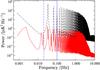 |
Fig. 2 Power vs. frequency for temperature (in dashed black line) and polarization intensity (in solid red line) in the case of half wave plate (HWP) steps of 11.25 °/min. In our simulations, we focused on two noise knee frequencies: 0.02 and 0.1 Hz. |
Because of the large number of detectors we expect that the noise cross-correlation may represent a critical issue and therefore, a proper treatment is necessary. However, we highlight that the cross-correlation among the detectors must be accounted for in relation to the possible filtering of the data; the benefit of considering the noise common mode crucially depends on the magnitude of the low-frequency cut. For instance, we tested the extended ROMA code on the BOOMERanG real data set and we found no remarkable benefits with respect to the past analysis that completely neglected the noise cross-correlation. The low impact of the new treatment is due to the heavy filter of low-frequency data streams performed on the real data set, which has crudely cut out the information at large angular scales where the cross-correlated noise effect is more relevant. However, using simulated unfiltered data we found that a proper treatment of the noise cross-correlation results in considerably better maps and angular power spectrum estimates (the spectrum standard deviations have been reduced up to 20%; see Buzzelli 2015; and Buzzelli et al. 2016). In the following simulations, we first assume that no filter was applied on the data, hence we face a specific case where reasonable frequency cuts have been performed.
3.2. Simulations
We generate simulated TOD based on the SWIPE scanning strategy and polarimeter angles for one day of observations (Nd = 8.64 × 10⁶ samples per detector) and telescope elevation of 45 deg. In particular we choose an HWP stepping of 11.25 °/min, repeatedly scanning the range 0 ◦ – 78.75 ◦, and we consider 18 detectors as described above.
We assume the cosmological parameters estimated by Planck (Planck Collaboration XIII 2016) with a tensor-to-scalar ratio r = 0.09. The noise is simulated assuming the bolometer to be photon-noise limited with a white plateau of 15 μKCMB at higher frequencies and a 1 /fα noise with α = 2 at lower frequencies, as expected for the multimoded 140 GHz channel. We focus on two knee frequencies, 0.02 and 0.1 Hz, the expected best and worst case. For each knee frequency, we consider two different common-mode configurations:
-
1.
The cross-correlation is present in both the 1 /f2 and white noise part of the spectrum. In the former, the cross-correlated component is shared by all the detectors; in the latter we assume 10% of cross-correlation among each triple and 1% among any other detector, with respect to the auto noise spectrum. This situation is the analog to that found in the BOOMERanG analysis;
-
2.
the cross-correlation is limited to the 1 /f2 part of the noise spectrum with no white noise common mode.
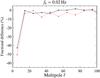 |
Fig. 3 Fractional difference of the BB power spectra error bars from LSPE-SWIPE simulations estimated considering and neglecting the bolometer noise cross-correlation of case 1 (in dashed red line) and case 2 (in solid black line) for a knee frequency fk =0.02 Hz. |
In the four cases, we produced 50 signal-only, noise-only, and signal plus noise Monte Carlo simulated maps, both taking into account or not the noise cross-correlation among detectors in the map-making code. Then, we applied the MASTER power spectrum estimator (Hivon et al. 2002) to the maps.
It should be taken into account that, at large angular scales, the MASTER spectrum estimator method may not be the most convenient choice. As mentioned by Molinari et al. (2014), at low multipoles a quadratic maximum likelihood estimator (QML) is preferable. Nonetheless, the aim of this work is to check the reliability of an improved map-making code, which can also be successfully tested by using quicker but less accurate angular power spectra estimates.
In Fig. 3 we show the fractional difference of BB power spectra error bars estimated considering and neglecting the noise cross-correlation in the algorithm, assuming the data set to be contaminated by the two noise configuration described above, for a knee frequency fk =0.02 Hz. The results for fk =0.1 Hz are shown in Fig. 4. It is evident that neglecting the cross-correlation affects heavily the power spectra error bars. For a knee frequency fk =0.02 Hz, the inclusion of the cross-correlation has the effect of reducing the spectra error bars up to 40−50%. For fk =0.1 Hz, we find an improvement up to 50−60%.
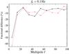 |
Fig. 4 Fractional difference of the BB power spectra error bars from LSPE-SWIPE simulations estimated considering and neglecting the bolometer noise cross-correlation of case 1 (in dashed red line) and case 2 (in solid black line) for a knee frequency fk =0.1 Hz. |
3.3. Comparison with filtering techniques
As mentioned above, to reduce the low-frequency noise contribution, it is a common choice to high pass the data stream at some cut frequency fc. However, this method is not lossless, as part of the signal information is filtered out as well.
While this option appears to be feasible when the low-frequency cutoff fc is 0.02 Hz since the cosmological signal at lower frequencies is negligible, we found that (see Fig. 2) if fc = 0.05 or 0.1 Hz the high-pass filter will cut the polarization intensity power of ≃ 17 and 25% and the I Stokes power of ≃ 31 and 48%, respectively.
To estimate the effect of data filtering on the power spectra error bars, we perform a similar analysis as above but with high-pass frequencies fc = 0.02,0.05 and 0.1 Hz and neglecting the cross-correlated noise in the analysis for the noise configuration of case 2 and fk =0.1 Hz.
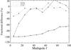 |
Fig. 5 Fractional difference between the BB power spectrum error bars estimated including the noise cross-correlation and applying a low-frequency data filtering (neglecting the cross-correlated noise) at fc =0.02 Hz in dotted line, fc =0.05 Hz in dashed line and fc =0.1 Hz in solid line. The BB spectra correspond to the noise configuration of case 2 with fk =0.1 Hz. |
We compare these results with the power spectra error bars estimated accounting for cross-correlated noise with no data filtering. In Fig. 5 we show the fractional difference of the error bars between the cases with cross-correlation and low-frequency filtering. It can be noticed that, by including the noise cross-correlation in the map-making code, we are recovering smaller BB power spectrum error bars compared to the case with data filtering. At very low multipoles, the improvement is up to 30% and 100% for the fc =0.02 Hz and fc ≥0.05 Hz cases, respectively.
It is not the aim of this work to forecast a suitable filtering strategy for LSPE-SWIPE in relation to the inclusion of the noise cross-correlation in the analysis. This would require a more
accurate specifications of many parameters, such as telescope elevation, azimuth scan velocity and HWP velocity. However, we stress that the improvements provided by the extended ROMA code may result in a less dramatic filtering of low-frequency data, thus preserving most of the cosmological information.
4. Conclusions
We presented a new version of the ROMA map-making code extended to a possible cross-correlated noise component among the detectors of a CMB experiment.
This effect must be properly taken into account in the data analysis of any experiment aimed at detection of B-mode polarization, either from space, balloons or ground.
Among the next generation of CMB experiments, we focus on the forthcoming LSPE balloon-borne experiment, devoted to the accurate observation of CMB polarization at large angular scales with the primary aim to constrain the primordial B-mode polarization.
We applied the extended ROMA algorithm to simulated data of the LSPE-SWIPE instrument and found that the inclusion of cross-correlation provides spectra error bars smaller up to 50−60%, depending on the chosen knee frequency. We point out that this improvement could be crucial in constraining the B-mode polarization.
A very relevant issue is to compare these results with a possible low-frequency data filtering, commonly used for ground-based and balloon-borne experiments. We found that accounting for cross-correlated noise with no filtering is a viable option, which is certainly less crude than a cut of low-frequency streams, with the additional potential advantage of not removing cosmological information at the largest scales.
Acknowledgments
We acknowledge the use of the HEALPix package (Górski et al. 2005) and of the FFTW library (Frigo & Johnson 2005). We wish to thank Silvia Masi and Marina Migliaccio for useful suggestions and discussions, and LSPE collaboration for providing us with the LSPE-SWIPE pointing informations.
References
- Bersanelli, M., Mennella, A., Morgante, G., et al. 2012, in SPIE Conf. Ser., 8446, 7 [Google Scholar]
- BICEP2/Keck and Planck Collaborations 2015, Phys. Rev. Lett., 114, 101301 [NASA ADS] [CrossRef] [PubMed] [Google Scholar]
- Buzzelli, A. 2015, Master’s Thesis, Università di Roma Tor Vergata, Italy [Google Scholar]
- Buzzelli, A., Cabella, P., de Gasperis, G., & Vittorio, N. 2016, J. Phys. Conf. Ser., 689, 012003 [NASA ADS] [CrossRef] [Google Scholar]
- Cantalupo, C. M., Borrill, J. D., Jaffe, A. H., Kisner, T. S., & Stompor, R. 2010, ApJS, 187, 212 [NASA ADS] [CrossRef] [Google Scholar]
- de Bernardis, P., Aiola, S., Amico, G., et al. 2012, in SPIE Conf. Ser., 8452, 3 [Google Scholar]
- de Gasperis, G., Balbi, A., Cabella, P., Natoli, P., & Vittorio, N. 2005, A&A, 436, 1159 [NASA ADS] [CrossRef] [EDP Sciences] [Google Scholar]
- Frigo, M., & Johnson, S. G. 2005, Proceedings of the IEEE, 93, 216, special issue on Program Generation, Optimization, and Platform Adaptation [Google Scholar]
- Górski, K. M., Hivon, E., Banday, A. J., et al. 2005, ApJ, 622, 759 [NASA ADS] [CrossRef] [Google Scholar]
- Gualtieri, R., Battistelli, E. S., Cruciani, A., et al. 2016, J. Low Temp. Phys., 184, 527 [Google Scholar]
- Hivon, E., Górski, K. M., Netterfield, C. B., et al. 2002, ApJ, 567, 2 [NASA ADS] [CrossRef] [Google Scholar]
- Lyth, D. H. D. H., & Riotto, A. A. 1999, Phys. Rep., 314, 1 [Google Scholar]
- Masi, S., Ade, P. A. R., Bock, J. J., et al. 2006, A&A, 458, 687 [NASA ADS] [CrossRef] [EDP Sciences] [Google Scholar]
- Molinari, D., Gruppuso, A., Polenta, G., et al. 2014, MNRAS, 440, 957 [NASA ADS] [CrossRef] [Google Scholar]
- Patanchon, G., Ade, P. A. R., Bock, J. J., et al. 2008, ApJ, 681, 708 [NASA ADS] [CrossRef] [Google Scholar]
- Planck Collaboration XI. 2016, A&A, in press, DOI: 10.1051/0004-6361/201526926 [Google Scholar]
- Planck Collaboration XIII. 2016, A&A, in press, DOI: 10.1051/0004-6361/201525830 [Google Scholar]
- Tristram, M., Filliard, C., Perdereau, O., et al. 2011, A&A, 534, A88 [NASA ADS] [CrossRef] [EDP Sciences] [Google Scholar]
- Wright, E. L. 1996, ArXiv e-prints [arXiv:astro-ph/9612006] [Google Scholar]
All Figures
|
Fig. 1 Sky region scanned by 18 sample detectors, sparsely located in the two focal planes of LSPE-SWIPE, in ecliptic coordinates (upper panel) and the inverse pixel condition number Rcond as an estimator of polarization angle coverage per pixel (lower panel). In our definition, Rcond = 1/2 in case of perfect angle coverage uniformity. Both maps are at HEALPix (see Górski et al. 2005) Nside = 128. |
| In the text | |
|
Fig. 2 Power vs. frequency for temperature (in dashed black line) and polarization intensity (in solid red line) in the case of half wave plate (HWP) steps of 11.25 °/min. In our simulations, we focused on two noise knee frequencies: 0.02 and 0.1 Hz. |
| In the text | |
|
Fig. 3 Fractional difference of the BB power spectra error bars from LSPE-SWIPE simulations estimated considering and neglecting the bolometer noise cross-correlation of case 1 (in dashed red line) and case 2 (in solid black line) for a knee frequency fk =0.02 Hz. |
| In the text | |
|
Fig. 4 Fractional difference of the BB power spectra error bars from LSPE-SWIPE simulations estimated considering and neglecting the bolometer noise cross-correlation of case 1 (in dashed red line) and case 2 (in solid black line) for a knee frequency fk =0.1 Hz. |
| In the text | |
|
Fig. 5 Fractional difference between the BB power spectrum error bars estimated including the noise cross-correlation and applying a low-frequency data filtering (neglecting the cross-correlated noise) at fc =0.02 Hz in dotted line, fc =0.05 Hz in dashed line and fc =0.1 Hz in solid line. The BB spectra correspond to the noise configuration of case 2 with fk =0.1 Hz. |
| In the text | |
Current usage metrics show cumulative count of Article Views (full-text article views including HTML views, PDF and ePub downloads, according to the available data) and Abstracts Views on Vision4Press platform.
Data correspond to usage on the plateform after 2015. The current usage metrics is available 48-96 hours after online publication and is updated daily on week days.
Initial download of the metrics may take a while.