© ESO, 2016

1. Introduction

Luminosity functions (LF) are fundamental properties of the observed galaxy populations that provide important constraints on models of galaxy formation and evolution (e.g. Lacey et al. 2015; Schaye et al. 2015). Studying the LF at far-infrared (FIR) and sub-millimetre (sub-mm) wavelengths is critical. Half of the energy ever emitted by galaxies has been absorbed by dust and re-radiated in the FIR and sub-mm (Hauser & Dwek 2001; Dole et al. 2006). The spectra of most IR luminous galaxies peak in the FIR and sub-mm (Symeonidis et al. 2013; Casey et al. 2014). Finally, our knowledge of the FIR and sub-mm LF is relatively poor.

The first 250 μm LF measurement was made by Eales et al. (2009) with observations conducted using the Balloon-borne Large Aperture Submm Telescope (BLAST; Devlin et al. 2009). Herschel (Pilbratt et al. 2010) significantly improved over BLAST with increased sensitivity, higher resolution, and larger areal coverage. Dye et al. (2010) detected strong evolution in the 250 μm LF out to z ~ 0.5, using the Herschel-Astrophysical Terahertz Large Area Survey (H-ATLAS; Eales et al. 2010a,b). Using the Herschel Multi-tiered Extragalactic Survey (HerMES; Oliver et al. 2012), Vaccari et al. (2010) presented the first constraints on the 250, 350, and 500 μm as well as the infrared bolometric (8−1000 μm) LF at z< 0.2. More recently, combining Herschel data with multi-wavelength datasets, Marchetti et al. (2016) derived the LF at 250, 350, and 500 μm as well as the bolometric LF over 0.02 <z< 0.5. Evolution in luminosity (${\mathit{L}}_{\mathrm{250}}^{\mathrm{\ast }}\mathrm{\propto }\mathrm{(}\mathrm{1}\mathrm{+}\mathit{z}{\mathrm{)}}^{\mathrm{5.3}\hspace{0.17em}\mathrm{\pm }\hspace{0.17em}\mathrm{0.2}}$) and density (${\mathrm{\Phi }}_{\mathrm{250}}^{\mathrm{\ast }}\mathrm{\propto }\mathrm{(}\mathrm{1}\mathrm{+}\mathit{z}{\mathrm{)}}^{\mathrm{-}\mathrm{0.6}\hspace{0.17em}\mathrm{\pm }\hspace{0.17em}\mathrm{0.4}}$) are found at z< 0.2. Marchetti et al. (2016), however, were unable to constrain evolution beyond z ~ 0.2, as only the brightest galaxies can be individually detected at higher redshifts. Despite the significant progress made, the determination of the LF is still hampered by many difficulties. Large samples over large areas are required for accuracy. We need to focus on smaller areas with increased sensitivity, however, to probe the faint end. At the Herschel-SPIRE (Griffin et al. 2010) wavelengths, confusion (related to the relatively poor angular resolution) is a serious challenge for source extraction, flux estimation, and cross-identification with sources detected at other wavelengths. In addition, issues such as completeness and selection effects due to the combination of several surveys are extremely difficult to quantify (e.g. Casey et al. 2012).

In this paper, we present a new analysis of the 250 μm LF by stacking deep optically selected galaxy catalogues from the Sloan Digital Sky Survey (SDSS) on the SPIRE 250 μm images. We bypass some major difficulties in previous measurements (e.g. complicated selection effects, reliability of the cross-identification). The paper is organised as follows. In Sect. 2, we describe the relevant data products from the SDSS and Herschel surveys. In Sect. 3, we explain our stacking method, which recovers the mean properties and underlying distribution functions. In Sect. 4, we present our results and compare with previous measurements. Finally, we give conclusions in Sect. 5. We assume Ω_m = 0.25, Ω_Λ = 0.75, and H₀ = 73 km s^-1 Mpc^-1. Flux densities are corrected for Galactic extinction (Schlegel et al. 1998).

2. Data

2.1. Optical galaxy samples from SDSS

The SDSS Data Release 12 (DR 12) contains observations from 1998 to 2014 over a third of the sky (Alam et al. 2015) in ugriz. The DR 12 includes photometric redshift (z_phot) using an empirical method known as a kd-tree nearest neighbour fit (KF) (Csabai et al. 2007), which is extended with a template-fitting method to derive parameters, such as k corrections and absolute magnitudes, using spectral templates from Dobos et al. (2012). The DR 12 features an expanded training set (extending to z = 0.8), an updated method of template-fitting, and a more detailed approach to errors (Beck et al. 2016). Following recommendations on the SDSS website, we selected galaxies (located in the three Galaxy And Mass Assembly (GAMA) equatorial fields with Herschel coverage) with photoErrorClass equal to 1, −1, 2, and 3, which have an average RMS error in (1 + z) of 0.02, 0.03, 0.03 and 0.03, respectively. We constructed volume-limited samples in five redshift bins, z1 = [0.02,0.1], z2 = [0.1,0.2], z3 = [0.2,0.3], z4 = [0.3,0.4] and z5 = [0.4,0.5]. In each bin, we only selected galaxies that were bright enough to be seen throughout the corresponding volume, given the apparent magnitude limit is r = 20.4 which corresponds to the 90% completeness limit for single pass images (Annis et al. 2014). We also take the most adverse k correction in a given redshift bin into account in deriving the luminosity limit owing to the nature of flux-limited surveys.

The SDSS stripe along the celestial equator in the south Galactic cap, known as “Stripe 82”, was the subject of repeated imaging. The resulting depths are roughly 2 mag deeper than the single-epoch imaging. We used the Stripe 82 Coadd photometric redshift catalogue constructed using artificial neural network (Reis et al. 2012). The median photo-z error is σ_z = 0.031 and the photo-z is well measured up to z ~ 0.8. Following the procedure applied to the DR 12, we also constructed volume-limited samples in five redshift bins.We performed k corrections in the optical bands to z = 0.1 using KCORRECT v4_2 (Blanton et al. 2002; Blanton & Roweis 2007). The luminosity limit as a function of redshift is calculated using an apparent magnitude limit of r = 22.4, which corresponds to the 90% completeness limit for the Coadd data (Annis et al. 2014). This deeper catalogue allows us to probe 250 μm LF down to even fainter luminosities than the DR 12 catalogue.

Figure 1 shows the rest-frame r-band absolute magnitude M_r (k-corrected to z = 0.1) as a function of z_phot for galaxies with r< 20.4 in the GAMA fields and for galaxies with r< 22.4 in the Stripe 82 area with Herschel coverage. The red boxes indicate the redshift boundaries and M_r limits used to define volume-limited samples. When carrying out the stacking procedure, we further bin galaxies in each redshift slice along the M_r axis. The minimum bin width along M_r is 0.15 mag but can be increased to ensure that the minimum number of galaxies in a given redshift and M_r bin is 1000.

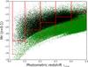Fig. 1 Rest-frame r-band absolute magnitude Mr vs. photometric redshift zphot for DR12 galaxies with r< 20.4 (black dots) and Stripe 82 galaxies with r< 22.4 (green dots), in areas with Herschel-SPIRE coverage. For clarity, only 20% of the DR12 sample and 10% of the Stripe 82 sample are plotted. The red boxes indicate the volume-limited subsamples in five redshift slices (solid: DR12; dashed: Stripe 82).

2.2. Herschel survey 250 μm maps

The H-ATLAS survey conducted observations at 100, 160, 250, 350, and 500 μm of the three equatorial fields also observed in the GAMA spectroscopic survey (Driver et al. 2011); these equatorial fields are G09, G12, and G15 centred at a right ascension of ~9, 12, and 15 h, respectively. For this study, we cut out a rectangle inside each of the GAMA fields with a total area of 95.6 deg². The version of the data used in this paper is the Phase 1 version 3 internal data release. The SPIRE maps, which have unit of Jy/beam, were made using the methods described by Valiante et al. (in prep.). Large-scale structures and artefacts are removed by running the NEBULISER routine developed by Irwin (2010). We estimated the local background by fitting a Gaussian to the peak of the histogram of pixel values in 30×30 pixel boxes and subtracted this background from the raw map.

As the deeper SDSS Coadd catalogue is located in Stripe 82, we also used maps from the two Herschel surveys in the Stripe 82 region, i.e. the Herschel Stripe 82 Survey (HerS; Viero et al. 2014) and the HerMES Large-Mode Survey (HeLMS; Oliver et al. 2012). The joint HeRS and HeLMS areal coverage between −10° and 37° (RA) covers the subset of Stripe 82 that has the lowest level of Galactic dust emission (or cirrus) foregrounds. For this study, we combined 39.1 deg² in HeRS and 47.6 deg² in HeLMS, which are covered by the SDSS Coadd data. The SPIRE data, obtained from the Herschel Science Archive, were reduced using the standard ESA software and the custom-made software package, SMAP (Levenson et al. 2010; Viero et al. 2014). Maps were made using an updated version of SMAP/SHIM, which is an iterative map-maker designed to optimally separate large-scale noise from signal. Viero et al. (2013) provide greater detail on these maps.

3. Method

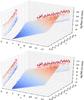Fig. 2 Top: estimated mean L250 as a function of the intrinsic population mean (μ) and standard deviation (σ) of log L250. For each set of (μ, σ), we generate ~2000 random numbers representing the 250 μm luminosities drawn from the log-normal distribution specified by (μ, σ). The estimates of the mean 250 μm luminosity are derived from these specific realisations of log-normal distributions. Bottom: the estimated standard deviation of L250 as a function of μ and σ.

Stacking was used for determining the mean properties of sources detected at another wavelength that are individually too dim to be detected at the working wavelength. For a given galaxy sample, we can stack¹ the 250 μm images centred at the positions of the galaxies weighted by luminosity distance squared (${\mathit{D}}_{\mathit{L}}^{\mathrm{2}}$) and k correction to derive the mean rest-frame 250 μm luminosity. To apply the k correction at rest-frame 250 μm, we used $\mathit{K}\mathrm{\left(}\mathit{z}\mathrm{\right)}\mathrm{=}{\left(\frac{{\mathit{\nu }}_{\mathrm{o}}}{{\mathit{\nu }}_{\mathrm{e}}}\right)}^{\mathrm{3}\mathrm{+}\mathit{\beta }}\frac{{\mathrm{e}}^{\mathit{h}{\mathit{\nu }}_{\mathrm{e}}\mathit{/}\mathit{k}{\mathit{T}}_{\mathrm{dust}}}\mathrm{-}\mathrm{1}}{{\mathrm{e}}^{\mathit{h}{\mathit{\nu }}_{\mathrm{o}}\mathit{/}\mathit{k}{\mathit{T}}_{\mathrm{dust}}}\mathrm{-}\mathrm{1}}\mathit{,}$(1)where ν_o is the observed frequency and ν_e = (1 + z)ν_o is the emitted frequency in the rest frame. We assumed a mean dust temperature of T_dust = 18.5 K and emissivity index β = 2, following Bourne et al. (2012).

In this paper, we extend the traditional stacking method to reconstruct the LF. The key assumption is that the rest-frame 250 μm luminosities L₂₅₀ of galaxies in a narrow bin of z and M_r follow a log-normal distribution, i.e. the logarithm of the luminosities, log L₂₅₀, follow a normal distribution with mean μ and standard deviation σ. In contrast, we used to m denote the mean of L₂₅₀ and s to denote the standard deviation of L₂₅₀. The two sets of parameters can be related to each other as, $\mathit{\mu }\mathrm{=}\ln \mathrm{(}\mathit{m}\mathit{/}\sqrt{\mathrm{1}\mathrm{+}{\mathit{s}}^{\mathrm{2}}\mathit{/}{\mathit{m}}^{\mathrm{2}}}\mathrm{)}\mathit{,\sigma }\mathrm{=}\sqrt{\ln \mathrm{(}\mathrm{1}\mathrm{+}{\mathit{s}}^{\mathrm{2}}\mathit{/}{\mathit{m}}^{\mathrm{2}}\mathrm{)}}\mathit{.}$(2)With stacking, we can estimate the mean of L₂₅₀ () and the standard deviation of L₂₅₀ (). We use m and s to denote the intrinsic population mean and standard deviation parameters, and and to denote estimates² of the intrinsic parameters.

To recover the LF in a given redshift bin, we need to infer μ and σ as a function of M_r, using combinations of and . In Fig. 2, we plot the estimated mean and standard deviation of L₂₅₀, i.e. and as a function of the intrinsic population mean and standard deviation of log L₂₅₀, i.e. μ and σ. To make this plot, we generated ~2000 random numbers (representing the 250 μm luminosities) drawn from a log-normal distribution for each set of (μ, σ) values. The estimates and were derived from these specific samples (i.e. realisations) of log-normal distributions. The estimates and become noisy when σ is large (even in the absence of noise), even though m and s can be related to μ and σ analytically (Eq. (2)). This is because and are sensitive to the large values in the tail of the distribution. To take the effect of realistic noise into account, we injected synthetic galaxies with log-normally distributed L₂₅₀ (drawn from distributions of known μ and σ) at random locations in the map. We can then measure the mean and standard deviation of L₂₅₀ from the stacks of synthetic galaxies in the presence of realistic noise and compare with the estimated mean and standard deviation of L₂₅₀ from the stacks of real galaxies. We summarise the main steps of recovering the 250 μm LF using our modified stacking method in Appendix A.

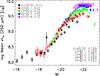Fig. 3 Mean rest-frame 250 μm luminosity L250 vs. Mr for the DR12 (solid squares) and Stripe 82 galaxies (open stars) in five redshift bins. Error bars correspond to the error on the mean.

4. Results

Figure 3 shows the mean rest-frame 250 μm luminosity L₂₅₀ as a function of M_r for the DR 12 and Stripe 82 galaxies. There is good agreement in the overlapping M_r range; this agreement is generally below 0.1 dex difference. At the faint end, galaxies exhibit a steep correlation between L₂₅₀ and M_r without significant evolution with redshift. At the bright end, the mean L₂₅₀ as a function of M_r begins to flatten with significant redshift evolution. As optically red galaxies dominate at the bright end, the redshift evolution can be explained by the evolution in the red galaxy population, which was first observed in Bourne et al. (2012). In the two highest redshift bins, z4 and z5, the depth of DR 12 means that we are only able to probe the bright galaxies with a flattened relation between the mean L₂₅₀ and M_r. As explained in Appendix A, our method only works if there is a roughly monotonic relation between the mean L₂₅₀ and M_r. Therefore, we do not use DR 12 at z> 0.3. Figure 4 shows our reconstructed rest-frame 250 μm LF, using DR 12 in the GAMA fields and the deeper Coadd data in Stripe 82. The luminosity limit reached by our method corresponds to the mean L₂₅₀ of the galaxies in the faintest M_r bin in each redshift slice. Good agreement can be found between our results and previous determinations in the overlapping luminosity range. The dashed line in each panel is a modified Schechter function (Saunders et al. 1990) fit to our results (in the GAMA fields and Stripe 82) and measurements from Marchetti et al. (2015), $\mathit{\phi }\mathrm{\left(}\mathit{L}\mathrm{\right)}\mathrm{=}\frac{\mathrm{d}\mathit{n}}{\mathrm{d}\mathit{L}}\mathrm{=}{\mathit{\phi }}^{\mathrm{\ast }}{\left(\frac{\mathit{L}}{{\mathit{L}}^{\mathrm{\ast }}}\right)}^{\mathrm{1}\mathrm{-}\mathit{\alpha }}\exp \left[\mathrm{-}\frac{\mathrm{1}}{\mathrm{2}{\mathit{\sigma }}^{\mathrm{2}}}{\log }_{\mathrm{10}}^{\mathrm{2}}\left(\mathrm{1}\mathrm{+}\frac{\mathit{L}}{{\mathit{L}}^{\mathrm{\ast }}}\right)\right]\mathit{,}$(3)where φ^∗ is the characteristic density, L^∗ is the characteristic luminosity, α describes the faint-end slope, and σ controls the shape of the cut-off at the bright end. We assume σ and α do not change with redshift. Table 1 lists the best-fit and marginalised error for the parameters in the modified Schechter function. We find strong positive luminosity evolution ${\mathit{L}}_{\mathrm{250}}^{\mathrm{\ast }}\mathrm{\left(}\mathit{z}\mathrm{\right)}\mathrm{\propto }\mathrm{(}\mathrm{1}\mathrm{+}\mathit{z}{\mathrm{)}}^{\mathrm{4.89}\mathrm{\pm }\mathrm{1.07}}$ and moderate negative density evolution ${\mathrm{\Phi }}_{\mathrm{250}}^{\mathrm{\ast }}\mathrm{\left(}\mathit{z}\mathrm{\right)}\mathrm{\propto }\mathrm{(}\mathrm{1}\mathrm{+}\mathit{z}{\mathrm{)}}^{\mathrm{-}\mathrm{1.02}\mathrm{\pm }\mathrm{0.54}}$ over 0.02 <z< 0.5.

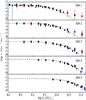Fig. 4 250 μm LF in five redshift bins. Our results are plotted as filled stars (black: Stripe 82; red: GAMA fields), which agree well with previous measurements (green circles: Dye et al. 2010; blue circles: Marchetti et al. 2015). The dashed line is the best fit to our measurements (GAMA fields and Stripe 82) and Marchetti et al. (2015).

5. Conclusion

We study the low-redshift, rest-frame 250 μm LF using stacking of deep optically selected galaxies from the SDSS survey on the Herschel-SPIRE maps of the GAMA fields and the Stripe 82 area. Our method not only recovers the mean 250 μm luminosities L₂₅₀ of galaxies that are too faint to be individually detected, but also their underlying distribution functions. We find very good agreement with previous measurements. More importantly, our stacking method probes the LF down to much fainter luminosities (~ 25 times fainter) than achieved by previous efforts. We find strong positive luminosity evolution ${\mathit{L}}_{\mathrm{250}}^{\mathrm{\ast }}\mathrm{\left(}\mathit{z}\mathrm{\right)}\mathrm{\propto }\mathrm{(}\mathrm{1}\mathrm{+}\mathit{z}{\mathrm{)}}^{\mathrm{4.89}\mathrm{\pm }\mathrm{1.07}}$ and moderate negative density evolution ${\mathrm{\Phi }}_{\mathrm{250}}^{\mathrm{\ast }}\mathrm{\left(}\mathit{z}\mathrm{\right)}\mathrm{\propto }\mathrm{(}\mathrm{1}\mathrm{+}\mathit{z}{\mathrm{)}}^{\mathrm{-}\mathrm{1.02}\mathrm{\pm }\mathrm{0.54}}$ at z< 0.5. Our method bypasses some major difficulties in previous studies, however, it critically relies on the input photometric redshift catalogue. Therefore, issues such as photometric redshift bias and accuracy would have an impact. Over the coming years, our stacking method of reconstructing the LF will deliver even more accurate results and also extend to even fainter luminosities and higher redshifts. This is because, although we are probably not going to have any FIR/sub-mm imaging facility that will surpass Herschel in terms of areal coverage, sensitivity, and resolution in the near future, our knowledge of the optical and near-IR Universe will increase dramatically with ongoing and planned surveys such as DES and LSST. In addition, large and deep spectroscopic surveys such as EUCLID and DESI will further improve the quality of photometric redshift.

Acknowledgments

P.N. acknowledges the support of the Royal Society through the award of a University Research Fellowship, the European Research Council, through receipt of a Starting Grant (DEGAS-259586) and the support of the Science and Technology Facilities Council (ST/L00075X/1). N.B. acknowledges funding from the European Union Seventh Framework Programme (FP7/2007-2013) under grant agreement No. 312725. L.D. and S.J.M. acknowledge support from the European Research Council Advanced Investigator grant, COSMICISM and Consolidator grant, cosmic dust. The H-ATLAS is a project with Herschel, which is an ESA space observatory with science instruments provided by European-led Principal Investigator consortia and with important participation from NASA. The H-ATLAS web site is http://www.h-atlas.org/. Funding for SDSS-III has been provided by the Alfred P. Sloan Foundation, the Participating Institutions, the National Science Foundation, and the US Department of Energy Office of Science. The SDSS-III web site is http://www.sdss3.org/. SDSS-III is managed by the Astrophysical Research Consortium for the Participating Institutions of the SDSS-III Collaboration including the University of Arizona, the Brazilian Participation Group, Brookhaven National Laboratory, Carnegie Mellon University, University of Florida, the French Participation Group, the German Participation Group, Harvard University, the Instituto de Astrofisica de Canarias, the Michigan State/Notre Dame/JINA Participation Group, Johns Hopkins University, Lawrence Berkeley National Laboratory, Max Planck Institute for Astrophysics, Max Planck Institute for Extraterrestrial Physics, New Mexico State University, New York University, Ohio State University, Pennsylvania State University, University of Portsmouth, Princeton University, the Spanish Participation Group, University of Tokyo, University of Utah, Vanderbilt University, University of Virginia, University of Washington, and Yale University.

References

Appendix A: The modified stacking method

Below we summarise the main steps of recovering the 250 μm LF in a given redshift bin using our modified stacking method:

• 1.

  Stack the 250 μm images centred on the galaxies in a given M_r bin, weighted by luminosity distance squared (${\mathit{D}}_{\mathit{L}}^{\mathrm{2}}$) and k-correction. Measure the mean and standard deviation of the rest-frame 250 μm luminosity L₂₅₀, i.e. and . Note that the estimates and are affected by instrument noise in the 250 μm images.

• 2.

  Generate n bootstrap realisations for each sample (i.e. the set of galaxies in a given M_r bin) and repeat Step 1 for all realisations. Form an estimate of the error on and , using the n bootstrap realisations.

• 3.

  Generate synthetic galaxies³ with random L₂₅₀ values drawn from log-normal distributions set by known μ and σ values and add them to random locations in the map. The σ values (i.e. the standard deviation of log L_IR) are chosen to sample linearly between 0.027 and 2.17 with a width of 0.027. The μ values (i.e. the mean of log L_IR) are sampled linearly between 6.478 and 12.088 with a width of 0.035. Measure the mean and standard deviation of L₂₅₀ of the synthetic galaxies, taking into account the effect of instrument noise in the 250 μm images.

• 4.

  By comparing the measured mean and standard deviation of L₂₅₀ of the real galaxies with the mean and standard deviation estimates of the synthetic galaxies (for all n repetitions), select all sets of μ and σ values that give reasonably close mean and standard deviation to the real values using χ² statistics.

• 5.

  For each set from the accepted μ and σ values, generate log-normally distributed L₂₅₀ and assign them randomly to galaxies in a given M_r bin. Calculate the resulting distribution function of L₂₅₀.

• 6.

  Repeat Step 6 for all accepted values of μ and σ, so we have multiple realisations of the distribution function of L₂₅₀ for galaxies in a single M_r bin.

• 7.

  Repeat Step 1 to 7 for all M_r bins. The 250 μm LF is derived by adding up contributions to a given L₂₅₀ bin from galaxies in all M_r bins. Using the multiple realisations, form a median estimate of the final 250 μm LF and its confidence range.

For this method to work properly, it is important that the mean r-band luminosity M_r and the mean 250 μm luminosity has a more or less monotonic relation. Otherwise, one could have situations where some sources in a given bin in L₂₅₀ have fainter M_r values than are included in the optical prior list. Our method is similar to the stacking approach in Béthermin et al. (2012) which was used to derive the SPIRE number counts. The main difference is that, in Béthermin et al. (2012), the aim was to recover the mean and standard deviation of the logarithm of the 250 μm flux rather than luminosity.

All Tables

All Figures

Fig. 1 Rest-frame r-band absolute magnitude Mr vs. photometric redshift zphot for DR12 galaxies with r< 20.4 (black dots) and Stripe 82 galaxies with r< 22.4 (green dots), in areas with Herschel-SPIRE coverage. For clarity, only 20% of the DR12 sample and 10% of the Stripe 82 sample are plotted. The red boxes indicate the volume-limited subsamples in five redshift slices (solid: DR12; dashed: Stripe 82).

In the text

Fig. 2 Top: estimated mean L250 as a function of the intrinsic population mean (μ) and standard deviation (σ) of log L250. For each set of (μ, σ), we generate ~2000 random numbers representing the 250 μm luminosities drawn from the log-normal distribution specified by (μ, σ). The estimates of the mean 250 μm luminosity are derived from these specific realisations of log-normal distributions. Bottom: the estimated standard deviation of L250 as a function of μ and σ.

In the text

	Fig. 3 Mean rest-frame 250 μm luminosity L250 vs. Mr for the DR12 (solid squares) and Stripe 82 galaxies (open stars) in five redshift bins. Error bars correspond to the error on the mean.
In the text

	Fig. 4 250 μm LF in five redshift bins. Our results are plotted as filled stars (black: Stripe 82; red: GAMA fields), which agree well with previous measurements (green circles: Dye et al. 2010; blue circles: Marchetti et al. 2015). The dashed line is the best fit to our measurements (GAMA fields and Stripe 82) and Marchetti et al. (2015).
In the text

References

- Alam, S., Albareti, F. D., Allen de Prieto, C., et al. 2015, ApJS, 219, 12 [NASA ADS] [CrossRef] [Google Scholar]
- Annis, J., Soares-Santos, M., Strauss, M. A., et al. 2014, ApJ, 794, 120 [NASA ADS] [CrossRef] [Google Scholar]
- Bavouzet, N., Dole, H., Le Floc’h, E., et al. 2008, A&A, 479, 83 [NASA ADS] [CrossRef] [EDP Sciences] [Google Scholar]
- Beck, R., Dobos, L., Budavári, T., Szalay, A. S., & Csabai, I. 2016, MNRAS, 460, 1371 [NASA ADS] [CrossRef] [Google Scholar]
- Béthermin, M., Dole, H., Beelen, A., & Aussel, H. 2010, A&A, 512, A78 [NASA ADS] [CrossRef] [EDP Sciences] [Google Scholar]
- Béthermin, M., Le Floc’h, E.,Ilbert, O., et al. 2012, A&A, 542, A58 [NASA ADS] [CrossRef] [EDP Sciences] [Google Scholar]
- Blanton, M. R., & Roweis, S. 2007, AJ, 133, 734 [NASA ADS] [CrossRef] [Google Scholar]
- Bourne, N., Maddox, S. J., Dunne, L., et al. 2012, MNRAS, 421, 3027 [NASA ADS] [CrossRef] [Google Scholar]
- Casey, C. M., Berta, S., Béthermin, M., et al. 2012, ApJ, 761, 140 [NASA ADS] [CrossRef] [Google Scholar]
- Casey, C. M., Narayanan, D., & Cooray, A. 2014, Phys. Rep., 541, 45 [NASA ADS] [CrossRef] [Google Scholar]
- Csabai, I., Dobos, L., Trencséni, M., et al. 2007, Astron. Nachr., 328, 852 [NASA ADS] [CrossRef] [Google Scholar]
- Devlin, M. J., Ade, P. A. R., Aretxaga, I., et al. 2009, Nature, 458, 737 [NASA ADS] [CrossRef] [PubMed] [Google Scholar]
- Dobos, L., Csabai, I., Yip, C.-W., et al. 2012, MNRAS, 420, 1217 [NASA ADS] [CrossRef] [Google Scholar]
- Dole, H., Lagache, G., Puget, J.-L., et al. 2006, A&A, 451, 417 [NASA ADS] [CrossRef] [EDP Sciences] [MathSciNet] [Google Scholar]
- Driver, S. P., Hill, D. T., Kelvin, L. S., et al. 2011, MNRAS, 413, 971 [NASA ADS] [CrossRef] [Google Scholar]
- Dye, S., Dunne, L., Eales, S., et al. 2010, A&A, 518, L10 [NASA ADS] [CrossRef] [EDP Sciences] [Google Scholar]
- Eales, S., Chapin, E. L., Devlin, M. J., et al. 2009, ApJ, 707, 1779 [NASA ADS] [CrossRef] [Google Scholar]
- Eales, S., Dunne, L., Clements, D., et al. 2010a, PASP, 122, 499 [NASA ADS] [CrossRef] [Google Scholar]
- Eales, S. A., Raymond, G., Roseboom, I. G., et al. 2010b, A&A, 518, L23 [NASA ADS] [CrossRef] [EDP Sciences] [Google Scholar]
- Griffin, M. J., Abergel, A., Abreu, A., et al. 2010, A&A, 518, L3 [Google Scholar]
- Hauser, M. G., & Dwek, E. 2001, ARA&A, 39, 249 [NASA ADS] [CrossRef] [Google Scholar]
- Lacey, C. G., Baugh, C. M., Frenk, C. S., et al. 2015, MNRAS, submitted [arXiv:1509.08473] [Google Scholar]
- Marchetti, L., Vaccari, M., Franceschini, A., et al. 2016, MNRAS, 456, 1999 [NASA ADS] [CrossRef] [Google Scholar]
- Oliver, S. J., Bock, J., Altieri, B., et al. 2012, MNRAS, 424, 1614 [NASA ADS] [CrossRef] [EDP Sciences] [Google Scholar]
- Pilbratt, G. L., Riedinger, J. R., Passvogel, T., et al. 2010, A&A, 518, L1 [CrossRef] [EDP Sciences] [Google Scholar]
- Reis, R. R. R., Soares-Santos, M., Annis, J., et al. 2012, ApJ, 747, 59 [NASA ADS] [CrossRef] [Google Scholar]
- Schaye, J., Crain, R. A., Bower, R. G., et al. 2015, MNRAS, 446, 521 [Google Scholar]
- Schlegel, D. J., Finkbeiner, D. P., & Davis, M. 1998, ApJ, 500, 525 [NASA ADS] [CrossRef] [Google Scholar]
- Symeonidis, M., Vaccari, M., Berta, S., et al. 2013, MNRAS, 431, 2317 [NASA ADS] [CrossRef] [Google Scholar]
- Vaccari, M., Marchetti, L., Franceschini, A., et al. 2010, A&A, 518, L20 [NASA ADS] [CrossRef] [EDP Sciences] [Google Scholar]
- Viero, M. P., Asboth, V., Roseboom, I. G., et al. 2014, ApJS, 210, 22 [NASA ADS] [CrossRef] [Google Scholar]