| Issue |
A&A
Volume 592, August 2016
|
|
|---|---|---|
| Article Number | A38 | |
| Number of page(s) | 7 | |
| Section | Cosmology (including clusters of galaxies) | |
| DOI | https://doi.org/10.1051/0004-6361/201527776 | |
| Published online | 18 July 2016 | |
Probing scalar tensor theories for gravity in redshift space
1 Korea Astronomy and Space Science Institute, Yuseong-gu, 305-348 Daejeon, Korea
e-mail: csabiu@kasi.re.kr
2 School of Physics, Korea Institute for Advanced Study, Dongdaemun-gu, 130-722 Seoul, Korea
3 Institute of theoretical astrophysics, University of Oslo, 0315 Oslo, Norway
4 Institute for Computational Cosmology, Department of Physics, Durham University, Durham DH1 3LE, UK
Received: 18 November 2015
Accepted: 20 May 2016
We present measurements of the spatial clustering statistics in redshift space of various scalar field modified gravity simulations. We utilise the two-point and three-point correlation functions to quantify the spatial distribution of dark matter halos within these simulations and thus discriminate between the models. We compare Λ cold dark matter (ΛCDM) simulations to various modified gravity scenarios and find consistency with previous work in terms of two-point statistics in real and redshift space. However, using higher-order statistics such as the three-point correlation function in redshift space we find significant deviations from ΛCDM hinting that higher-order statistics may prove to be a useful tool in the hunt for deviations from General Relativity.
Key words: cosmology: theory / gravitation / large-scale structure of Universe
© ESO, 2016
1. Introduction
The Λ cold dark matter (ΛCDM) cosmological model has been shown to reproduce many observational measurements, from the CMB at very early times to the late time clustering of galaxies. Despite the successes of the model, certain issues remain to be fully explained. These are either conceptual or arise from conflict with observational constraints. One of the main problems is that the nature of the two main ingredients of the model (dark matter and dark energy) remains unknown. Among the different solutions to the philosophical and quantitative inconsistencies associated with these components is the idea of modifying the gravitational theory. Several alternative theories exist (Clifton et al. 2012; Amendola et al. 2013), all of which include extra degrees of freedom in the form of scalar, vector, or even tensor fields. As General Relativity (GR) is proven to be valid to high accuracy on solar system scales (Will 2014), any modification introduced must reduce to GR in these scales, which is done through screening mechanisms. Within the context of scalar-tensor theories, there are three such mechanisms based on conformal couplings, namely Vainshtein (Vainshtein 1972), Symmetron (Hinterbichler & Khoury 2010), and Chameleon (Khoury & Weltman 2004). In addition, Koivisto et al. (2012) has recently proposed a mechanism based on a disformal coupling.
Since all the above modified gravity models with screening mechanisms seem to be viable, the question arises of how to distinguish between the different models using cosmological observations. Since the effects of the forces associated with the extra degree of freedom emerge during the onset of non-linear structure formation, it is a promising tool that can be used to rule out some of the above models. The non-linear effects arising from these screening mechanisms have been studied using cosmological N-body simulations (Oyaizu 2008; Schmidt 2009; Li et al. 2011; Lombriser et al. 2013; Boehmer & Mota 2008; Zhao et al. 2011a,b; Barreira et al. 2013).
Second-order clustering statistics have been used to investigate differences between ΛCDM and modified gravity models, particularly those of Hinterbichler et al. (2011), Brax et al. (2011), Jennings et al. (2012) and Brax et al. (2012). Recently Song et al. (2015) have put observational bounds on fR0 using SDSS data. Another novel technique for probing modified gravity involving second-order statistics was investigated by Lombriser et al. (2015) using the density-field clipping method (Simpson et al. 2011, 2013). They found that constraints on f(R) gravity can be tightened when clipping the density field with a high threshold since contributions of screened high-density regions to the matter power spectrum will be reduced and will boost the modified gravity effects.
In this paper we focus on higher-order clustering statistics in redshift space as a tool for differentiating modified gravity models (as alternatives to dark energy) from a fiducial GR model. Three-point functions were studied in the linear regime for general scalar tensor theories ranging from galileons to the most general Horndeski model (Bartolo et al. 2013; Takushima et al. 2014; Bellini et al. 2015). The non-linear regime was studied by Gil-Marín et al. (2011) in the f(R) case. Here we repeat the calculations for the same f(R) model, but extend this previous study in two ways. Firstly, we run simulations with a code that includes an adaptive mesh refinement structure (AMR) giving a much more accurate description of the clustering, especially on small scales. Secondly, we focus our study not only on the real space correlation functions, but also on the redshift space functions, which are ultimately the ones that can be observed. Furthermore, we also present predictions for the symmetron model in addition to f(R).
The paper is structured as follows. In Sect. 2 we discuss the scalar field models investigated and briefly describe the numerical simulations used. In Sect. 3 we lay out our framework for analysing the numerical simulations and discuss our specific implementation of the two- and three-point clustering statistics that we use. We present our clustering results for the various models in Sect. 4, and conclude in Sect. 5.
2. Models and simulations
2.1. Gravitational models
We focus our analysis on two specific scalar tensor models: the symmetron model and a particular case of f(R) theories. Both models include screening mechanisms, which reduce them to GR in high-density regions and thus make them able to pass solar system tests. Below we summarise the characteristics of the models. In both cases, we work in the Einstein frame and so Einstein’s equation will be unchanged. The dominant dynamical effects will appear as a modification of the geodesics equation that is used to track the motion of the particles, which now will include a fifth force term.
2.1.1. The symmetron model
The symmetron model was originally discussed in Pietroni (2005), Olive & Pospelov (2008) and Hinterbichler & Khoury (2010) as a standard scalar tensor model which has a particular coupling to matter. The model includes a screening mechanism based on the restoration of a particular symmetry. The cosmology of this model at the background and linear perturbation level has been studied in Hinterbichler et al. (2011) and Brax et al. (2011). In the non-linear case, there are several results coming from quasi-static non-linear N-body cosmological simulations (Davis et al. 2012; Brax et al. 2012; Llinares et al. 2014). The effect of non-static terms in these simulations was presented in Llinares & Mota (2013, 2014).
The action of the symmetron model is given by ![\begin{eqnarray} S = \int \sqrt{-g} \left[ {\frac{M_{\rm Pl}^2}{2}} R - \frac{1}{2}\nabla^a\phi \nabla_a \phi - V(\phi)\right] {\rm d}^4x + S_{M}(\tilde{g}_{ab}, \psi) , \label{symm-action} \end{eqnarray}](/articles/aa/full_html/2016/08/aa27776-15/aa27776-15-eq6.png) (1)where R is the Ricci scalar, the Einstein and Jordan frame metrics (gab and
(1)where R is the Ricci scalar, the Einstein and Jordan frame metrics (gab and  ) are conformally related
  (2)and SM is the matter action which describes the evolution of the matter fields ψ. The potential and conformal factor that define the model are
 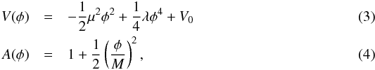 where μ and M are mass scales, λ is a dimensionless constant, and V0 is tuned to match the observed cosmological constant. The equation of motion for the scalar field that comes out from the action is then
 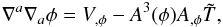 (5)where
 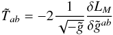 (6)is the Jordan frame energy momentum tensor (here, LM is the Lagrangian matter). By fixing the metric to be a perturbed Friedmann-Robertson-Walker metric
  (7)where Φ is a scalar perturbation (i.e. the gravitational potential in a classical context), we can write the equation of motion of the scalar field in the form
 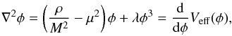 (8)where ρ is the Jordan frame matter density and the effective potential is given by
 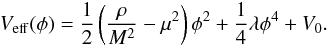 (9)From this equation, it is possible to see that the expectation value of the scalar field vanishes at high matter densities. This sets the conformal factor A to unity and thus decouples the scalar from the matter, producing the screening of the fifth force.
For numerical convenience, we work with a dimensionless scalar field χ ≡ φ/φ0, where φ0 is the expectation value for ρ = 0:  (10)We also substitute the three free parameters (M,μ,λ) and use instead the range of the field that corresponds to ρ = 0,
  (11)a dimensionless coupling constant,
  (12)and the scale factor at the time of symmetry breaking,
  (13)where ρ0 is the background density at z = 0. Throughout the paper we use either aSSB or its associated redshift zSSB. The equation for the dimensionless scalar field χ is then
 ![\begin{eqnarray} \nabla^2\chi = \frac{a^2}{2\lambda_0^2}\left[\left(\frac{\rho}{\rho_{\rm SSB}} - 1\right)\chi + \chi^3 \right]. \label{eq_motion_chi} \end{eqnarray}](/articles/aa/full_html/2016/08/aa27776-15/aa27776-15-eq40.png) (14)In the Einstein frame, the effects of the scalar field on the matter distribution will be given by a modification of the geodesics equation, which takes the following form:
(14)In the Einstein frame, the effects of the scalar field on the matter distribution will be given by a modification of the geodesics equation, which takes the following form:  (15)Here H0 is the Hubble parameter at redshift z = 0, Ωm is the mean matter density at redshift z = 0 normalised to the critical density, and the dots represent derivatives with respect to Newtonian time defined by Eq. (7).
2.1.2. The f(R) model
Among the large number of f(R) models that exist in the literature we choose the model presented in Hu & Sawicki (2007), which has attracted great interest in the context of dark energy models (see Lombriser 2014 for a review on observational constraints on the model). In the context of non-linear structure formation that we study here, there are several N-body codes capable of simulating this model (Oyaizu 2008; Li et al. 2012; Puchwein et al. 2013; Llinares et al. 2014). The validity of the quasi-static approximation assumed in these codes was studied in detail in the linear and non-linear regime in Noller et al. (2014) and Bose et al. (2015).
The action that defines the model is ![\begin{eqnarray} S = \int \sqrt{-g} \left[ \frac{R+f(R)}{16\pi G} + L_{M} \right] {\rm d}^4 x, \end{eqnarray}](/articles/aa/full_html/2016/08/aa27776-15/aa27776-15-eq44.png) (16)where the free function f is chosen as
(16)where the free function f is chosen as  (17)where
  and c1, c2, and n are dimensionless model parameters. By requiring the model to give dark energy, it is possible to reduce the number of free parameters from three to two (n and fR0). This requirement translates into
  (18)where ΩΛ is the density parameter associated with the cosmological constant. Instead of using c1 (or c2) as the second free parameter, it is convenient to use
  (19)which relates to the range of fifth force in the cosmological background at redshift z = 0 as
  (20)where
  is the range of the field, which is typically given in Mpc/h. It has been shown that the model can be translated into a scalar tensor model (Brax et al. 2008). This can be done by applying a conformal transformation
  (21)where
  (22)with
  . We also define
  (23)This equation defines R(φ), which can be used to get the potential V(φ) in which the scalar field oscillates and that is given by
  (24)In the static limit, the scalar field fR fulfils the following equation of motion,
 ![\begin{eqnarray} \nabla^2f_R &= &-\frac{1}{a}\Omega_{\rm m} H_0^2\left(\eta - 1\right) + a^2\Omega_{\rm m} H_0^2 \nonumber\\ &&\times \left[\left(1+4\frac{\Omega_\Lambda}{\Omega_{\rm m}}\right)\left(\frac{f_{R0}}{f_R}\right)^{\frac{1}{n+1}} - \left(a^{-3} + 4\frac{\Omega_\Lambda}{\Omega_{\rm m}}\right)\right], \end{eqnarray}](/articles/aa/full_html/2016/08/aa27776-15/aa27776-15-eq65.png) (25)where fR0 is the value that corresponds to the minimum for the background density today and η is the local matter density in units of the mean density of the Universe.
(25)where fR0 is the value that corresponds to the minimum for the background density today and η is the local matter density in units of the mean density of the Universe.
The geodesic equation takes the form (26)where we obtain an extra term with respect to standard gravity which corresponds to the fifth force.
2.2. The N-body code
The simulations were run with the code Isis (Llinares et al. 2014), which is a modified gravity version of the code Ramses (Teyssier 2002). The code is a particle mesh code which includes adaptive mesh refinements and can thus increase the resolution of the solutions when needed (i.e. in the centre of the dark matter halos). In order to solve the equations for the scalar field, the code uses a non-linear version of the linear multigrid solver with which Ramses solves the Poisson equation. The solver works by doing Gauss-Seidel iterations on the discretised version of the equations to find improved solutions based on an initial guess. Given the multiscale properties of the problem, the solver also makes iterations on coarse grids, which can increase the speed of convergence by several orders of magnitude. The code is the only one present in the literature that can solve in an explicit way the scalar field equations out of the static limit. This non-static solver was already applied to symmetron and disformal gravity models (Llinares & Mota 2014; Hagala et al. 2016). A comparison between the accuracy of this code and other codes that solve the same set of equations can be found in Winther et al. (2015).
2.3. Simulations
The data to be used for the analysis was obtained from a set of simulations that were run with both standard gravity and the two modified gravity models. Table 1 summarises the model parameters. The initial conditions were generated assuming that the scalar field is fully screened at high redshift and thus, the Zel’dovich approximation is valid for all the models. To generate the only set of initial conditions we used the package Cosmics (Bertschinger 1995). The box size and number of particles employed are 256 Mpc/h and 5123. The background cosmology is also the same for all the simulations and is defined as a flat ΛCDM model given by (Ωm,ΩΛ,H0) = (0.267,0.733,71.9 km s-1 Mpc-1). The simulations are normalised using the linearly extrapolated value of σ8 at redshift zero. All the simulations have the same normalisation, which is necessary if we want all the simulations to be consistent with the CMB. The simulations were run up to redshift zero, which is the moment at which we make our analysis. Furthermore, all the simulations use the same background cosmology with exactly the same initial conditions (i.e. with the same initial seed for the random numbers generator). Thus we assume the effects of the scalar field appear only because of the existence of a fifth force in the perturbation level.
The power spectrum of the initial conditions are not normalised to CMB measurements, but rather are normalised using a redshift zero σ8, which is evolved back in time with linear Newtonian theory. This is a standard approach within the community; however, this method has the drawback that the final normalisation of the simulation cannot be completely controlled owing to the presence of the fifth force in the modified gravity models. In all cases, even changes in clustering amplitudes should be investigated within the domain of modified gravity theories.
In order to investigate the clustering of dark matter halos, we make use of halo catalogues that were obtained with the phase-space, friends-of-friends (FOF) code Rockstar (Behroozi et al. 2013). The samples used for the analysis include all the halos reported by the halo finder with no discrimination between virialized and non-virialized objects. The halo catalogue has a cut-off for low-mass halos at 20 particles per halo, which corresponds to a minimum halo mass of 1.85 × 10¹¹M⊙/h. The same cut-off was used for all the simulations. We have compared the halo mass function from these simulations with higher resolution simulations and with theoretical models and find no bias in using 20 particles to define the halos.
For details on the implementation of the modified equations on the code Isis and on the simulations we refer the reader to Llinares et al. (2014).
Model parameter values.
3. Correlation statistics
We want to quantify the spatial clustering of the simulated halos so that comparisons between models are easier to perform. To achieve this we calculate the two- and three-point correlation functions using well-known estimators, which are described below.
3.1. Two-point correlation function
We estimate the full two-point correlation function (2PCF) of the DM halo distribution in each of the simulations listed in Table 1. The 2PCF is estimated in real and redshift space and in both isotropic and anisotropic σ,π-decompositions. The correlation functions are calculated using the “Landy-Szalay” estimator (Landy & Szalay 1993), (27)where DD(r) is the number of data-data pairs, DR the number of data-random pairs, and RR is the number of random-random pairs, all separated by a displacement vector r and properly normalised. In the isotropic case we measure ξ(r) with no angular dependence and we choose the binning r = 0 → 60 Mpc/h in 20 linearly spaced bins. The number of random particles used to define the unclustered reference sample is ≈20 times the number of halo particles. This is done to reduce statistical fluctuation due to Poisson noise in the random pair counting.
In the anisotropic analysis we decompose the vector r into a line-of-sight distance component σ and a perpendicular component π. Then we proceed to measure ξ(σ,π) from σ and π = 0 → 60 Mpc in 15 linearly spaced bins, resulting in 225 bins in the σ−π space.
3.2. Three-point correlation function
Higher-order correlations are usually denoted ξn(r1,...,rn), where n is the order of the correlation function. As an example, the 3PCF is defined as the joint probability of there being a galaxy in each of the volume elements dV1, dV2, and dV3 given that these elements are arranged in a configuration defined by the sides of the triangle, r1, r2, and r3. The joint probability can be written as![\begin{equation} {\rm d}P_{1,2,3}=\bar{n}^{3}[1+\xi({\vec r}_{1})+\xi({\vec r}_{2})+\xi({\vec r}_{3})+\zeta({\vec r}_{1},{\vec r}_{2},{\vec r}_{3})]{\rm d}V_{1}{\rm d}V_{2}{\rm d}V_{3}. \label{eq:3PCF} \end{equation}](/articles/aa/full_html/2016/08/aa27776-15/aa27776-15-eq101.png) (28)The expression above consists of several parts: the sum of correlations for each side of the triangle and ζ, the full three-point correlation function, and
(28)The expression above consists of several parts: the sum of correlations for each side of the triangle and ζ, the full three-point correlation function, and  the mean density of data points. We utilise the 3PCF estimator of Szapudi & Szalay (1998),
  (29)where each term represents the normalised triplet counts in the data (D) and random (R) fields that satisfy a particular triangular configuration.
The 3PCF is computed in an isotropic (angle-averaged) way and is a function of three variables that uniquely define a triangular configuration. The shape parameters can either be the three sides of the triangle, (r1,r2,r3), or more commonly (s,q,θ), where  In Eq. (32),
  is the unit vector of side i of the triangle. The 3PCF is usually calculated in various configurations where s and q are fixed, while θ is varied from 0° to 180°.
In our analysis we focus on two triangular configurations, s,q = 2 Mpc /h, 1 and s,q = 3 Mpc /h, 2 with each probing eight equally spaced bins in cosθ. Our choice of scales was determined by practical and statistical issues. On small scales, baryonic physics can be significant; however, our simulations do not include these effects, so comparison to observation on scales less than 1 Mpc would be problematic. On larger scales the 3PCF amplitude drops off drastically and owing to the small box size of our simulation, the statistical noise becomes significant. We find through testing that s = 2, 3 Mpc and q = 1, 2 give stable results.
4. Results
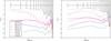 |
Fig. 1 left: fractional difference between the 2PCF measurements of dark matter halos within modified gravity and ΛCDM simulations in real comoving space. right: same as left plot, now in redshift space. |
In this section we will present the results of our clustering statistics for the various models, in real and redshift spaces.
4.1. Two-point function results
In Fig. 1 we show the relative difference Δξ = (ξmod−ξΛCDM) /ξΛCDM between the 2PCF (calculated from Eq. (27)) of the modified gravity simulations (see Sect. 2) and the ΛCDM case. The left-hand plot shows the relative difference between the 2PCF of the dark matter halos in real comoving space, while the right-hand plot shows the 2PCF in redshift space.
The errors on ξ(r) were derived using the jackknife method Scranton et al. (2002), which involves dividing the simulation box into N subsections with equal volume and then computing the mean and variance of ξ(r) from these N measurements of the correlation function with the ith region removed each time (where i = 1...N). In our analysis, we choose N = 27 and determine the variance from Lupton (1993),![\begin{equation} \sigma^2_\xi(r_i)=\frac{N_{jk}-1}{N_{jk}}\sum^{N_{jk}}_{k=1}[\xi_k(r_i)-\overline{\xi}(r_i)]^2, \end{equation}](/articles/aa/full_html/2016/08/aa27776-15/aa27776-15-eq124.png) (33)where Njk is the number of jackknife samples used and ri represents a single bin in the ξ(r) configuration space and
(33)where Njk is the number of jackknife samples used and ri represents a single bin in the ξ(r) configuration space and  is the mean of the jackknifed samples. Although not exact, the jackknife variance estimate will inform us if any deviations in the statistics between the ΛCDM model and modified gravity are significant and above the sampling noise. Of course, this variance will not inform us of the detectability of any deviation in a particular current or future observational dataset.
Considering first the real-space 2PCF in the left plot of Fig. 1 all the models, except for the weakest f(R) model FOFR6, show significant deviation from the ΛCDM case on scales <30 Mpc/h. In redshift space, we observe a similar amount of deviation from the ΛCDM case, with slightly more suppression on small scales.
The shapes of these curves suggest two things: the small-scale clustering amplitude of the modified gravity simulations may be slightly lower than that of ΛCDM, and the non-linear small-scale velocities may be higher in the modified gravity simulations, which would suppress clustering on small scales. Our results in Fig. 1 for the FOFR4 model appear consistent with the level of decrement observed in Taruya et al. (2014) where they find Δξ ≈ 13% on scales ~50 Mpc/h. The lower amplitude in both the real and redshift-space 2PCF is mainly due to the bias in the modified gravity simulation being lower than ΛCDM. This behaviour of the bias in modified gravity has already been suggested in the literature, where a decrease relative to ΛCDM in the dark matter halo bias in f(R) gravity was pointed out by Schmidt et al. (2009) and likewise for the galaxy bias by Fontanot et al. (2013). However, to fully understand this issue is beyond the scope of this paper; we thus focus our attention mainly on the differences between real and redshift-space quantities
So far we have looked at the isotropic 2PCF, however, this is not the most sensitive statistic to the redshift-space distortion effects. In Fig. 2 we show the anisotropic 2PCF in redshift space, decomposed into distances (σ,π), which correspond to directions across and along the line of sight.
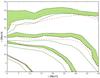 |
Fig. 2 Anisotropic, redshift-space, 2PCF measurements for three modified gravity simulations, using the dark matter halos in redshift space. For clarity we show only two extreme cases, FOFR4 (red dashed line) and SymmC (green solid line), and a mildly deviating model FOFR6 (light green dashed line). The four contour groups correspond to 2PCF values of [0.4, 0.1, 0.05, 0.01]. The green shaded region denotes the 1σ error bound around the ΛCDM value. |
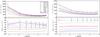 |
Fig. 3 left: Halo 3PCF for the eight simulations using the triangular configuration of s = 2 Mpc /h, q = 1, in real space. The full 3PCF is shown in the top panel, while the relative difference compared to ΛCDM is in the lower panel. right: same as right-hand panel, but in redshift space. |
The four contours correspond to the values [0.4, 0.1, 0.05, 0.01]. The green shaded region denotes the 1σ error bound around the ΛCDM value. For clarity we only show the clustering contours for three modified gravity models, two that exhibit the most deviation from ΛCDM (FOFR4 and SYMMC) and one that shows very similar clustering signal to ΛCDM (FOFR6). The various modified gravity simulations show very similar contours in this projection, although contours lying close to the line of sight exhibit some dispersion, i.e. a stronger fingers-of-god (FoG) effect compared to ΛCDM. Once again the FOFR4 model shows significant deviation from ΛCDM, especially on scales below 30 Mpc/h. However, it is the SYMMC model that shows the most dramatic deviation between the models investigated and ΛCDM. This effect means that owing to the presence of a fifth force, velocities are in general lager in modified gravity theories (Gronke et al. 2015; Hellwing et al. 2014). We note that redshift space distortions were already studied in f(R) gravity by Jennings et al. (2012); however, that work focuses its attention on the power spectrum of dark matter density perturbations.
4.2. Three-point function results
In the upper panels of Fig. 3 we show the 3PCF for all the simulations in the triangular configuration with s = 2 Mpc/h and q = 1, in real space (left panel) and redshift space (right panel). The length of the sides for this configuration are in the ranges 1.5 <r1< 2.5,1.5 <r2< 2.5,0 <r3< 5.
The lower panels of Fig. 3 show the relative difference, Δζ, between the 3PCF of ΛCDM and modified gravity, where Δζ = (ζmod−ζΛCDM) /ζΛCDM. The errorbars are once again estimated via 27 jackknife samples, and are basically determined by the comic variance of the structures within our 256 Mpc/h size simulation box. Nevertheless, smaller deviations between models can be significant in a comparison between simulations since all runs use the same phases and amplitudes in the initial conditions.
We can compare these results to Fig. 9 of Fosalba et al. (2005) who look at the same triangular configuration. Our results differ by a factor of ~4–8 because we consider the halo correlations, while in Fosalba et al. (2005) they consider the dark matter clustering, and also because the precise triangular binning scheme may differ between these two analyses.
We observe a dispersion between models which suggests that the 3PCF alone is at least as powerful a probe of modified gravitational clustering as the 2PCF. However, considering that the 3PCF is sensitive to the bias in a different way than the 2PCF, there may also be the potential to break any degeneracy between bias and modified gravity by using a combination of the 2PCF and 3PCF.
In real space the 3PCF of this triangular configuration shows mild deviation from the ΛCDM model. However, in redshift space, the 3PCF of this configuration shows a larger variation between models and all the modified gravity models deviate from ΛCDM; this is particularly evident in the FOFR models and SYMMD.
In Fig. 4 we investigate the 3PCF with triangular configuration s = 3 Mpc/h and q = 2. In this case the side lengths correspond to 2.5 <r1< 3.5,5.5 <r2< 6.5, and 2 <r3< 10 and thus this configuration will preferentially select triplets that occupy three distinct halos. However, in redshift space the FoG effect can bring in a one-halo contribution for “closed” and “open” triangles (i.e. when r3 is 3 and 9 Mpc/h, respectively), although the latter may be on too large a scale to add any significant effect. The one-halo contribution, within the halo model framework (Cooray & Sheth 2002), is the clustering signal in the 2PCF (or 3PCF) of pairs (or triplets) of galaxies residing in the same DM halo. This is opposed to the other contributions from galaxies residing in separate halos. In redshift space the clusters of galaxies can be elongated along the line of sight, thus the one-halo term can be significant on slightly larger scales than it would be in real-space.
In the left-hand panels of Fig. 4 we see that in real space the symmetron models are already significantly deviated from ΛCDM, while the FOFR models all lie within 1σ of ΛCDM. In redshift space, shown in the right panel, the models show a similar behaviour; however, the FOFR models have now diverged from ΛCDM. Interestingly the symmetron models A, B, and C do not show much relative difference between real and redshift space in contrast to SYMMD which shows a significant shift.
Our real space clustering measurements support the conclusion of Gil-Marín et al. (2011), where they find a weak dependence of the real space reduced bispectrum on | fR0 |. However in Gil-Marín et al. (2011) they look at scales outside the cluster size, i.e. k ≈ 0.4. In our work looking at the real and redshift-space full 3PCF on small scales, we find significant departures from the LCDM clustering. We suspect that this is due to the altered velocity distribution in modified gravity which results in anisotropic redshift space distortions that can be detected with higher-order clustering statistics. However, this claim should be tested further in future work.
5. Conclusions
We present the first measurements of the higher-order clustering in redshift space of certain modified gravity models. Using the three-point correlation function we are able to probe deviations in the clustering signal between modified gravity models and ΛCDM.
Owing to the volume and number of numerical simulations that we used, we show only a qualitative study of the higher-order clustering in redshift space. We have shown that the small-scale clustering in redshift space is significantly altered in the modified gravity models we consider compared to ΛCDM. This is especially true for higher-order statistics, namely the 3PCF.
In this work we have assumed a single set of cosmological parameters while varying the gravitational force; however, the effect of the modified gravity on the two- and three-point clustering should be quantified precisely and checked for any degeneracy with the cosmological parameters. This will require many N-body simulations and was therefore beyond the scope of our study; however, we hope that this work will prompt further research in this direction.
Acknowledgments
Several of the authors thank Arman Shafieloo, Stephen Appleby, Dhiraj Hazra, and the Asia Pacific Center for Theoretical Physics for their hospitality during their 1st joint workshop on Dark Energy, where this project was realised. We thank Prof. Juhan Kim for advising us on the halo mass function in our N-body simulations. We also thank the anonymous referee for very helpful comments and suggestions. D.F.M. acknowledges support from the Research Council of Norway. C.L.L. acknowledges support from the Research Council of Norway through grant 216756 and from STFC consolidated grant ST/L00075X/1. Numerical calculations were performed using a high-performance computing cluster at the Korea Institute for Advanced Study (KIAS Center for Advanced Computation Linux Cluster System), and the cluster Hexagon, which is part of the NOTUR facilities in Norway.
References
- Amendola, L., Appleby, S., Bacon, D., et al. 2013, Liv. Rev. Relat. 16, 6 [Google Scholar]
- Barreira, A., Li, B., Hellwing, W. A., Baugh, C. M., & Pascoli, S. 2013, JCAP, 1310, 027 [NASA ADS] [CrossRef] [Google Scholar]
- Bartolo, N., Bellini, E., Bertacca, D., & Matarrese, S. 2013, JCAP, 3, 34 [NASA ADS] [CrossRef] [Google Scholar]
- Behroozi, P. S., Wechsler, R. H., & Wu, H.-Y. 2013, ApJ, 762, 109 [NASA ADS] [CrossRef] [Google Scholar]
- Bellini, E., Jimenez, R., & Verde, L. 2015, JCAP, 5, 57 [NASA ADS] [CrossRef] [Google Scholar]
- Bertschinger, E. 1995, ArXiv e-prints [arXiv:astro-ph/9506070] [Google Scholar]
- Boehmer, C. G., & Mota, D. F. 2008, Phys. Lett. B, 663, 168 [NASA ADS] [CrossRef] [Google Scholar]
- Bose, S., Hellwing, W. A., & Li, B. 2015, JCAP, 2, 34 [NASA ADS] [CrossRef] [Google Scholar]
- Brax, P., van de Bruck, C., Davis, A.-C., & Shaw, D. J. 2008, Phys. Rev. D, 78, 104021 [NASA ADS] [CrossRef] [MathSciNet] [Google Scholar]
- Brax, P., van de Bruck, C., Davis, A.-C., et al. 2011, Phys. Rev. D, 84, 123524 [NASA ADS] [CrossRef] [Google Scholar]
- Brax, P., Davis, A.-C., Li, B., Winther, H. A., & Zhao, G.-B. 2012, JCAP, 10, 2 [Google Scholar]
- Clifton, T., Ferreira, P. G., Padilla, A., & Skordis, C. 2012, Phys. Rep., 513, 1 [NASA ADS] [CrossRef] [MathSciNet] [Google Scholar]
- Cooray, A., & Sheth, R. 2002, Phys. Rep., 372, 1 [NASA ADS] [CrossRef] [Google Scholar]
- Davis, A.-C., Li, B., Mota, D. F., & Winther, H. A. 2012, ApJ, 748, 61 [NASA ADS] [CrossRef] [Google Scholar]
- Fontanot, F., Puchwein, E., Springel, V., & Bianchi, D. 2013, MNRAS, 436, 2672 [NASA ADS] [CrossRef] [Google Scholar]
- Fosalba, P., Pan, J., & Szapudi, I. 2005, ApJ, 632, 29 [NASA ADS] [CrossRef] [Google Scholar]
- Gil-Marín, H., Schmidt, F., Hu, W., Jimenez, R., & Verde, L. 2011, JCAP, 11, 19 [Google Scholar]
- Gronke, M., Llinares, C., Mota, D. F., & Winther, H. A. 2015, MNRAS, 449, 2837 [NASA ADS] [CrossRef] [Google Scholar]
- Hagala, R., Llinares, C., & Mota, D. F. 2016, A&A, 585, A37 [NASA ADS] [CrossRef] [EDP Sciences] [Google Scholar]
- Hellwing, W. A., Barreira, A., Frenk, C. S., Li, B., & Cole, S. 2014, Phys. Rev. Lett., 112, 221102 [NASA ADS] [CrossRef] [Google Scholar]
- Hinterbichler, K., & Khoury, J. 2010, Phys. Rev. Lett., 104, 231301 [NASA ADS] [CrossRef] [Google Scholar]
- Hinterbichler, K., Khoury, J., Levy, A., & Matas, A. 2011, Phys. Rev. D, 84, 103521 [NASA ADS] [CrossRef] [Google Scholar]
- Hu, W., & Sawicki, I. 2007, Phys. Rev. D, 76, 064004 [CrossRef] [Google Scholar]
- Jennings, E., Baugh, C. M., Li, B., Zhao, G.-B., & Koyama, K. 2012, MNRAS, 425, 2128 [NASA ADS] [CrossRef] [Google Scholar]
- Khoury, J., & Weltman, A. 2004, Phys. Rev. Lett., 93, 171104 [NASA ADS] [CrossRef] [PubMed] [Google Scholar]
- Koivisto, T. S., Mota, D. F., & Zumalacárregui, M. 2012, Phys. Rev. Lett., 109, 241102 [NASA ADS] [CrossRef] [Google Scholar]
- Landy, S. D., & Szalay, A. S. 1993, ApJ, 412, 64 [NASA ADS] [CrossRef] [Google Scholar]
- Li, B., Mota, D. F., & Barrow, J. D. 2011, ApJ, 728, 109 [NASA ADS] [CrossRef] [Google Scholar]
- Li, B., Zhao, G.-B., Teyssier, R., & Koyama, K. 2012, JCAP, 1, 51 [Google Scholar]
- Llinares, C., & Mota, D. F. 2013, Phys. Rev. Lett., 110, 161101 [NASA ADS] [CrossRef] [Google Scholar]
- Llinares, C., & Mota, D. F. 2014, Phys. Rev. D, 89, 084023 [NASA ADS] [CrossRef] [Google Scholar]
- Llinares, C., Mota, D. F., & Winther, H. A. 2014, A&A, 562, A78 [NASA ADS] [CrossRef] [EDP Sciences] [Google Scholar]
- Lombriser, L. 2014, Ann. Phys., 526, 259 [NASA ADS] [CrossRef] [Google Scholar]
- Lombriser, L., Li, B., Koyama, K., & Zhao, G.-B. 2013, Phys. Rev. D, 87, 123511 [NASA ADS] [CrossRef] [Google Scholar]
- Lombriser, L., Simpson, F., & Mead, A. 2015, Phys. Rev. Lett., 114, 251101 [NASA ADS] [CrossRef] [PubMed] [Google Scholar]
- Lupton, R. 1993, Statistics in theory and practice (Princeton University Press) [Google Scholar]
- Noller, J., von Braun-Bates, F., & Ferreira, P. G. 2014, Phys. Rev. D, 89, 023521 [NASA ADS] [CrossRef] [Google Scholar]
- Olive, K. A., & Pospelov, M. 2008, Phys. Rev. D, 77, 043524 [NASA ADS] [CrossRef] [Google Scholar]
- Oyaizu, H. 2008, Phys. Rev. D, 78, 123523 [NASA ADS] [CrossRef] [Google Scholar]
- Pietroni, M. 2005, Phys. Rev. D, 72, 043535 [NASA ADS] [CrossRef] [Google Scholar]
- Puchwein, E., Baldi, M., & Springel, V. 2013, MNRAS, 436, 348 [NASA ADS] [CrossRef] [Google Scholar]
- Schmidt, F. 2009, Phys. Rev., D, 80, 123003 [Google Scholar]
- Schmidt, F., Lima, M., Oyaizu, H., & Hu, W. 2009, Phys. Rev. D, 79, 083518 [NASA ADS] [CrossRef] [Google Scholar]
- Scranton, R., Johnston, D., Dodelson, S., et al. 2002, ApJ, 579, 48 [NASA ADS] [CrossRef] [Google Scholar]
- Simpson, F., James, J. B., Heavens, A. F., & Heymans, C. 2011, Phys. Rev. Lett., 107, 271301 [Google Scholar]
- Simpson, F., Heavens, A. F., & Heymans, C. 2013, Phys. Rev. D, 88, 083510 [NASA ADS] [CrossRef] [Google Scholar]
- Song, Y.-S., Taruya, A., Linder, E., et al. 2015, Phys. Rev. D, 92, 043522 [NASA ADS] [CrossRef] [Google Scholar]
- Szapudi, I., & Szalay, A. S. 1998, ApJ, 494, L41 [NASA ADS] [CrossRef] [Google Scholar]
- Takushima, Y., Terukina, A., & Yamamoto, K. 2014, Phys. Rev. D, 89, 104007 [NASA ADS] [CrossRef] [Google Scholar]
- Taruya, A., Nishimichi, T., Bernardeau, F., Hiramatsu, T., & Koyama, K. 2014, Phys. Rev. D, 90, 123515 [NASA ADS] [CrossRef] [Google Scholar]
- Teyssier, R. 2002, A&A, 385, 337 [NASA ADS] [CrossRef] [EDP Sciences] [Google Scholar]
- Vainshtein, A. 1972, Phys. Lett. B, 39, 393 [Google Scholar]
- Will, C. M. 2014, Liv. Rev. Relat., 17, 4 [Google Scholar]
- Winther, H. A., Schmidt, F., Barreira, A., et al. 2015, MNRAS, 454, 4208 [NASA ADS] [CrossRef] [Google Scholar]
- Zhao, G.-B., Li, B., & Koyama, K. 2011a, Phys. Rev. D, 83, 044007 [NASA ADS] [CrossRef] [Google Scholar]
- Zhao, G.-B., Li, B., & Koyama, K. 2011b, Phys. Rev. Lett., 107, 071303 [NASA ADS] [CrossRef] [Google Scholar]
All Tables
All Figures
|
Fig. 1 left: fractional difference between the 2PCF measurements of dark matter halos within modified gravity and ΛCDM simulations in real comoving space. right: same as left plot, now in redshift space. |
| In the text | |
|
Fig. 2 Anisotropic, redshift-space, 2PCF measurements for three modified gravity simulations, using the dark matter halos in redshift space. For clarity we show only two extreme cases, FOFR4 (red dashed line) and SymmC (green solid line), and a mildly deviating model FOFR6 (light green dashed line). The four contour groups correspond to 2PCF values of [0.4, 0.1, 0.05, 0.01]. The green shaded region denotes the 1σ error bound around the ΛCDM value. |
| In the text | |
|
Fig. 3 left: Halo 3PCF for the eight simulations using the triangular configuration of s = 2 Mpc /h, q = 1, in real space. The full 3PCF is shown in the top panel, while the relative difference compared to ΛCDM is in the lower panel. right: same as right-hand panel, but in redshift space. |
| In the text | |
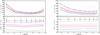 |
Fig. 4 Same as Fig. 3 with triangular configuration with s = 3 Mpc /h, q = 2. |
| In the text | |
Current usage metrics show cumulative count of Article Views (full-text article views including HTML views, PDF and ePub downloads, according to the available data) and Abstracts Views on Vision4Press platform.
Data correspond to usage on the plateform after 2015. The current usage metrics is available 48-96 hours after online publication and is updated daily on week days.
Initial download of the metrics may take a while.