© ESO, 2016

1. Introduction

The decade of 1970s will be remembered as the one in which solar physicists were able to really start to infer the magnetic and thermodynamic properties of the solar plasma from observations. At that time, there was a nice coincidence. On the one hand, the theory of radiative transfer for polarized light was already in its maturity. On the other, computers started to be available for researchers in general and which were powerful enough to carry out complex calculations. It was at this time that the ideas of nonlinear inversion codes were set (Harvey et al. 1972; Auer et al. 1977; Skumanich & Lites 1987).

Inversion algorithms are able to extract information about the magnetic and thermodynamical properties of the solar plasma from the analysis of spectropolarimetric observations. They function by proposing a specific model to explain the observations and then defining a merit function (usually the χ² function, valid under the presence of uncorrelated Gaussian noise). The model parameters are iteratively modified for optimizing the merit function. The first inversion codes were relatively simple and based on strongly simplifying assumptions, like the Milne-Eddington (ME) approximation to analytically solve the radiative transfer equation (e.g., Harvey et al. 1972; Auer et al. 1977; Landi Degl’Innocenti & Landolfi 2004). These inversion codes are still used today, like VFISV (Borrero et al. 2007, 2010), MILOS (Orozco Suárez et al. 2007) or MERLIN (Skumanich & Lites 1987; Lites et al. 2007).

An enormous step forward was introduced by Ruiz Cobo & del Toro Iniesta (1992), who developed Stokes inversion based on response functions (SIR), an inversion code that recovers the optical depth stratification of the physical quantities (temperature, magnetic field, velocity, etc.) from the interpretation of the Stokes profiles. This code is based on the idea of the response function (Landi Degl’Innocenti & Landi Degl’Innocenti 1977), that allows the user to link the perturbation in the emergent Stokes parameters with perturbations in the physical parameters. One of the key ingredients that facilitated the development of these inversion codes was the possibility to find an analytical expression for the response functions in local thermodynamic equilibrium (LTE; Sanchez Almeida 1992; Ruiz Cobo & del Toro Iniesta 1994). Based on the essence of SIR, several nonlinear inversion codes are now available, some of them even dealing with the much more difficult case of the inversion of spectral lines in non-LTE (NICOLE; Socas-Navarro et al. 2000, 2015). All these 1D inversion codes are based on the concept of so-called nodes, that need to be defined a priori. These nodes mark positions along the optical depth axis where the value of the physical parameters will be modified to fit the Stokes profiles. The full stratification of the atmosphere between the nodes, which is needed to accurately integrate the radiative transfer equation and to derive the gas pressure scale, is interpolated using a piece-wise polynomial. The complexity of the solution then critically depends on the number of nodes that are employed to describe each of the physical parameters.

After more than a decade without any fundamental improvement (except perhaps the introduction of Bayesian inference into the field; Asensio Ramos et al. 2007, 2012; Asensio Ramos 2009), we are now going through another interesting era, again driven by the improvements in computational power. On the one hand, van Noort (2012) has developed a spatially coupled two-dimensional inversion code in which the effect of the telescope point spread function (PSF) is taken into account. The PSF couples nearby pixels so that deconvolution and inversion is done at the same time. On the other hand, following a similar motivation, Ruiz Cobo & Asensio Ramos (2013) have used a regularized deconvolution of the Stokes profiles based on the principal component analysis (PCA) and have used SIR to invert the deconvolved Stokes parameters.

Fig. 1 Examples of situations in which systematic effects are important when extracting information from spectral lines.

Arguably, the last step in the evolution of inversion codes has been the introduction of regularization ideas based on the concept of sparsity or compressibility¹ (e.g., Starck et al. 2010). Asensio Ramos & de la Cruz Rodríguez (2015) have presented an inversion code for the inversion of Stokes profiles that uses ℓ₀ or ℓ₁ regularization on a transformed space². The two-dimensional maps of parameters are linearly transformed (Fourier, wavelet, or any other appropriate transformation can be used) and assumed to be sparse in the transformed domain. This introduces two important constraints. First, the sparsity assumption reduces the number of unknowns in the problem, avoiding overfitting. Second, the global character of the transformations that are routinely used, spatial correlation of the result is automatically taken into account. Consequently, the Stokes parameters observed at every pixel potentially introduces constraints onto every other pixel of the observed map. This is the first time that the inherent spatial correlation of the physical parameters has been taken into account in inversion codes. This results in much more stable inversion codes that do not produce spurious pixel-by-pixel variations of the maps of physical quantities. Additionally, the complexity of the solution is automatically adapted, producing more structure where it is needed.

In the conclusions of Asensio Ramos & de la Cruz Rodríguez (2015), we point out that the sparsity regularization can be applied to invert Stokes profiles with systematic effects. This is precisely what we present in this paper. A customary way of dealing with systematic effects in current inversions is to downweight the influence on the merit function of the parts of the spectrum that are affected by these effects. Although it works in practice, it depends on a set of parameters (e.g., region and factor of the downweighting), which make it quite subjective. Instead, we propose several basis sets (orthogonal and non-orthogonal) to absorb the systematic effects (for instance, telluric lines) in the Stokes profiles and use a proximal projection algorithm (e.g., Parikh & Boyd 2014) to make the solution automatically adapt to the necessary complexity. We show that the modifications needed in existing inversion codes are minimal so that this approach can be introduced without much effort.

2. Sparsity regularization

Our objective is to fit the observed Stokes parameters, which are discretized at N finite wavelength points λ_j. For simplicity, we stack the four Stokes parameters in a long vector of length 4N so that O = [I(λ₁),...,I(λ_N),Q(λ₁),...,U(λ₁),...,V(λ₁),...,V(λ_N)] ^† (with † the transpose). The fit is carried out using a model atmosphere, with the aim of extracting useful thermal, dynamic, and magnetic information from them. Additionally, we make the assumption that these Stokes parameters are perturbed by some uncontrollable systematic effects. These systematic effects can be, for instance, telluric lines produced by absorption in the Earth atmosphere, variations along the spectral direction produced by an incorrect illumination of the camera or a low-quality flatfielding, etc. Examples of these situations are found in Fig. 1. The left panel shows the well-known region around 6302 Å  that contains two Fe i lines, which are blended with two telluric lines. This is of special importance for the Fe i line at 6302.5 Å. Extracting physical information from the line requires then to avoid the far wings, which can lead to problems in the deepest parts of the atmosphere. The right panel shows the region around 10 830 Å, containing an He i multiplet used for chromospheric diagnostics, which is blended with a photospheric Si i line and a telluric line. The interpretation of the He i multiplet, given that it forms on the extended wings of the Si i line, usually requires a previous analysis of the photospheric line. Additionally, the strong chromospheric dynamics induces that the He i multiplet sometimes blends with the telluric absorption.

In very general terms, we can explain the observations with the following generative model: ${O}\mathrm{=}{{S}}_{\mathrm{atm}}\mathrm{\left(}{q}\mathrm{\right)}\mathrm{+}{D}{\alpha }\mathrm{+}{ϵ}\mathit{,}$(1)where α is a vector of dimension d that describes the systematic effects via a dictionary D ∈ R^{4N × d}, also known as synthesis operator. We recall that a dictionary is just a collection of (possibly non-orthogonal) functions that are used to describe the systematic effects. The contribution S_atm(q) contains the Stokes parameters that emerge from a model atmosphere, which depends on a vector of model parameters q, ordered like in O. The noise components ϵ are considered to be Gaussian random variables with zero mean and diagonal covariance matrix. We note that when the size of the dictionary equals the number of observed spectral points (d = 4N) and D = 1 (with 1 the identity matrix), the model for the systematic effects described in Eq. (1) turns out to be very flexible because α refers to the particular value of the systematic effects at each sampled wavelength point.

From this generative model, the merit function that has to be optimized is the χ² with diagonal covariance, in our case given by ${\mathit{\chi }}_{{D}}^{\mathrm{2}}\mathrm{\left(}{q}\mathit{,}{\alpha }\mathrm{\right)}\mathrm{=}\frac{\mathrm{1}}{\mathrm{4}\mathit{N}}\sum _{\mathit{j}\mathrm{=}\mathrm{1}}^{\mathrm{4}\mathit{N}}{\mathit{w}}_{\mathit{j}}\frac{{\mathrm{\left[}{\mathit{S}}_{\mathrm{atm}\mathit{,j}}\mathrm{\right(}{q}\mathrm{)}\mathrm{+}\mathrm{(}{D}{\alpha }{\mathrm{)}}_{\mathit{j}}\mathrm{-}{\mathit{O}}_{\mathit{j}}\mathrm{]}}^{\mathrm{2}}}{{\mathit{\sigma }}_{\mathit{j}}^{\mathrm{2}}}\mathit{,}$(2)where we make explicit the dependence of the merit function on the election of the dictionary. The previous merit function considers a potentially different noise variance ${\mathit{\sigma }}_{\mathit{j}}^{\mathrm{2}}$ for every Stokes parameter and wavelength position, which is surely the case for very strong lines in which the number of photons in the core is much more absorbed than the wings. Additionally, it is customary to introduce weights w_j for each Stokes parameter to increase the sensitivity to some parameters when carrying out the inversion³. These weights are precisely the ones that are currently used to deal with systematic effects, by decreasing their values for specific wavelength points.

The inferred physical parameters are typically found by solving the following maximum-likelihood problem: ${\arg \hspace{0.17em}\min }_{{q,}{\alpha }}\hspace{0.17em}{\mathit{\chi }}_{{D}}^{\mathrm{2}}\mathrm{\left(}{q}\mathit{,}{\alpha }\mathrm{\right)}\mathit{,}$(3)where the operator arg min returns the value of q and α that minimizes the ${\mathit{\chi }}_{{D}}^{\mathrm{2}}\mathrm{\left(}{q}\mathit{,}{\alpha }\mathrm{\right)}$ function. We note that Eq. (3) is, in general, non-convex⁴ for the inversion of Stokes parameters. Therefore, we only aspire to reach one of the local minima and later check for the physical relevance of the solution. Problem 3 is usually solved by a direct application of the Levenberg-Marquardt (LM) algorithm (Levenberg 1944; Marquardt 1963), which is especially suited to the optimization of these types of ℓ₂-norms. Although Problem 3 is stated without any constraint, it is clear from the introduction that it is customary to regularize the solution by imposing some regularity of the solution through the use of nodes. Consequently, the vector of parameters q contains the value of the physical parameters (temperature, magnetic field, velocity etc.) at a small number of depths in optical depth in the atmosphere. In between these points, the physical properties are interpolated from the values at these nodes.

Without any additional constraint for α, it is clear that we will encounter cross-talk between α and q. The fundamental reason is that our regressor for the systematic effects is so flexible that it can potentially fit the observations perfectly, including the specific noise realization. As noted above, if d = 4N and D = 1, a solution to Eq. (3) is α = O and S_atm(q) = 0 for every observed wavelength. This trivial solution is of no interest because it does not extract any relevant physical information from the observations. To overcome this possibility, we follow recent ideas (Candès et al. 2006; Starck et al. 2010; Asensio Ramos & de la Cruz Rodríguez 2015) and regularize the problem by imposing a sparsity constraint on α or, in general, on any transformation of α. Two fundamental approaches to include this sparsity penalty have been proposed (Starck et al. 2010). Each one has advantages and disadvantages, as we will show in Sect. 4.

2.1. The analysis penalty approach

This approach is based on having as many degrees of freedom as observed data points (d = 4N) and D = 1 and solving the following problem: ${\arg \hspace{0.17em}\min }_{{q,}{\alpha }}\hspace{0.17em}{\mathit{\chi }}_{{1}}^{\mathrm{2}}\mathrm{\left(}{q}\mathit{,}{\alpha }\mathrm{\right)}\mathit{,}\hspace{0.17em}\hspace{0.17em}\mathrm{subject}\hspace{0.17em}\mathrm{to}\hspace{0.17em}\mathrm{\parallel }{W}{\alpha }{\mathrm{\parallel }}_{\mathit{p}}\mathrm{\le }\mathit{s,}$(4)where W is the matrix associated with any linear transformation of interest, either orthogonal or not, while s is a predefined threshold. We also reiterate that ∥ x ∥ _p = ( ∑ _i | x_i | ^p)^{1 /p} is the ℓ_q-norm. For instance, the ℓ₀ norm of a vector is just the number of non-zero elements, while the ℓ₁ norm is the sum of the absolute value of its elements. In other words, solving Eq. (4) requires us to seek the pair (q,α) that better fits our observations, which imposes that the projection of the systematic effects on the transformed domain defined by W is sparse. The so-called analysis penalty comes from the fact that W is the analysis operator, which carries the vector α to the transformed sparsity-inducing domain (Elad et al. 2007; Starck et al. 2010). It is especially suited to deal with cases in which W is non-orthogonal and/or overcomplete.

The solution to the previous problem when p = 0 (or equivalently when p = 1 under some conditions; Candès et al. 2006; Donoho 2006) is known to coincide with the exact solution when it exists. Sparsity is, therefore, a very convenient regularization. The only degree of freedom is to find the appropriate transformation W. The same problem can be written equivalently with the addition of a regularization parameter (λ): ${\arg \hspace{0.17em}\min }_{{q,}{\alpha }}\hspace{0.17em}\left[\frac{\mathrm{1}}{\mathrm{4}\mathit{N}}\sum _{\mathit{j}\mathrm{=}\mathrm{1}}^{\mathrm{4}\mathit{N}}{\mathit{w}}_{\mathit{j}}\frac{{\mathrm{\left[}{\mathit{S}}_{\mathrm{atm}\mathit{,j}}\mathrm{\right(}{q}\mathrm{)}\mathrm{+}{\mathit{\alpha }}_{\mathit{j}}\mathrm{-}{\mathit{O}}_{\mathit{j}}\mathrm{]}}^{\mathrm{2}}}{{\mathit{\sigma }}_{\mathit{j}}^{\mathrm{2}}}\mathrm{+}\mathit{\lambda }\mathrm{\parallel }{W}{\alpha }{\mathrm{\parallel }}_{\mathit{p}}\right]\mathit{.}$(5)

2.2. The synthesis penalty approach

This approach is based on having D = W^T and imposing a sparsity constraint on the α vector itself. Consequently, we have to solve the problem ${\arg \hspace{0.17em}\min }_{{q,}{\alpha }}\hspace{0.17em}{\mathit{\chi }}_{{{W}}^{\mathrm{T}}}^{\mathrm{2}}\mathrm{\left(}{q}\mathit{,}{\alpha }\mathrm{\right)}\mathit{,}\hspace{0.17em}\hspace{0.17em}\mathrm{subject}\hspace{0.17em}\mathrm{to}\hspace{0.17em}\mathrm{\parallel }{\alpha }{\mathrm{\parallel }}_{\mathit{p}}\mathrm{\le }\mathit{s,}$(6)which, in Lagrangian form, becomes ${\arg \hspace{0.17em}\min }_{{q,}{\alpha }}\hspace{0.17em}\left[\frac{\mathrm{1}}{\mathrm{4}\mathit{N}}\sum _{\mathit{j}\mathrm{=}\mathrm{1}}^{\mathrm{4}\mathit{N}}{\mathit{w}}_{\mathit{j}}\frac{{\mathrm{\left[}{\mathit{S}}_{\mathrm{atm}\mathit{,j}}\mathrm{\right(}{q}\mathrm{)}\mathrm{+}\mathrm{(}{{W}}^{\mathrm{T}}{\alpha }{\mathrm{)}}_{\mathit{j}}\mathrm{-}{\mathit{O}}_{\mathit{j}}\mathrm{]}}^{\mathrm{2}}}{{\mathit{\sigma }}_{\mathit{j}}^{\mathrm{2}}}\mathrm{+}\mathit{\lambda }\mathrm{\parallel }{\alpha }{\mathrm{\parallel }}_{\mathit{p}}\right]\mathit{.}$(7)The name synthesis penalty comes from the fact that W^T is the synthesis operator, which generates the systematic effects from the vector α living on the sparsity-inducing transformed domain.

Elad et al. (2007) note that both approaches are equivalent when W is an orthogonal transform (like Fourier, wavelet, etc.), because it fulfills W^TW = 1. However, they solve completely different problems when W is non-orthogonal.

2.3. Transformations

In this paper, we consider three options for the regularization term. The first one uses as regularization an orthogonal wavelet transform. The fact that W is orthogonal will slightly simplify the algorithms. The second one is a non-orthogonal overcomplete isotropic undecimated wavelet transform using the B₃-spline (Starck et al. 2010). Finally, we will use a hand-made non-orthogonal transform made of Voigt functions centered at specific locations in the spectrum, which will be used to absorb the systematic effects. We defer the detailed description of each one until Sect. 3.3.

3. The proposed optimization

Given the special structure of both problems defined in Eqs. (5) and (7), in which the regularization only occurs for the α variables, we propose to use an alternating optimization method. If α is fixed, Eq. (5) becomes the traditional least-squares problem for q, which is solved efficiently with Newton-type methods like the Levenberg-Marquardt algorithm. This method uses second-order information given by H_q, the Hessian of the merit function with respect to the q variables: ${{q}}_{\mathit{i}\mathrm{+}\mathrm{1}}\mathrm{=}{{q}}_{\mathit{i}}\mathrm{-}{Ĥ}\begin{array}{c}-1\\ \mathit{q}\end{array}{\mathrm{\nabla }}_{\mathit{q}}{\mathit{\chi }}_{{1}}^{\mathrm{2}}\mathrm{\left(}{{q}}_{\mathit{i}}\mathit{,}{\alpha }\mathit{i}\mathrm{\right)}\mathit{,} \hspace{0.17em}\hspace{0.17em}\hspace{0.17em} \mathrm{with}{\alpha }\mathit{i}\mathrm{fixed}\mathit{.}$(8)Conforming to the prescriptions of the Levenberg-Marquardt algorithm, we use a modified Hessian matrix by enhancing its diagonal by a factor β, so that Ĥ_q = H_q + βdiag(H_q). This hyperparameter is modified during the iteration to shift between the gradient descent method (large β) and Newton-type method (small β). We note that inverting the Hessian matrix with a truncated singular value decomposition (Ruiz Cobo & del Toro Iniesta 1992) introduces an extra regularization on the physical parameters at the nodes that is often needed.

3.1. The analysis penalty

On the other hand, when q is fixed, Eq. (5) becomes a standard sparsity-constrained linear problem for α. This problem can be solved efficiently using proximal algorithms (Parikh & Boyd 2014; Asensio Ramos & de la Cruz Rodríguez 2015), which are especially suited to solving problems of the type:${\arg \hspace{0.17em}\min }_{{\alpha }}\mathit{f}\mathrm{\left(}{\alpha }\mathrm{\right)}\mathrm{:}\mathrm{=}\mathit{g}\mathrm{\left(}{\alpha }\mathrm{\right)}\mathrm{+}\mathit{h}\mathrm{\left(}{\alpha }\mathrm{\right)}\mathit{,}$(9)where $\mathit{g}\mathrm{\left(}{\alpha }\mathrm{\right)}\mathrm{=}{\mathit{\chi }}_{{1}}^{\mathrm{2}}\mathrm{\left(}{q}\mathit{,}{\alpha }\mathrm{\right)}$, is a smooth function and h(α) = λ ∥ Wα ∥ _p is a convex but not necessarily smooth function (we note that the derivative of the ∥ Wα ∥ _p term is not continuous). We propose the following first-order iterative scheme to solve the problem: ${\alpha }\mathit{i}\mathrm{+}\mathrm{1}\mathrm{=}{\mathrm{prox}}_{\mathit{p,\lambda ,}{W}}\mathrm{[}{\alpha }\mathit{i}\mathrm{-}\mathit{\tau }{\mathrm{\nabla }}_{\mathit{\alpha }}{\mathit{\chi }}_{{1}}^{\mathrm{2}}\mathrm{(}{{q}}_{\mathit{i}\mathrm{+}\mathrm{1}}\mathit{,}{\alpha }\mathit{i}{\mathrm{\left)}}^{\mathrm{\right]}} \mathrm{with}{{q}}_{\mathit{i}\mathrm{+}\mathrm{1}}\mathrm{fixed}\mathit{,}$(10)where the operator prox_p,λ,W is the proximal projection operator (Parikh & Boyd 2014) associated with the constraint ∥ Wα ∥ _p, which we show how to efficiently compute in Sect. 4. The election of the step size τ is important for the convergence of the algorithm. This is known to converge, provided the step size fulfills τ< 2 / ∥ H_α ∥ ², where ∥ H_α ∥ is the spectral norm of the Hessian of the merit function with respect to α (given by the square root of the maximum eigenvalue of ${{H}}_{\mathit{\alpha }}^{\mathrm{T}}{{H}}_{\mathit{\alpha }}$). We note that faster algorithms like FISTA (Beck & Teboulle 2009; Asensio Ramos & de la Cruz Rodríguez 2015) can also be used.

Given the simple dependence of ${\mathit{\chi }}_{{q}\mathit{,}{\alpha }}^{\mathrm{2}}$ on α, it can be proven (e.g., Starck et al. 2010) that Eq. (10) can be simplified to finally obtain: ${\alpha }\mathit{i}\mathrm{+}\mathrm{1}\mathrm{=}{\mathrm{prox}}_{\mathit{p,\lambda ,}{W}}\left[{{S}}_{\mathrm{atm}}\mathrm{\left(}{{q}}_{\mathit{i}\mathrm{+}\mathrm{1}}\mathrm{\right)}\mathrm{-}{O}\right] \mathrm{with}{{q}}_{\mathit{i}\mathrm{+}\mathrm{1}}\mathrm{fixed}\mathit{.}$(11)In other words, the estimation of the systematic effects for a new iteration is very simple and reduces to computing the proximal projection of the residual between the observed Stokes profiles and the current modeled ones. We think that this approach provides a very transparent and intuitive understanding of what the algorithm is doing. We note that the best results have been found applying Eq. (11) every ~ 3 iterations of the LM algorithm.

3.2. The synthesis penalty

When q is fixed, Eq. (7) again becomes a sparsity-constrained problem for α. In this case, the sparsity penalty h(α) = ∥ α ∥ _p is much simpler, but the function $\mathit{g}\mathrm{\left(}{\alpha }\mathrm{\right)}\mathrm{=}{\mathit{\chi }}_{{{W}}^{\mathrm{T}}}^{\mathrm{2}}\mathrm{\left(}{q}\mathit{,}{\alpha }\mathrm{\right)}$ is more complex because of the presence of the synthesis operator W^T. We propose solving the problem using the following first-order iterative scheme: ${\alpha }\mathit{i}\mathrm{+}\mathrm{1}\mathrm{=}{\mathrm{prox}}_{\mathit{p,\lambda ,\tau }}\mathrm{[}{\alpha }\mathit{i}\mathrm{-}\mathit{\tau }{\mathrm{\nabla }}_{\mathit{\alpha }}{\mathit{\chi }}_{{{W}}^{\mathrm{T}}}^{\mathrm{2}}\mathrm{(}{{q}}_{\mathit{i}\mathrm{+}\mathrm{1}}\mathit{,}{\alpha }\mathit{i}{\mathrm{\left)}}^{\mathrm{\right]}} \mathrm{with}{{q}}_{\mathit{i}\mathrm{+}\mathrm{1}}\mathrm{fixed}\mathit{,}$(12)where τ< 2 / ∥ H_α ∥ ², which can be computed from the spectral norm of the transformation matrix W, and the proximal operator prox_p,λ,τ is described in the following. We point out that a more complex second-order iterative scheme is discussed in the Appendix.

3.3. Computing the proximal operators

The previous iterative schemes rely on the existence of algorithms for the computation of the proximal projection operators prox_p,λ,τ(α) and prox_p,λ,W(α).

3.3.1. Computing prox_p,λ,τ(α)

This operator is very simple to compute for typical choices of p (Parikh & Boyd 2014). Useful cases of the regularization term are the ℓ₀-norm (p = 0) or the ℓ₁-norm (p = 1). In the case of the ℓ₀-norm, the proximal operator reduces to the hard-thresholding operator, which is trivially given by ${\mathrm{prox}}_{\mathit{p}\mathrm{=}\mathrm{0}\mathit{,\lambda ,\tau }}\mathrm{\left(}{\alpha }\mathrm{\right)}\mathrm{=}\{\begin{array}{c}\\ & \mathrm{\left|}{\alpha }\mathrm{\right|}\mathit{>}\mathit{\tau \lambda }\\ & \mathrm{otherwise}\mathit{.}\end{array}$(13)where τ is the step-size defined in Sect. 3.1 and λ is the regularization parameter that we introduced in Eq. (5). For the ℓ₁-norm, it reduces to the soft-thresholding operator, which is given by ${\mathrm{prox}}_{\mathit{p}\mathrm{=}\mathrm{1}\mathit{\lambda ,\tau }}\mathrm{\left(}{\alpha }\mathrm{\right)}\mathrm{=}\mathrm{sign}\mathrm{\left(}{\alpha }\mathrm{\right)}\mathrm{\left(}\mathrm{\right|}{\alpha }\mathrm{|}\mathrm{-}\mathit{\tau \lambda }{\mathrm{)}}_{\mathrm{+}}\mathit{,}$(14)where (·)₊ denotes the positive part. Other proximal operators with analytical expressions can be found in Parikh & Boyd (2014).

3.3.2. Computing prox_p,λ,W(α)

The solution of Eq. (11) for any W, either orthogonal or not, is slightly more complicated and requires some elements of proximal calculus (Parikh & Boyd 2014). A general algorithm for the solution of the proximal projection of Eq. (11) has been developed by Fadili & Starck (2009), which we reproduce in Alg. 1 for completeness. We note that the algorithm is just a simple iterative scheme that has been proven to converge with the solution, provided the step size τ< 2 / ∥ W ∥ ².

It is interesting to note that when W is an orthogonal transform, Alg. 1 hugely simplifies and the solution to Eq. (11) can be obtained with (Starck et al. 2010): ${\alpha }\mathrm{=}{{W}}^{\mathrm{T}}\mathrm{[}{\mathrm{prox}}_{\mathit{p,\lambda ,\tau }}{\mathrm{\left(}{W}{\alpha }\mathrm{\right)}}^{\mathrm{]}}\mathit{.}$(15)In other words, the vector α is first transformed, then it is thresholded using the appropriate proximal operator, and finally transformed back to the original domain. If the transformation is unitary, so that W^TW = 1, the result of the application of Eq. (15) leaves the value of α unchanged for λ = 0.

Another interesting use of Eq. (15) is that it is equivalent to the first iteration of Alg. 1. We carry out experiments in the following sections to verify if using this simple approximation in the general case of non-orthogonal W gives good results.

3.4. Selection of λ

As we show in the next section, λ has a strong impact on the sparsity of the final solution. When λ is too small, overfitting clearly appears. On the contrary, if λ is large, the fit is typically of bad quality. Therefore, the selection of λ requires some fine-tuning, but it is possible to have an order of magnitude estimation using very simple arguments. As noted in Eqs. (13) and (14), the thresholding happens for values of the α parameters that are larger than τλ. Therefore, if we want to avoid values of α that are smaller than η, then λ ~ η ∥ W ∥ ². For the orthogonal unitary transforms, we find that the spectral norm is ∥ W ∥ = 1.

3.5. Summary

The full step-by-step algorithms are described in Algs. 2 and 3, together with Alg. 1 for the application of the proximal operator described in step 4 of Alg. 2. We want to clarify to any potential user of this method that the only real difference between current inversion codes for the Stokes parameters and our approach is in point 4 of Alg. 2, together with the necessity to include the systematic effects in the calculation of the gradient and Hessian with respect to the q variables. This step is very easy to carry out and can be implemented in any existing inversion code with only a few lines of programming.

4. Examples

In this section we demonstrate the capabilities of Algs. 2 and 3 in the inversion of Stokes profiles using several transformation matrices W and two datasets. For simplicity and for the purpose of clarity, we only focus on Stokes I, for which the systematic effects are usually more important. Throughout this section, we use the ℓ₀-norm as regularization, so we apply the proximal operator of Eq. (13). The codes used in this paper can be obtained online⁵.

4.1. Observations

To show examples of application, we choose two spectral regions of special interest that suffer from the problems described in this paper. The first one is the region around 10 830 Å, which contains the He i multiplet at 10 830 Å and is displayed in the right panel of Fig. 1. This multiplet is used for diagnosing the magnetic properties of chromospheric material. Owing to the potentially large Doppler shifts in the chromosphere (e.g., Lagg et al. 2007), it is interesting to apply our approach to this multiplet.

The observations that we analyze were obtained with the Vacuum Tower Telescope (VTT) on the Observatorio del Teide with the TIP-II instrument (Collados et al. 2007). The profiles were extracted from a plage region close to a pore. The He i multiplet is synthesized with the help of hazel (Asensio Ramos et al. 2008), which gives the S_atm(q) part of Eq. (1). The spectral lines are characterized by the optical depth on the red component of the multiplet Δτ, the Doppler broadening of the line v_th, and the bulk velocity of the plasma v.

The second region is the well-known region around 6301−6302 Å that contains an Fe i doublet. This region also contains two telluric absorptions. The Stokes profiles, shown in the left panel of Fig. 1, have been obtained from the ground with the POlarimetric LIttrow Spectrograph (POLIS; Beck et al. 2005) and belong to the observations of the quiet Sun analyzed by Martínez González et al. (2008).

To fit the profiles, we choose an atmosphere in LTE and we infer the depth stratification of the temperature, velocity along the line-of-sight, and microturbulent velocity. For this experiment, we fix the number of nodes of the parameterization: five nodes for the temperature, three for the bulk velocity and one for the microturbulent velocity. Like virtually all inversion codes with depth stratification (e.g., Ruiz Cobo & del Toro Iniesta 1992), we place the nodes equispaced in the log τ_c axis, with τ_c the continuum optical depth at 5000 Å.

Fig. 2 Left panels: observed (blue) and fitted (green) Stokes I profile for different values of the regularization parameters λ and using an orthogonal wavelet transform as the sparsity-inducing transformation. The dashed red curve shows the inferred systematic effects. The spectral range corresponds to that around the He i multiplet at 10 830 Å. Right panels: first 100 active wavelet coefficients of the set of 512 total coefficients. The percentage of active functions is shown in each panel.

4.2. Orthogonal wavelet regularization

The orthogonal wavelet transform (Jensen & la Cour-Harbo 2001) is a very powerful sparsity-inducing transformation in cases in which the signal is smooth. One of the advantages of the orthogonal wavelet transform is that a fast algorithm to compute the direct and inverse transformation exists, without ever computing the transformation matrix W.

Fig. 3 Observed (blue), fitted (green) and systematic effects (dashed red) obtained using the IUWT in the region around 10 830 Å and using the updated version of hazel. The left panels correspond to using the full Alg. 1, while the right panel shows the results when using the simplified Eq. (15).

The specific approach for orthogonal transformations is irrelevant because both the analysis and synthesis penalties are equivalent. For convenience, we choose to do this study under the analysis penalty case. We impose the sparsity constraint using the transformation matrix W associated with the Daubechies-8 orthogonal wavelet and for different values of the regularization parameter λ. The results are shown in Fig. 2. The left panel displays the observed data, the final fit (including systematic effects) and the inferred systematic effects. The right panel shows the wavelet coefficients of the systematic effects, showing only the first 100 coefficients of the potential 512 coefficients (the wavelength axis contains 512 sampled points). Each panel contains the percentage of active (non-zero) wavelet coefficients. We note that the fit quality is strongly affected by the value of the regularization parameters λ. The important point is that it is possible to find values of λ that lead to a good fit of the He i multiplet and simultaneously fit the systematic effects. Of special relevance, in this case, is the extended wing of the Si i, which sometimes makes it difficult to set a continuum level for the 10 830 Å multiplet. Using this approach, the continuum level is automatically obtained from the fit.

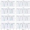Fig. 4 Observed (blue), fitted (green), and systematic effects (dashed red) obtained using the IUWT in the 6301−6302 Å spectral region and using the inversion code that assumes local thermodynamic equilibrium. The left panels correspond to using the full Alg. 1, while the right panel shows the results when using the simplified Eq. (15).

When λ is small, a significant overfitting of the data occurs, in which even the noise is absorbed by the systematic effects. For very large λ, the method cannot fit the observations. For intermediate values of λ, a very nice fit is obtained. The optimal thresholding of the wavelet coefficients is similar to the expected noise level, as pointed out by Starck et al. (2010). Using only 10% of the wavelet coefficients is probably enough to have a fit of the whole spectral region. It is interesting that the model that we impose for the He i multiplet is probably not enough to explain the observations at the noise level. This is the reason why some “extra absorption” is added by the systematic effects to the wings of the red component. If this behavior is undesirable, it is potentially possible to introduce an extra regularization to avoid them (for instance, an additional ℓ₀ or ℓ₁ regularization for the vector α). However, we demonstrate in the following that a better option is to regularize using different W transformations.

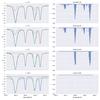Fig. 5 Observed (blue) and fitted (green) Stokes I profile for different values of the regularization parameters λ and using a dictionary made of Voigt functions centered at every pixel. The dashed red curve shows the inferred systematic effects. The left panels show the results for the Fe i lines, while the right panels show the active functions, with the label indicating the percentage of active functions.

4.3. Isotropic undecimated wavelet regularization

The isotropic undecimated wavelet transform (IUWT; Starck & Murtagh 1994; Starck et al. 2010) algorithm is a non-orthogonal redundant multiscale transform that is well suited to objects that are more or less isotropic. This transform has found great success for the denoising of astronomical images (e.g., Starck et al. 2010, and references therein). Recently, we have witnessed examples of applications to one-dimensional spectra (Machado et al. 2013). Given that this is a redundant non-orthogonal transform, the analysis penalty approach is more efficient from a computational point of view.

The IUWT can be efficiently applied using the à-trousalgorithm, which proceeds as follows: The original data I(λ) are filtered, in our case using the B₃-spline given by the filter [1,4,6,4,1] / 16. The filtered data are substracted from the original ones, obtaining what is commonly known as the detail, w_i(λ). The filtered data are again iteratively filtered (with scaled filters) up to a depth d, computing the detail in each scale. The final smoothed signal will be termed c_d(λ). At the end, we have a smoothed version of the original signal and a set of details at each depth. The size of the IUWT is d + 1 times the original data, so the information is really encoded on the correlation among the transformed coefficients. The data are reconstructed from the transformed data simply using$\mathit{I}\mathrm{\left(}\mathit{\lambda }\mathrm{\right)}\mathrm{=}{\mathit{c}}_{\mathit{d}}\mathrm{\left(}\mathit{\lambda }\mathrm{\right)}\mathrm{+}\sum _{\mathit{i}\mathrm{=}\mathrm{1}}^{\mathit{d}}{\mathit{w}}_{\mathit{i}}\mathrm{\left(}\mathit{\lambda }\mathrm{\right)}\mathit{.}$(16)The results shown in Fig. 3 for the He i multiplet and Fig. 4for the Fe i doublet have been obtained using the IUWT up to d = 6 and applying the hard thresholding operator to all the details. The left panel shows the results when the full Alg. 1is used to apply the proximal algorithm, while the right panels give the result when only the first iteration of this algorithm is used, which corresponds to using Eq. (15). The application of Eq. (15) cannot assure convergence to the correct solution to the problem, but we have tested that it does a very good job. This simplifies the application of our proposed algorithm to any existing inversion code because Eq. (15) can be implemented in only one or a few lines of code.

When the value of λ is small, we witness the overfitting again, which also includes the addition of some broadening of the red component of the He i. When λ is large, the fit is of low quality. In the intermediate range close to the expected noise standard deviation, we find an excellent fit of the whole profile, with a flat contribution exactly where the He i multiplet is located.

It is interesting to note that we have empirically found that applying Eq. (15) instead of solving the full problem via Alg. 1 gives better and more robust results (see Figs. 3 and 4). The reason has to be due to the fact that we are solving the optimization problem of Eqs. (5) or (7) by separating it into two simpler problems via an alternating optimization method. It is a general characteristic of these methods that they work better in practice if none of the two problems is solved with full precision at each iteration, but only approximately. If any of the two problems is solved with precision in any iteration, one can produce some amount of overfitting that is very difficult to compensate for in later iterations.

4.4. Voigt functions

The final example uses another non-orthogonal and redundant transformation, in this case not of general applicability, but tailored to explain the systematic effects. The Hermite functions described by del Toro Iniesta & López Ariste (2003) is a good option, but we prefer to utilize a basis set made of Voigt functions centered at every sampled wavelength point: ${\mathit{\phi }}_{\mathit{i}}\mathrm{\left(}\mathit{\lambda }\mathrm{\right)}\mathrm{=}\mathit{H}\left(\frac{\mathit{\lambda }\mathrm{-}{\mathit{\lambda }}_{\mathit{i}}}{\mathrm{\Delta }}\mathit{,a}\right)\mathit{.}$(17)Even though the basis is non-orthogonal, it is much easier in this case to work in the synthesis prior approach, because the results are much more transparent. The reason is that we directly impose the sparsity constraint on the coefficients associated with all the Voigt functions.

In this case, we focus on the 6301−6302 Å spectral region. The systematic effects are modeled with Voigt functions placed at every sampled wavelength between 6301.15 and 6302.93 Å, which includes both Fe i lines and both telluric contaminations. The damping constant is fixed to a = 0.8, which gives line wings similar to those observed in the telluric lines. To boost sparsity, we consider two different widths, Δ = 14.8,29.6 mÅ, although more fits and damping parameters can be easily considered with ease.

The results are displayed in Fig. 5 for different values of λ. The left panel shows the observations and the fit, together with the inferred systematic effects. The right panel shows the active Voigt functions. When λ is too small, a very good fitting is found, but we can see that the optimization induces corrections on the spectral lines of interest. This is, in principle, undesired, although it is clearly stating that the model proposed for the spectral lines cannot fit them with enough precision. When λ is large, the fit of the systematic effects is bad, which negatively impacts the fit of the spectral lines of interest. For intermediate values of the regularization parameter, we find an acceptable fit, where only the telluric absorption lines are fitted by the systematic effects with a very sparse solution.

5. Conclusions

In this study, we have developed a new method that enables systematic effects to be dealt with in data inversions. These systematic effects can include a variety of calibration defects, spectral lines from the Earth’s atmosphere, or spectral features that are present in the observations that our model atmosphere cannot reproduce. Our method builds upon the assumption that these systematic effects are not random noise and, therefore, they have an inherent level of sparsity in a suitable basis set.

We have shown that the assumption of sparsity induces a very powerful regularization because the resulting cross-talk between the inversion model and the systematic effects can be made very low. To do so, we have introduced a regularization parameter λ that must be adjusted according to the needs of each problem based on experience. However, we argue that this step is not very different from selecting the weights of the observations in current implementations of inversion codes and a rough estimate can be obtained a priori.

Although the mathematical characterization of the algorithm can appear a bit convoluted and depends on recent advances on the optimization of non-smooth functions, a few extra lines of code should suffice to make it work with current inversion codes. Our experience with the SIR and Hazel codes has positively confirmed this. When these systematic effects are not corrected, inversion codes usually try to overcompensate their effect by converging the parameters of the model to a wrong solution. Our method minimizes the impact of such effects in the convergence of the solution when an adequate value of the regularization parameter is selected.

Our method has a few interesting advantages over the downweighting technique for dealing with systematic effects. Arguably the most important one concerns the assumptions imposed on the generative model. Using the χ² merit function requires that the uncertainty of the residual between the observations and the model is Gaussian with zero mean and a certain variance. This is not true unless one is able to model all expected signals. Only if everything is modeled (to a certain level, of course), can one be sure that the results can be interpreted appropriately (for instance, error bars). A second advantage concerns the reduction in the subjectivity on the election of parameters. One only needs to choose the value of λ and the method automatically adapts the solution to the systematic effects.

Acknowledgments

Financial support by the Spanish Ministry of Economy and Competitiveness through projects AYA2014-60476-P, AYA2014-60833-P, and Consolider-Ingenio 2010 CSD2009-00038 are gratefully acknowledged. J.d.l.C.R. is supported by grants from the Swedish Research Council (Vetenskapsrådet) and the Swedish National Space Board. A.A.R. also acknowledges financial support through the Ramón y Cajal fellowship. This research has made use of NASA’s Astrophysics Data System Bibliographic Services. This article is based on observations taken with the VTT telescope operated on the island of Tenerife by the Kiepenheuer-Institut für Sonnenphysik in the Spanish Observatorio del Teide of the Instituto de Astrofísica de Canarias (IAC). We acknowledge the community effort devoted to the development of the following open-source Python packages that were used in this work: numpy, matplotlib, scipy, seaborn and PyWavelets.

References

Appendix A: Second-order iterative scheme in the synthesis prior

It is possible to use a second-order iterative scheme that would improve over Eq. (12) when using the synthesis prior approach. Instead of a simple step τ, one uses the full Hessian, so that the iterative scheme is updated to read (Lee et al. 2012) $\begin{array}{ccc}{\alpha }\mathit{i}\mathrm{+}\mathrm{1}& \mathrm{=}& {\mathrm{prox}}_{\mathit{p,\lambda }}^{{\mathit{H}}_{\mathit{\alpha }}}\mathrm{[}{\alpha }\mathit{i}\mathrm{-}{{H}}_{\mathit{\alpha }}^{-1}{\mathrm{\nabla }}_{\mathit{\alpha }}{\mathit{\chi }}_{{{W}}^{\mathrm{T}}}^{\mathrm{2}}\mathrm{(}{{q}}_{\mathit{i}\mathrm{+}\mathrm{1}}\mathit{,}{\alpha }\mathit{i}{\mathrm{)}}^{\mathrm{]}} \mathrm{with}{{q}}_{\mathit{i}\mathrm{+}\mathrm{1}}\mathrm{fixed}\mathit{.}\end{array}$(A.1)The main obstacle is the computation of the so-called scaled proximal operator ${\mathrm{prox}}_{\mathit{p,\lambda }}^{{\mathit{H}}_{\mathit{\alpha }}}\mathrm{\left(}{\alpha }\mathrm{\right)}$. It can be demonstrated that this proximal operator can be efficiently computed using the accelerated FISTA iteration (Beck & Teboulle 2009), which is displayed in Alg. 4.

All Figures

	Fig. 1 Examples of situations in which systematic effects are important when extracting information from spectral lines.
In the text

Fig. 2 Left panels: observed (blue) and fitted (green) Stokes I profile for different values of the regularization parameters λ and using an orthogonal wavelet transform as the sparsity-inducing transformation. The dashed red curve shows the inferred systematic effects. The spectral range corresponds to that around the He i multiplet at 10 830 Å. Right panels: first 100 active wavelet coefficients of the set of 512 total coefficients. The percentage of active functions is shown in each panel.

In the text

	Fig. 3 Observed (blue), fitted (green) and systematic effects (dashed red) obtained using the IUWT in the region around 10 830 Å and using the updated version of hazel. The left panels correspond to using the full Alg. 1, while the right panel shows the results when using the simplified Eq. (15).
In the text

	Fig. 4 Observed (blue), fitted (green), and systematic effects (dashed red) obtained using the IUWT in the 6301−6302 Å spectral region and using the inversion code that assumes local thermodynamic equilibrium. The left panels correspond to using the full Alg. 1, while the right panel shows the results when using the simplified Eq. (15).
In the text

Fig. 5 Observed (blue) and fitted (green) Stokes I profile for different values of the regularization parameters λ and using a dictionary made of Voigt functions centered at every pixel. The dashed red curve shows the inferred systematic effects. The left panels show the results for the Fe i lines, while the right panels show the active functions, with the label indicating the percentage of active functions.

In the text

References

- Asensio Ramos, A. 2009, ApJ, 701, 1032 [NASA ADS] [CrossRef] [Google Scholar]
- Asensio Ramos, A., & de la Cruz Rodríguez, J. 2015, A&A, 577, A140 [NASA ADS] [CrossRef] [EDP Sciences] [Google Scholar]
- Asensio Ramos, A., Martínez González, M. J., & Rubiño Martín, J. A. 2007, A&A, 476, 959 [NASA ADS] [CrossRef] [EDP Sciences] [Google Scholar]
- Asensio Ramos, A., Trujillo Bueno, J., & Landi Degl’Innocenti, E. 2008, ApJ, 683, 542 [NASA ADS] [CrossRef] [Google Scholar]
- Asensio Ramos, A., Manso Sainz, R., Martínez González, M. J., et al. 2012, ApJ, 748, 83 [NASA ADS] [CrossRef] [Google Scholar]
- Auer, L. H., House, L. L., & Heasley, J. N. 1977, Sol. Phys., 55, 47 [NASA ADS] [CrossRef] [Google Scholar]
- Beck, A., & Teboulle, M. 2009, SIAM J. Img. Sci., 2, 183 [Google Scholar]
- Beck, C., Schmidt, W., Kentischer, T., & Elmore, D. 2005, A&A, 437, 1159 [NASA ADS] [CrossRef] [EDP Sciences] [Google Scholar]
- Borrero, J. M., Tomczyk, S., Norton, A., et al. 2007, Sol. Phys., 240, 177 [NASA ADS] [CrossRef] [Google Scholar]
- Borrero, J. M., Tomczyk, S., Kubo, M., et al. 2010, Sol. Phys., 35 [Google Scholar]
- Candès, E., Romberg, J., & Tao, T. 2006, Comm. Pure Appl. Math., 59, 1207 [CrossRef] [Google Scholar]
- Collados, M., Lagg, A., Díaz García, J. J., et al. 2007, in The Physics of Chromospheric Plasmas, eds. P. Heinzel, I. Dorotovič, & R. J. Rutten, ASP Conf. Ser., 368, 611 [Google Scholar]
- del Toro Iniesta, J. C., & López Ariste, A. 2003, A&A, 412, 875 [NASA ADS] [CrossRef] [EDP Sciences] [Google Scholar]
- Donoho, D. 2006, IEEE Trans. on Information Theory, 52, 1289 [CrossRef] [Google Scholar]
- Elad, M., Milanfar, P., & Rubinstein, R. 2007, Inverse Problems, 23, 947 [NASA ADS] [CrossRef] [Google Scholar]
- Fadili, M. J., & Starck, J.-L. 2009, in Proc. IEEE International Conference on Image Processing [Google Scholar]
- Harvey, J., Livingston, W., & Slaughter, C. 1972, in Line Formation in the Presence of Magnetic Fields, 227 [Google Scholar]
- Jensen, A., & la Cour-Harbo, A. 2001, Ripples in Mathematics: The Discrete Wavelet Transform (Springer Verlag) [Google Scholar]
- Lagg, A., Woch, J., Solanki, S. K., & Krupp, N. 2007, A&A, 462, 1147 [NASA ADS] [CrossRef] [EDP Sciences] [Google Scholar]
- Landi Degl’Innocenti, E., & Landi Degl’Innocenti, M. 1977, A&A, 56, 111 [NASA ADS] [Google Scholar]
- Landi Degl’Innocenti, E., & Landolfi, M. 2004, Polarization in Spectral Lines (Kluwer Academic Publishers) [Google Scholar]
- Lee, J. D., Sun, Y., & Saunders, M. A. 2012, SIAM J. Opt., 24, 3 [Google Scholar]
- Levenberg, K. 1944, Q. J. Math, 2, 164 [Google Scholar]
- Lites, B., Casini, R., Garcia, J., & Socas-Navarro, H. 2007, Mem. Soc. Astron. It., 78, 148 [NASA ADS] [Google Scholar]
- Machado, D. P., Leonard, A., Starck, J.-L., Abdalla, F. B., & Jouvel, S. 2013, A&A, 560, A83 [NASA ADS] [CrossRef] [EDP Sciences] [Google Scholar]
- Marquardt, D. 1963, SIAM J. Appl. Math., 11, 431 [Google Scholar]
- Martínez González, M. J., Collados, M., Ruiz Cobo, B., & Beck, C. 2008, A&A, 477, 953 [NASA ADS] [CrossRef] [EDP Sciences] [Google Scholar]
- Orozco Suárez, D., Bellot Rubio, L. R., del Toro Iniesta, J. C., et al. 2007,ApJ, 670, 61 [Google Scholar]
- Parikh, N., & Boyd, S. 2014, Foundations and Trends in Optimization, 1 [Google Scholar]
- Ruiz Cobo, B., & Asensio Ramos, A. 2013, A&A, 549, L4 [NASA ADS] [CrossRef] [EDP Sciences] [Google Scholar]
- Ruiz Cobo, B., & del Toro Iniesta, J. C. 1992, ApJ, 398, 375 [NASA ADS] [CrossRef] [Google Scholar]
- Ruiz Cobo, B., & del Toro Iniesta, J. C. 1994, A&A, 283, 129 [NASA ADS] [Google Scholar]
- Sanchez Almeida, J. 1992, Sol. Phys., 137, 1 [NASA ADS] [CrossRef] [Google Scholar]
- Skumanich, A., & Lites, B. W. 1987, ApJ, 322, 473 [Google Scholar]
- Socas-Navarro, H., Trujillo Bueno, J., & Ruiz Cobo, B. 2000, ApJ, 530, 977 [NASA ADS] [CrossRef] [Google Scholar]
- Socas-Navarro, H., de la Cruz Rodriguez, J., Asensio Ramos, A., Trujillo Bueno, J., & Ruiz Cobo, B. 2015, A&A, 577, A7 [NASA ADS] [CrossRef] [EDP Sciences] [Google Scholar]
- Starck, J.-L., & Murtagh, F. 1994, A&A, 288, 342 [NASA ADS] [Google Scholar]
- Starck, J.-L., Murtagh, F., & Fadili, J. M. 2010, Sparse image and signal processing (Cambridge: Cambridge University Press) [Google Scholar]
- van Noort, M. 2012, A&A, 548, A5 [NASA ADS] [CrossRef] [EDP Sciences] [Google Scholar]