| Issue |
A&A
Volume 590, June 2016
|
|
|---|---|---|
| Article Number | A38 | |
| Number of page(s) | 11 | |
| Section | Planets and planetary systems | |
| DOI | https://doi.org/10.1051/0004-6361/201628067 | |
| Published online | 04 May 2016 | |
Four new planets around giant stars and the mass-metallicity correlation of planet-hosting stars⋆
1 Center of Astro-Engineering UC, Pontificia Universidad Católica de Chile, Av. Vicuña Mackenna 4860, 7820436 Macul, Santiago, Chile
e-mail: mjones@aiuc.puc.cl
2 Departamento de Astronomía, Universidad de Chile, Camino El Observatorio 1515, Las Condes, Santiago, Chile
3 Instituto de Astrofísica, Facultad de Física, Pontificia Universidad Católica de Chile, Av. Vicuña Mackenna 4860, 7820436 Macul, Santiago, Chile
4 Millennium Institute of Astrophysics, Santiago, Chile
5 School of Physics and Australian Centre for Astrobiology, University of New South Wales, Sydney, NSW 2052, Australia
6 Departamento de Ciencias Fisicas, Universidad Andres Bello, Avda. Republica 252, Santiago, Chile
7 European Southern Observatory, Casilla 19001, Santiago, Chile
8 Department of Terrestrial Magnetism, Carnegie Institution of Washington, 5241 Broad Branch Road, NW, Washington, DC 20015-1305, USA
9 Key Laboratory of Optical Astronomy, National Astronomical Observatories, Chinese Academy of Sciences, A20 Datun Road, Chaoyang District, 100012 Beijing, PR China
Received: 1 January 2016
Accepted: 10 March 2016
Context. Exoplanet searches have revealed interesting correlations between the stellar properties and the occurrence rate of planets. In particular, different independent surveys have demonstrated that giant planets are preferentially found around metal-rich stars and that their fraction increases with the stellar mass.
Aims. During the past six years we have conducted a radial velocity follow-up program of 166 giant stars to detect substellar companions and to characterize their orbital properties. Using this information, we aim to study the role of the stellar evolution in the orbital parameters of the companions and to unveil possible correlations between the stellar properties and the occurrence rate of giant planets.
Methods. We took multi-epoch spectra using FEROS and CHIRON for all of our targets, from which we computed precision radial velocities and derived atmospheric and physical parameters. Additionally, velocities computed from UCLES spectra are presented here. By studying the periodic radial velocity signals, we detected the presence of several substellar companions.
Results. We present four new planetary systems around the giant stars HIP 8541, HIP 74890, HIP 84056, and HIP 95124. Additionally, we study the correlation between the occurrence rate of giant planets with the stellar mass and metallicity of our targets. We find that giant planets are more frequent around metal-rich stars, reaching a peak in the detection of f = 16.7+15.5-5.9% around stars with [Fe/H] ~ 0.35 dex. Similarly, we observe a positive correlation of the planet occurrence rate with the stellar mass, between M⋆ ~ 1.0 and 2.1 M⊙, with a maximum of f = 13.0+10.1-4.2% at M⋆ = 2.1 M⊙.
Conclusions. We conclude that giant planets are preferentially formed around metal-rich stars. In addition, we conclude that they are more efficiently formed around more massive stars, in the stellar mass range of ~1.0–2.1 M⊙. These observational results confirm previous findings for solar-type and post-MS hosting stars, and provide further support to the core-accretion formation model.
Key words: planetary systems / techniques: radial velocities / planets and satellites: detection
© ESO, 2016
1. Introduction
Twenty years after the discovery of 51 Peg b (Mayor & Queloz 1995), there are more than 1600 confirmed extrasolar planets. In addition, there is a long list of unconfirmed systems from the Kepler mission (Borucki et al. 2010) totaling more than 5000 candidate exoplanets1 that await confirmation. These planetary systems have been detected around stars all across the HR diagram, in very different orbital configurations, and have revealed interesting correlations between the stellar properties and the orbital parameters. In particular, is it now well established that there is a positive correlation between the stellar metallicity and the occurrence rate of giant planets (known as the planet-metallicity correlation; hereafter PMC). The PMC has gained great acceptance in the exoplanet field since the metal content of the proto-planetary disk is a key ingredient in the core-accretion model (Pollack et al. 1996; Alibert et al. 2004; Ida & Lin 2004). This relationship was initially proposed by Gonzalez et al. (1997) and has been confirmed by subsequent studies (Santos et al. 2001; Fischer & Valenti 2005, hereafter FIS05). Moreover, by comparing the host-star metallicity of 20 sub-stellar companions from the literature with the metallicity distribution of the Lick sample, Hekker et al. (2007) showed that planet-hosting stars are on average more metal rich by 0.13 ± 0.03 dex, suggesting that the PMC might also be valid for giant stars. However, recent works have obtained conflicting results, particularly from planet search programs focusing on post-main-sequence (MS) stars. For instance, Pasquini et al. (2007), based on a sample of ten planet-hosting giant stars2, showed that exoplanets around evolved stars are not found preferentially in metal-rich systems, arguing that the PMC might be explained by an atmospheric pollution effect, due to the ingestion of iron-rich material or metal-rich giant planets (Murray & Chaboyer 2002). Similarly, Hekker et al. (2008) showed a lack of correlation between the planet occurrence rate and the stellar metallicity, although they included all of the giant stars with observable periodic radial velocity (RV) variations in the analysis, instead of including only those stars with secure planets. Thus, it might be expected that the Hekker et al. sample is contaminated with non-planet-hosting variable stars. Döllinger et al. (2009) showed that planet-hosting giant stars from the Tautenburg survey tend to be metal-poor. Finally, Jofre et al. (2015), found no significant difference in the metallicity distribution of giant stars with and without planets. In contrast, based on a small sample of subgiant stars with M⋆> 1.4 M⊙, Johnson et al. (2010b, hereafter JOHN10) found that their data are consistent with the PMC observed among dwarf stars. Furthermore, Maldonado et al. (2013) showed that the PMC is observed in evolved stars with M⋆> 1.5 M⊙, while for the lower mass stars this trend is absent. Finally, based on a much larger sample analyzed in a homogeneous way, Reffert et al. (2015, hereafter REF15) showed that giant planets around giant stars are preferentially formed around metal-rich stars.
On the other hand, different RV surveys have also shown a direct correlation between the occurrence rate of giant planets and the stellar mass. Johnson et al. (2007), claimed that there is a positive correlation between the fraction of planets and stellar mass. They showed that the fraction increases from f = 1.8 ± 1.0% for stars with M⋆ ~ 0.4 M⊙ to a significantly higher value of f = 8.9 ± 2.9% for stars with M⋆ ~ 1.6 M⊙. These results were confirmed by JOHN10, who showed that there is a linear increase in the fraction of giant planets with the stellar mass, characterized by f = 2.5 ± 0.9% for M⋆ ~ 0.4 M⊙ and f = 11.0 ± 2.0% for M⋆ ~ 1.6 M⊙. In a similar study, Bowler et al. (2010) showed that the fraction of giant planets hosted by stars with mass between 1.5–1.9 M⊙ is  %, significantly higher than the value obtained by JOHN10.
In this paper we report the discovery of four giant planets around giant stars that are part of the EXoPlanets aRound Evolved StarS (EXPRESS) radial velocity program (Jones et al. 2011, hereafter JON11). The minimum masses of the substellar companions range between 2.4 and 5.5 MJ , and have orbital periods in the range 562–1560 days. All of them have low eccentricity values e< 0.16. In addition to these planet discoveries, we present a detailed analysis of the mass-metallicity correlations of the planet-hosting and non-planet-hosting stars in our sample, and we study the fraction of multiple-planet systems observed in giant stars.
This paper is organized as follows. Section 2 briefly describes the observations and radial velocity computation techniques. In Sect. 3 we summarize the main properties of the host stars. In Sect. 4, we present a detailed analysis of the orbital fits and stellar activity analysis. In Sect. 5 we present a statistical analysis of the mass-metallicity correlation of our host stars. We also discuss the occurrence rate of multiple-planet systems. The summary and discussion are presented in Sect. 6.
2. Observations and RV calculation
Since 2009 we have been monitoring a sample of 166 bright giant stars that are observable from the southern hemisphere. The selection criteria of the sample are presented in JON11. We have been using two telescopes located in the Atacama desert in Chile, the 1.5 m telescope at the Cerro Tololo Inter-American Observatory and the 2.2 m telescope at La Silla observatory. The former was initially equipped with the fiber-fed echelle spectrograph (FECH), which was replaced in 2011 by CHIRON (Tokovinin et al. 2013), a much higher resolution3 and more stable spectrograph. These two spectrographs are equipped with an I2 cell, which is used as a precision wavelength reference.
The 2.2 m telescope is connected to the Fiber-fed Extended Range Optical Spectrograph (FEROS; Kaufer et al. 1999) via optical fibers to stabilize the pupil entering the spectrograph. FEROS offers a unique observing mode that delivers a spectral resolution of ~48 000 and that does not require the beam be passed through an I2 cell for precise wavelength calibration, using a thorium-argon gas lamp instead.
We have taken several spectra for each of the stars in our sample using these instruments. In the case of FECH and CHIRON, we have computed precision radial velocities using the iodine cell method (Butler et al. 1996). We typically achieve a precision of ~10–15 m s-1 from FECH data, and ~5 m s-1 for CHIRON. On the other hand, for FEROS spectra, we used the simultaneous calibration method (Baranne et al. 1996) to extract the stellar radial velocities, reaching a typical precision of ~5 m s-1 . Details on the data reduction and RV calculations have been given in several papers (e.g., Jones et al. 2013; 2014; 2015a; 2015b). In addition, we present complementary observations from the Pan-Pacific Planet Search (PPPS; Wittenmyer et al. 2011). These spectroscopic data have been taken with the UCLES spectrograph (Diego et al. 1990), which delivers a resolution of R ~ 45 000, using a 1 arcsec slit. The instrument is mounted on the 3.9 m Anglo-Australian telescope and is also equipped with an I2 cell for wavelength calibration. Details on the reduction procedure and RV calculations can be found in Tinney et al. (2001) and Wittenmyer et al. (2012).
3. Host stars properties
Table 1 lists the stellar properties of HIP 8541 (= HD 11343), HIP 74890 (= HD 135760), HIP 84056 (= HD 155233), and HIP 95124 (= HD 181342). The spectral type, B−V color, visual magnitude, and parallax of these stars were taken from the Hipparcos catalog (Van Leeuwen 2007). The atmospheric parameters (Teff, log g, [Fe/H], vsini) were computed using the MOOG code4 (Sneden 1973), following the methodology described in JON11. The stellar mass and radius was derived by comparing the position of the star in the HR diagram with the evolutionary tracks from Salasnich et al. (2000). A detailed description of the method is presented in Jones et al. (2011; 2015b).
Atmosperic parameters and physical properties of the host stars.
4. Orbital parameters and activity analysis
4.1. HIP 8541 b
We computed a total of 36 precision RVs of HIP 8541, from FEROS, CHIRON, and UCLES spectra taken between 2009 and 2015. These velocities are listed in Table A.1 and are shown in Fig. 1. As can be seen, there is a large RV signal with an amplitude that exceeds the instrumental uncertainties and the RV jitter expected for the spectral type of this star (e.g., Sato et al. 2005) by an order of magnitude. A Lomb-Scargle (LS) periodogram (Scargle 1982) revealed a strong peak around ~1600 days. Starting from this orbital period, we computed the Keplerian solution using the Systemic Console version 2.17 (Meschiari et al. 2009). To do this, we added a 5 m s-1 error in quadrature to the internal instrumental uncertainties. This value is the typical level of RV noise induced by stellar pulsations in this type of giant stars (Kjeldsen & Bedding 1995). We obtained a single-planet solution with the following parameters: P = 1560.2 ± 53.9 d, mb sini = 5.5 ± 1.0 MJ and e = 0.16 ± 0.06. The post-fit root mean square (rms) is 9.1 m s-1 , and no significant periodicity or linear trend is observed in the RV residuals. The RV uncertainties were computed using the Systemic bootstrap tool. In the case of the planet mass and semi-major axis, the uncertainty was computed by error propagation, including both the uncertainties in the fit (from the bootstrap tool) and also the uncertainty in the stellar mass. The full set of orbital parameters and their corresponding uncertainties are listed in Table 2.
Since stellar intrinsic phenomena can mimic the presence of a substellar companion (e.g., Huelamo et al. 2008; Figueira et al. 2010; Boisse et al. 2011), we examined the All Sky Automated Survey (ASAS; Pojmanski 1997) V-band photometry and the Hipparcos photometric data of HIP 8541. For both datasets we included only the highest quality data (grade A and quality flag equal to 0 and 1, respectively). We also filtered the ASAS data using a 3σ rejection method to remove outliers, which are typically due to CCD saturation. The photometric stability of the ASAS and Hipparcos data are 0.013 and 0.012 mag, respectively. Moreover, a periodogram analysis of these two datasets show no significant peak around the period obtained from the RV time series. Similarly, we computed the bisector velocity span (BVS; Toner & Gray 1988; Queloz et al. 2001) and the full width at half maximum (FWHM) variations of the cross-correlation function (CCF) from FEROS spectra. None of these activity indicators shows any significant correlation with the observed RVs. Finally, we computed the S-index variations from the reversal core emission of the Ca ii H and K lines, according to the method presented in Jenkins et al. (2008, 2011), and no significant correlation with the measured velocities was revealed.
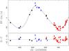 |
Fig. 1 Radial velocity measurements of HIP 8541. The black circles, blue triangles, and red squares represent the UCLES, FEROS, and CHIRON velocities, respectively. The best Keplerian solution is overplotted (black solid line). The post-fit residuals are shown in the lower panel. |
4.2. HIP 74890 b
The velocity variations of HIP 74890 are listed in Table A.2. The RVs were computed from FEROS and UCLES spectra, taken between the beginning of 2009 and mid-2015. A detailed analysis of the RV data revealed a periodic signal, which is superimposed onto a linear trend. The best Keplerian fit is best explained by a giant planet with a projected mass of 2.4 ± 0.3 MJ in a 822-day orbit with a low eccentricity of e = 0.07 ± 0.07. A third object in the system induces a linear acceleration of –33.23 ± 1.46 m s-1 yr-1. The full set of parameters with their uncertainties are listed in Table 2. Using the Winn et al. (2009) relationship, we obtained a mass and orbital distance of the outer object of mcsini> 7.9 MJ and ac> 6.5 AU. Figure 2 shows the HIP 74890 radial velocities.
The Hipparcos and ASAS photometric datasets of this star present a stability of 0.008 mag and 0.013 mag, respectively. No significant peak is observed in the LS periodogram of these two datasets. Similarly, the BVS analysis, CCF variations, and chromospheric activity analysis show neither an indication of periodic variability nor any correlation with the radial velocities.
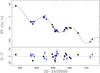 |
Fig. 2 Radial velocity measurements of HIP 74890. The black filled circles and blue triangles correspond to UCLES and FEROS measurements, respectively. The solid line is the best Keplerian solution. The residuals around the fit are shown in the lower panel. |
Orbital parameters.
4.3. HIP 84056 b
The velocity variations of HIP 84056 are listed in Table A.3, and Fig. 3 shows its RV curve. The best orbital solution leads to P = 818.8 ± 12.1 d, mb sini = 2.6 ± 0.3, and e = 0.04 ± 0.04. The full orbital elements solution are listed in Table 2. This planet was independently detected by the PPPS (Wittenmyer et al. 2016). Based on 21 RV epochs, they obtained an orbital period of 885 ± 63 days, a minimum mass of 2.0 ± 0.5 MJ , and an eccentricity of 0.03 ± 0.2, which is in good agreement with our results.
To determine the nature of the periodic RV signal observed in HIP 84056, we performed an activity analysis, as described in Sect. 4.1. We found no significant periodicity or variability of the activity indicators with the observed RVs. Moreover, the photometric analysis of the Hipparcos data reveals a stability of 0.009 mag. Similarly, the rms of the ASAS data is 0.012 mag. These results support the planet hypothesis of the periodic signal detected in the RVs.
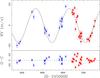 |
Fig. 3 Upper panel: radial velocity measurements of HIP 84056. The blue triangles and red squares correspond to FEROS and CHIRON data, respectively. The best Keplerian solution is overplotted (black solid line). Lower panel: residuals from the Keplerian fit. |
4.4. HIP 95124 b
The RV variations of HIP 95124 are listed in Table A.4 and are plotted in Fig. 4. The orbital parameters are summarized in Table 2. The radial velocities of HIP 95124 are best explained by the presence of a 2.9 ± 0.2 MJ planet with orbital period of P = 562.1 ± 6.0 d and eccentricity e = 0.1 ± 0.07. These derived orbital elements are consistent with the values previously reported by Johnson et al. (2010a)5.
As we did for the other stars described here, we scrutinized the Hipparcos and ASAS photometry to search for any signal with a period similar to that observed in the RV time series, and found a null result. Moreover, the Hipparcos and ASAS rms is 0.007 mag and 0.013 mag. According to Hatzes (2002), this photometric variability is well below the level that mimics the RV amplitude observed in this star. Additionally, the BVS, CCF variations, and S-index variations show no significant correlation with the observed radial velocities.
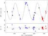 |
Fig. 4 Radial velocities of HIP 95124. The black filled circles, blue triangles, and red squares correspond to UCLES, FEROS, and CHIRON data, respectively. The solid line is the best Keplerian solution. The residuals around the fit are shown in the lower panel. |
5. Preliminary statistical results of the EXPRESS project
After 6 yr of continuous monitoring of a sample comprised of 166 giant stars, we have published a total of 11 substellar companions (including this work), orbiting ten different stars. In addition, using combined data of the EXPRESS and PPPS surveys, we have detected a two-planet system in a 3:5 mean-motion resonance (Wittenmyer et al. 2015) around the giant star HIP 24275. Moreover, Trifonov et al. (2014), recently announced the discovery of a two-planet system around HIP 5364 as part of the Lick Survey (Frink et al. 2002). Since this star is part of our RV program, we have also taken several FECH and CHIRON spectra. The resulting velocities will be presented in a forthcoming paper (Jones et al., in prep.).
In summary, a total of 15 substellar companions to 12 different stars in our sample have been confirmed, plus a number of candidate systems that are currently being followed up (Jones et al., in prep.). These objects have projected masses in the range 1.4–20.0 MJ , and orbital periods between 89 d (0.46 AU) and 2132 d (3.82 AU).
Figure 5 shows the orbital distance versus stellar mass for these 12 systems. The red and blue dashed lines represent radial velocity amplitudes of K = 30 m s-1 (assuming circular orbits), which correspond to ~3σ detection limits6. It can be seen that we can detect planets with MP ≳ 3.0MJ up to a ~ 3 AU (or MP ≳ 2.5MJ at a ~ 2.5 AU) around stars with M⋆ ≲ 2.5 M⊙. For more massive stars, we can only detect those planets orbiting interior to ~2.5 AU. We note that we collected at least 15 RV epochs for each of our targets, with a typical timespan of ~2–3 yr, which allow us to efficiently detect periodic RV signals with K ≳ 30 m s-1 and e ≲ 0.6 via periodogram analysis and visual inspection. Moreover, we obtained additional data for our targets showing RV variability ≳20 m s-1 , including those presenting linear trends. Some of these linear trend systems are brown-dwarf candidates, with orbital periods exceeding the total observational timespan of our survey (P ≳ 2200 d; see Bluhm et al. 2016). We also note that in the case of HIP 67851 c (Jones et al. 2015b), we used ESO archive data to fully cover its orbital period (P = 2132 d; a = 3.82 AU).
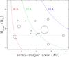 |
Fig. 5 Stellar mass versus semi-major axis of the 12 planetary systems in our sample. The size of the circles is proportional to the planet mass. Multiplanet systems are connected by the dotted lines. The red, green, and blue dashed lines correspond to K = 30 m s-1 , for 1, 2, and 3 MJ planets, respectively. |
5.1. Stellar mass and metallicity
Figure 6 shows a histogram of the planetary occurrence rate as a function of the stellar mass in our sample. The bin width is 0.4 M⊙ and the stellar masses range from 0.9 M⊙ to 3.5 M⊙. The uncertainties were computed according to Cameron (2011), and correspond to 68.3% equal-tailed confidence limits. As can be seen, there is an increase in the detection fraction with the stellar mass between ~1.0 and 2.1 M⊙, reaching a peak in the occurrence rate of  % at M⋆ = 2.1 M⊙. In addition, there is a sharp drop in the occurrence rate at stellar masses ≳2.5 M⊙. In fact, there are 17 stars in our survey in this mass regime, but none of them hosts a planet. We note that, although the observed lack of planets around these stars might be in part explained by the reduced RV sensitivity (see Fig. 5), all of our targets more massive than 2.5 M⊙ present RV variability ≲15 m s-1 . This means that we can also discard planets with MP ≳ 3.0MJ interior to a ~ 3 AU, otherwise we would expect to observe Doppler-induced variability at the ≳20 m s-1 level7. Following the REF15 results, we fitted a Gaussian function to the data, of the form
 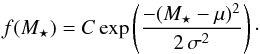 (1)To obtain the values of C, μ and σ, we generated 10000 synthetic datasets, computing the confidence limits for each realization following the Cameron (2011) prescription. After fitting C, μ, and σ for each synthetic dataset, we end up with a probability density distribution for each of these three parameters. We note that we first computed C, and then we fixed it to compute μ and σ, restricting these two parameters to μ ∈ [1.5, 3.0] and σ ∈ [0.0,1.5]. Figure 7 shows our results for the three parameters. The red lines correspond to the smoothed distributions. We obtained the following values:
  ,
,  M⊙, and
  M⊙. The parameters were derived from the maximum value and 68.3% equal-tailed confidence limits of each smoothed distribution.
Although we are dealing with low number statistics, particularly for the upper mass bin, these results are in excellent agreement with previous works. JOHN10, based on a sample of 1266 stars with M⋆ ~ 0.5–2.0 M⊙, showed that the occurrence rate of planets increases linearly with the mass of the host star, reaching a fraction of ~14% at M⋆ ~ 2.0 M⊙. Similarly, based on a sample of 373 giant stars with M⋆ ~ 1.0–5.0 M⊙, REF15 showed that the detection fraction of giant planets present a Gaussian distribution with a peak in the detection fraction of ~8% at ~1.9 M⊙. Additionally, they showed that the occurrence rate around stars more massive than ~2.7 M⊙ is consistent with zero, in good agreement with our findings and also with theoretical predictions. For instance, based on a semi-analytic calculation of an evolving snow-line, Kennedy & Kenyon (2008) showed that the formation efficiency increases linearly from 0.4 to 3.0 M⊙. For stars more massive than 3.0 M⊙, the formation of gas giant planets in the inner region of the protoplanetary disk is strongly reduced. Because of the fast stellar evolution timescale for those massive stars, the snow line moves rapidly to 10–15 AU, preventing the formation of the giant planets in this region.
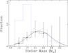 |
Fig. 6 Normalized occurrence rate versus stellar mass for EXPRESS targets with published planets. The dashed blue line corresponds to the parent sample distribution. The solid curve corresponds to the Gaussian fit (Eq. (1)). |
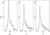 |
Fig. 7 Probability density functions for μ, σ, and C, obtained from a total of 10 000 synthetic datasets. The red lines correspond to the smoothed distributions. |
Figure 8 shows the planet occurrence rate as a function of the stellar metallicity. The symbols and lines are the same as in Fig. 6. The width of the bins is 0.15 dex. It can be seen that the occurrence rate increases with the stellar metallicity, reaching a peak of  % around stars with [Fe/H] = 0.35 dex. This trend seems to be real, despite a relatively high fraction observed in the bin centered at –0.25 dex, which might be explained by the low number statistics for that specific bin. Following the prescription of FIS05, we fitted the metallicity dependence of the occurrence fraction, with a function of the form
 ![\begin{equation} f([{\rm Fe/H}]) = \alpha\,10^{\beta\,[{\rm Fe/H}]}\,. \label{eq2} \end{equation}](/articles/aa/full_html/2016/06/aa28067-16/aa28067-16-eq92.png) (2)Using a similar approach for fitting Eq. (1), we obtained the following values:
(2)Using a similar approach for fitting Eq. (1), we obtained the following values:  and
and  dex-1. Figure 9 shows the probability density distribution of α and β obtained after fitting the synthetic datasets. The functional dependence of the occurrence rate with [Fe/H] (Eq. (2)) is overplotted (solid curve).
This relationship between the occurrence rate and the stellar metallicity is also observed in solar-type stars (Gonzalez 1997; Santos et al. 2001). Moreover, according to REF15, this trend is also present in giant stars. Interestingly, they also showed that there is an overabundance of planets around giant stars with [Fe/H] ~−0.3, similarly to what we found in our sample.
Detection fraction in different stellar mass-metallicity bins.
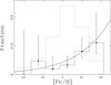 |
Fig. 8 Normalized occurrence rate versus stellar metallicity for EXPRESS targets with published planets. The dashed blue line corresponds to the parent sample distribution. The solid curve is our best fit to Eq. (2). |
To investigate whether one of the two correlations presented above are spurious, we investigated the level of correlation between the stellar mass and metallicity in our sample. Figure 10 shows the mass of the star as a function of the metallicity for all of our targets (filled dots). The open circles are the planet-hosting stars. In the top left corner the mean uncertainty in [Fe/H] and M⋆ is shown. From Fig. 10, it is clear that there is some dependence between these two quantities. The Pearson linear coefficient is r = 0.27, which means that there is a moderate level of correlation. Moreover, if we restrict our analysis to stars with M⋆< 2.5 M⊙, the r-value drops to 0.22 and we obtain a steeper rise in the occurrence rate with the stellar metallicity. Thus, we conclude that the two correlations presented in Figs. 6 and 8 are valid.
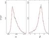 |
Fig. 9 Probability density functions for α and β obtained from a total of 10 000 synthetic datasets. The red lines correspond to the smoothed distributions. |
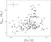 |
Fig. 10 Mass versus metallicity of the 166 giant stars in our survey. The red open circles correspond to the planet-hosting stars. |
In addition, we computed the fraction of our stars hosting planets in the stellar mass-metallicity space using the same bins size presented in REF15. These results are listed in Table 3. Columns 1 and 2 correspond to the stellar metallicity and mass bins, each of 0.16 dex and 0.8 M⊙, respectively. The number of stars with detected planets (np), number of stars in the bin (ns), and the fraction of stars with planets in each bin (f) are listed in Cols. 3–5. It can be seen that the highest fraction is obtained in the bin centered at 1.4 M⊙ and 0.12 dex (f = 9.4 ), which is slightly higher than the value of the bin with the same metallicity, but centered at 2.2 M⊙ (
 ). Interestingly, REF15 found a similar trend, i.e., they also obtained the highest fraction in these two mass-metallicity bins, although they claim higher values for f. We also analyzed the combined results of the two surveys. These are listed in Cols. 6–8 in Table 3. It can be seen that the overall trend is unaffected, but the uncertainties in the planet fraction are smaller.
Finally, to understand whether the combined results are affected by systematic differences in the stellar parameters derived independently by the two surveys, we compared the resulting metallicities of the Lick Survey (listed in REF15) with those derived using our method. We used a total of 16 stars, of which 12 are common targets. We measured a difference of Δ([Fe/H])= 0.03 dex ± 0.11 dex, showing the good agreement between the two methods8. Similarly, we compared the masses of the stars derived by the two surveys. We found that our stellar masses are on average larger by Δ(M⋆) = 0.15 ± 0.37 M⊙, which corresponds to a ratio of 1.07 ± 0.18. For comparison, Niedzielski et al. (2016) also found that our stellar masses are overestimated with respect to their values by a factor of 1.15 ± 0.10. We also note that the planet-hosting star HIP 5364 is a common target of the two surveys. They obtained Teff = 4528 ± 19 K and [Fe/H] = 0.07 ± 0.1 dex. Using these values they derived a mass of 1.7 ± 0.1 M⊙ for this star (Trifonov et al. 2014), significantly lower than our value of 2.4 ± 0.3 M⊙. This shows that the combined results of the Lick and EXPRESS surveys should be taken with caution. Certainly, a more detailed comparison between the stellar parameters, as well as their completeness, derived independently by the two surveys will allow us to check the validity of these combined results.
5.2. Multiple-planet systems
Of the 12 planet-hosting stars in our sample, HIP 5364, HIP 24275, and HIP 67851 host planetary systems with at least two giant planets. This means that 25% of the parent stars host a multiple system. Considering the full sample, this yields a ~2% fraction of multiple systems, i.e., sytems that are comprised of two or more giant planets (Mp> 1.0 MJ ). This number is a lower limit, since there are several other systems in our sample whose velocities are compatible with the presence of a distant giant planet, but still need confirmation (e.g., HIP 74890, presented in Sect. 4.2).
If we consider all of the known planet-hosting giant stars (log g ≲ 3.6), around 10% of them host a planetary system including at least two giant planets. This fraction is significantly higher than solar-type stars. There are only 21 such systems among dwarf stars9, although most of the RV surveys have targeted this type of stars. Moreover, planets are easier to detect via precision RVs around solar-type stars because they are, on average, less massive and have p-mode oscillations that are much weaker than for giant stars (Kjeldsen & Bedding 1995), which translates into larger amplitudes with a lower level of RV noise. This observational result is a natural extension of the known mass distribution of single-planet systems orbiting evolved stars, which is characterized by an overabundance of super-Jupiter-like planets (e.g., Lovis & Mayor 2007; Döllinger et al. 2009; Jones et al. 2014). This result also reinforces the observed positive correlation between the stellar and planetary mass, in the sense that more massive stars tend to form not only more massive single planets, but also more massive multiplanet systems.
6. Summary and discussion
In this work we present precision radial velocities of four giant stars that have been targeted by the EXPRESS project over the past six years. These velocities show periodic signals with semi-amplitudes between ~50–100 m s-1 , which are likely caused by the Doppler shift induced by orbiting companions. We performed standard tests (chromospheric emission, line bisector analysis, and photometric variability) aimed at studying whether these RV signals have an intrinsic stellar origin. We found no correlation between the stellar intrinsic indicator with the observed velocities. Therefore, we conclude that the most probable explanation of the periodic RV signals observed in these stars is the presence of substellar companions. The best Keplerian fit to the RV data of the four stars leads to minimum masses between mb sini = 2.4–5.5 MJ and orbital periods P = 562–1560 days. Interestingly, all of them have low eccentricities (e ≤ 0.16), confirming that most of the giant planets orbiting evolved stars present orbital eccentricities ≲0.2 (Schlaufman & Winn 2013; Jones et al. 2014). The RVs of HIP 74890 also reveal the presence of a third object at large orbital separation (a> 6.5 AU). The RV trend induced by this object is most likely explained by a brown dwarf or a stellar companion.
We also present a statistical analysis of the mass-metallicity correlations of the planet-hosting stars in our sample. Drawn from a parent sample of 166 stars, this subsample of 12 stars hosts a total of 15 giant planets. We show that the fraction of giant planets f increases with the stellar mass in the range between ~1.0 and 2.1 M⊙, even though planets are more easily detected around less massive stars. For comparison, we obtained  % for M⋆ ~ 1.3 M⊙, and a peak of % for stars with M⋆ ~ 2.1 M⊙. These results are in good agreement with previous works showing that the occurrence rate of giant planets exhibits a positive correlation with the stellar mass up to M⋆ ~ 2.0 M⊙ (e.g., JOHN10; REF15). For stars more massive than ~2.5 M⊙, the fraction of planets is consistent with zero. We fitted the overall occurrence distribution with a Gaussian function (see Eq. (1)), obtaining the following parameters: , M⊙, and σ = 0.64
 M⊙.
M⊙.
Similarly, we studied the occurrence rate of giant planets as a function of the stellar metallicity. We found an overabundance of planets around metal-rich stars, with a peak of  % for stars with [Fe/H] ~ 0.35 dex. We fitted the metallicity dependence of the occurrence rate with a function of the form f = α10β [Fe/H], obtaining the following parameter values: α = 0.061
 and β = 1.27
 dex-1. Our power-law index β lies between the values measured by JOHN10 (β = 1.2 ± 0.2) and FIS05 (β = 2.0). Thus, our results suggest that the PMC observed in solar-type stars is also present in intermediate-mass (M⋆ ≳ 1.5 M⊙) evolved stars, in agreement with REF15 results.
Finally, we investigated the fraction of multiple planetary systems comprised of two or more giant planets. Out of the 12 systems presented above, 3 of them contain two giant planets, which is a significant fraction of the total number of these planetary systems. If we also consider multiplanet systems published by other RV surveys, we find that there is a significantly higher fraction around intermediate-mass evolved stars than around solar-type stars. This result is not surprising since different works have shown that giant planets are more frequent around intermediate-mass stars (Döllinger et al. 2009; Bowler et al. 2010), which is also supported by theoretical predictions (Kennedy & Kenyon 2008). In addition, planets tend to be more massive around intermediate-mass stars than around solar-type stars (e.g., Lovis & Mayor 2007; Döllinger et al. 2009; Jones et al. 2014). Thus, we conclude that the high fraction of multiple systems observed in giant stars is a natural consequence of the planet formation mechanism around intermediate-mass stars.
Source: http://www.exoplanets.org/
One of these planets (HD 122430 b) was shown not to be a real planet (Soto et al. 2015).
For FEROS and CHIRON data, the RV noise is dominated by stellar pulsations, that induce velocity variability of ~5–10 m s-1 level in our targets. In fact, according to Kjeldsen & Bedding (1995), only 4 of our targets are expected to present velocity variations larger than 10 m s-1 . In the case of FECH data, the instrumental uncertainty is comparable to the stellar pulsations noise.
Source: http://exoplanets.org
Acknowledgments
M.J. acknowledges financial support from Fondecyt project #3140607 and FONDEF project CA13I10203. A.J. acknowledges support from Fondecyt project #1130857, the Ministry of Economy, Development, and Tourism’s Millennium Science Initiative through grant IC120009, awarded to The Millennium Institute of Astrophysics (MAS). P.R. acknowledges funding by the Fondecyt project #1120299. F.O. acknowledges financial support from Fondecyt project #3140326 and from the MAS. J.J., P.R., and A.J. acknowledge support from CATA-Basal PFB-06. H.D. acknowledges financial support from FONDECYT project #3150314. This research has made use of the SIMBAD database and the VizieR catalogue access tool, operated at CDS, Strasbourg, France.
References
- Alibert, Y., Mordasini, C., & Benz, W. 2004, A&A, 417, 25 [Google Scholar]
- Baranne, A., Queloz, D., Mayor, M., et al. 1996, A&A, 119, 373 [Google Scholar]
- Bluhm, P., Jones, M. I., Vanzi, L., et al. 2016, A&A, submitted [Google Scholar]
- Boisse, I., Bouchy, F., Hebrard, G., et al. 2011, A&A, 528, A4 [NASA ADS] [CrossRef] [EDP Sciences] [Google Scholar]
- Borucki, W. J., Koch, D., Basri, G., et al. 2010, Science, 327, 977 [NASA ADS] [CrossRef] [PubMed] [Google Scholar]
- Bowler, B. P., Johnson, J. A., Marcy, G. W., et al. 2010, ApJ, 709, 396 [NASA ADS] [CrossRef] [Google Scholar]
- Butler, R. P., Marcy, G. W., Williams, E., et al. 1996, PASP, 108, 500 [NASA ADS] [CrossRef] [Google Scholar]
- Cameron, E. 2011, PASA, 28, 128 [NASA ADS] [CrossRef] [Google Scholar]
- Diego, F., Charalambous, A., Fish, A. C., & Walker, D. D. 1990, Proc. Soc. Photo-Opt. Instr. Eng., 1235, 562 [Google Scholar]
- Döllinger, M. P., Hatzes, A. P., Pasquini, L., Guenther, E. W., & Hartmann, M. 2009, A&A, 505, 1311 [NASA ADS] [CrossRef] [EDP Sciences] [Google Scholar]
- Figueira, P., Marmier, M., Bonfils, X., et al. 2010, A&A, 513, A8 [NASA ADS] [CrossRef] [EDP Sciences] [Google Scholar]
- Fischer, D. A., & Valenti, J. 2005, ApJ, 622, 1102 [NASA ADS] [CrossRef] [Google Scholar]
- Frink, S., Mitchell, D. S., Quirrenbach, A., et al. 2002, ApJ, 576, 478 [NASA ADS] [CrossRef] [MathSciNet] [Google Scholar]
- Gonzalez, G. 1997, MNRAS, 285, 403 [NASA ADS] [CrossRef] [Google Scholar]
- Hatzes, A. P. 2002, AN, 323, 392 [Google Scholar]
- Hekker, S., & Meléndez, J. 2007, A&A, 475, 1003 [NASA ADS] [CrossRef] [EDP Sciences] [Google Scholar]
- Hekker, S., Snellen, I. A. G., Aerts, C., et al. 2008, A&A, 480, 215 [NASA ADS] [CrossRef] [EDP Sciences] [Google Scholar]
- Huélamo, N., Figueira, P., Bonfils, X., et al. 2008, A&A, 489, 9 [Google Scholar]
- Ida, S., & Lin, D. N. C. 2004, ApJ, 604, 388 [NASA ADS] [CrossRef] [PubMed] [Google Scholar]
- Jenkins, J. S., Jones, H. R. A., Pavlenko, Y., et al. 2008, A&A, 485, 571 [NASA ADS] [CrossRef] [EDP Sciences] [Google Scholar]
- Jenkins, J. S., Murgas, F., Rojo, P., et al. 2011, A&A, 531, A8 [NASA ADS] [CrossRef] [EDP Sciences] [Google Scholar]
- Jofre, E., Petrucci, R., Saffe, C., et al. 2015, A&A, 574, A50 [NASA ADS] [CrossRef] [EDP Sciences] [Google Scholar]
- Johnson, J. A., Butler, R. P., Marcy, G. W., et al. 2007, ApJ, 670, 833 [NASA ADS] [CrossRef] [Google Scholar]
- Johnson, J. A., Howard, A. W., Bowler, B. P., et al. 2010a, PASP, 122, 701 [NASA ADS] [CrossRef] [Google Scholar]
- Johnson, J. A., Aller, K. M., Howard, A. W., & Crepp, J. R. 2010b, PASP, 122, 905 [NASA ADS] [CrossRef] [Google Scholar]
- Jones, M. I., Jenkins, J. S., Rojo, P., & Melo, C. H. F. 2011, A&A, 536, A71 [NASA ADS] [CrossRef] [EDP Sciences] [Google Scholar]
- Jones, M. I., Jenkins, J. S., Rojo, P., Melo, C. H. F., & Bluhm, P. 2013, A&A, 556, A78 [NASA ADS] [CrossRef] [EDP Sciences] [Google Scholar]
- Jones, M. I., Jenkins, J. S., Bluhm, P., Rojo, P., & Melo, C. H. F. 2014, A&A, 566, A113 [NASA ADS] [CrossRef] [EDP Sciences] [Google Scholar]
- Jones, M. I., Jenkins, J. S., Rojo, P., Melo, C. H. F., & Bluhm, P. 2015a, A&A, 573, A3 [NASA ADS] [CrossRef] [EDP Sciences] [Google Scholar]
- Jones, M. I., Jenkins, J. S., Rojo, P., Olivares, F., & Melo, C. H. F. 2015b, A&A, 580, A14 [NASA ADS] [CrossRef] [EDP Sciences] [Google Scholar]
- Kaufer, A., Stahl, O., Tubbesing, S., et al. 1999, The Messenger, 95, 8 [Google Scholar]
- Kennedy, G. M., & Kenyon, S. J. 2008, ApJ, 673, 502 [NASA ADS] [CrossRef] [Google Scholar]
- Kjeldsen, H., & Bedding, T. R. 1995, A&A, 293, 87 [NASA ADS] [Google Scholar]
- Lovis, C., & Mayor, M. 2007, A&A, 472, 657 [NASA ADS] [CrossRef] [EDP Sciences] [Google Scholar]
- Maldonado, J., Villaver, E., & Eiroa, C. 2013, A&A, 554, A84 [NASA ADS] [CrossRef] [EDP Sciences] [Google Scholar]
- Mayor, M., & Queloz, D. 1995, Nature, 378, 355 [NASA ADS] [CrossRef] [Google Scholar]
- Meschiari, S., Wolf, A. S., Rivera, E., et al. 2009, PASJ, 121, 1016 [Google Scholar]
- Murray, N., & Chaboyer, B. 2002, ApJ, 566, 442 [NASA ADS] [CrossRef] [Google Scholar]
- Niedzielski, A., Deka-Szymankiewicz, B., Adamczyk, M., et al. 2016, A&A, 585, A73 [NASA ADS] [CrossRef] [EDP Sciences] [Google Scholar]
- Pasquini, L., Döllinger, M. P., Weiss, A., et al. 2007, A&A, 473, 979 [NASA ADS] [CrossRef] [EDP Sciences] [Google Scholar]
- Pojmanski, G. 1997, Acta Astron., 47, 467 [NASA ADS] [Google Scholar]
- Pollack, J. B., Hubickyj, O., Bodenheimer, P., et al. 1996, Icarus, 124, 62 [NASA ADS] [CrossRef] [Google Scholar]
- Queloz, D., Henry, G. W., Sivan, J. P., et al. 2001, A&A, 379, 279 [NASA ADS] [CrossRef] [EDP Sciences] [Google Scholar]
- Reffert, S., Bergmann, C., Quirrenbach, A., et al. 2015, A&A, 574, A116 [NASA ADS] [CrossRef] [EDP Sciences] [Google Scholar]
- Salasnich, B., Girardi, L., Weiss, A., & Chiosi, C. 2000, A&A, 361, 1023 [NASA ADS] [Google Scholar]
- Santos, N. C., Israelian, G., & Mayor, M. 2001, A&A, 373, 1019 [NASA ADS] [CrossRef] [EDP Sciences] [Google Scholar]
- Sato, B., Eiji, K., Yoichi, T., et al. 2005, PASJ, 57, 97 [NASA ADS] [CrossRef] [Google Scholar]
- Scargle, J. D. 1982, ApJ, 263, 835 [NASA ADS] [CrossRef] [Google Scholar]
- Schlaufman, K., & Winn, J. 2013, ApJ, 772, 143 [NASA ADS] [CrossRef] [Google Scholar]
- Sneden, C. 1973, ApJ, 184, 839 [NASA ADS] [CrossRef] [Google Scholar]
- Soto, M., Jenkins, J. S., & Jones, M. I. 2015, MNRAS, 451, 3131 [NASA ADS] [CrossRef] [Google Scholar]
- Tinney, C. G., Wittenmyer, R. A., Butler, R. P., et al. 2001, ApJ, 732, 31 [NASA ADS] [CrossRef] [Google Scholar]
- Tokovinin, A., Fischer, D. A., Bonati, M., et al. 2013, PASP, 125, 1336 [NASA ADS] [CrossRef] [Google Scholar]
- Toner, C. G., & Gray, D. F. 1988, ApJ, 334, 1008 [NASA ADS] [CrossRef] [Google Scholar]
- Trifonov, T., Reffert, S., Tan, X., Lee, M. H., & Quirrenbach, A. 2014, A&A, 568, A64 [NASA ADS] [CrossRef] [EDP Sciences] [Google Scholar]
- Van Leeuwen, F. 2007, A&A, 474, 653 [NASA ADS] [CrossRef] [EDP Sciences] [Google Scholar]
- Winn, J. N., Johnson, J. A., Albrecht, S., et al. 2009, ApJ, 703, 99 [Google Scholar]
- Wittenmyer, R. A., Endl, M., Wang, L., et al. 2011, ApJ, 743, 184 [NASA ADS] [CrossRef] [Google Scholar]
- Wittenmyer, R. A., Horner, J., Tuomi, M., et al. 2012, ApJ, 753, 169 [NASA ADS] [CrossRef] [Google Scholar]
- Wittenmyer, R. A., Johnson, J. A., Butler, R. P., et al. 2015, MNRAS, accepted [Google Scholar]
- Wittenmyer, R. A, Butler, R. P., Wang, L., et al. 2016, MNRAS, 455, 1398 [NASA ADS] [CrossRef] [Google Scholar]
Appendix A: Radial velocity tables
Radial velocity variations of HIP 8541.
Radial velocity variations of HIP 74890.
Radial velocity variations of HIP 84056.
Radial velocity variations of HIP 95124.
All Tables
All Figures
|
Fig. 1 Radial velocity measurements of HIP 8541. The black circles, blue triangles, and red squares represent the UCLES, FEROS, and CHIRON velocities, respectively. The best Keplerian solution is overplotted (black solid line). The post-fit residuals are shown in the lower panel. |
| In the text | |
|
Fig. 2 Radial velocity measurements of HIP 74890. The black filled circles and blue triangles correspond to UCLES and FEROS measurements, respectively. The solid line is the best Keplerian solution. The residuals around the fit are shown in the lower panel. |
| In the text | |
|
Fig. 3 Upper panel: radial velocity measurements of HIP 84056. The blue triangles and red squares correspond to FEROS and CHIRON data, respectively. The best Keplerian solution is overplotted (black solid line). Lower panel: residuals from the Keplerian fit. |
| In the text | |
|
Fig. 4 Radial velocities of HIP 95124. The black filled circles, blue triangles, and red squares correspond to UCLES, FEROS, and CHIRON data, respectively. The solid line is the best Keplerian solution. The residuals around the fit are shown in the lower panel. |
| In the text | |
|
Fig. 5 Stellar mass versus semi-major axis of the 12 planetary systems in our sample. The size of the circles is proportional to the planet mass. Multiplanet systems are connected by the dotted lines. The red, green, and blue dashed lines correspond to K = 30 m s-1 , for 1, 2, and 3 MJ planets, respectively. |
| In the text | |
|
Fig. 6 Normalized occurrence rate versus stellar mass for EXPRESS targets with published planets. The dashed blue line corresponds to the parent sample distribution. The solid curve corresponds to the Gaussian fit (Eq. (1)). |
| In the text | |
|
Fig. 7 Probability density functions for μ, σ, and C, obtained from a total of 10 000 synthetic datasets. The red lines correspond to the smoothed distributions. |
| In the text | |
|
Fig. 8 Normalized occurrence rate versus stellar metallicity for EXPRESS targets with published planets. The dashed blue line corresponds to the parent sample distribution. The solid curve is our best fit to Eq. (2). |
| In the text | |
|
Fig. 9 Probability density functions for α and β obtained from a total of 10 000 synthetic datasets. The red lines correspond to the smoothed distributions. |
| In the text | |
|
Fig. 10 Mass versus metallicity of the 166 giant stars in our survey. The red open circles correspond to the planet-hosting stars. |
| In the text | |
Current usage metrics show cumulative count of Article Views (full-text article views including HTML views, PDF and ePub downloads, according to the available data) and Abstracts Views on Vision4Press platform.
Data correspond to usage on the plateform after 2015. The current usage metrics is available 48-96 hours after online publication and is updated daily on week days.
Initial download of the metrics may take a while.