| Issue |
A&A
Volume 589, May 2016
|
|
|---|---|---|
| Article Number | A131 | |
| Number of page(s) | 7 | |
| Section | Astrophysical processes | |
| DOI | https://doi.org/10.1051/0004-6361/201628097 | |
| Published online | 25 April 2016 | |
Alfvén-dynamo balance and magnetic excess in magnetohydrodynamic turbulence
1 LPP, École Polytechnique, Route de Saclay, 91120 Palaiseau, France
e-mail: This email address is being protected from spambots. You need JavaScript enabled to view it.
2 Technische Universität Berlin, Zentrum für Astronomie und Astrophysik, Hardenbergstr. 36A, 10623 Berlin, Germany
3 Università di Firenze, Dipartimento di Fisica e Astronomia Largo Fermi, 50125 Firenze, Italy and Royal Observatory of Belgium, SIDC/STCE, 3 avenue circulaire, 1180 Brussels, Belgium
Received: 8 January 2016
Accepted: 9 March 2016
Abstract
Context. Three-dimensional magnetohydrodynamic (3D MHD) turbulent flows with initially magnetic and kinetic energies at equipartition spontaneously develop a magnetic excess (or residual energy) in both numerical simulations and the solar wind. Closure equations obtained in 1983 describe the residual spectrum as resulting from a balance between a dynamo source proportional to the total energy spectrum and a linear Alfvén damping term. A good agreement was found in 2005 with incompressible simulations; however, recent solar wind measurements disagree with these results.
Aims. The previous dynamo-Alfvén theory is generalized to a family of models, leading to simple relations between residual and total energy spectra. We want to assess these models in detail against MHD simulations and solar wind data.
Methods. We tested the family of models against compressible decaying MHD simulations with a low Mach number, low cross-helicity, and zero-mean magnetic field with or without expansion terms (EBM; expanding box model).
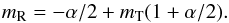
Results. A single dynamo-Alfvén model is found to describe correctly both solar wind scalings and compressible simulations without or with expansion. This model is equivalent to the 1983–2005 closure equation, but it incorporates the critical balance of nonlinear turnover and linear Alfvén times, while the dynamo source term remains unchanged. We elucidate the discrepancy with previous incompressible simulations. The model predicts a linear relation between the spectral slopes of total and residual energies mR = −1/2 + 3/2mT. By examining previous solar wind data, our relation is found to be valid for any cross-helicity, and is even better at high cross-helicity with the total energy slope varying from 1.7 to 1.55.
Key words: magnetohydrodynamics (MHD) / plasmas / turbulence / solar wind
© ESO, 2016
1. Introduction
Three-dimensional magnetohydrodynamic (3D MHD) turbulent flows with initial equipartition of magnetic ( ) and kinetic (
 ) spectral energy density spontaneously develop a magnetic excess. In the solar wind, the magnetic excess in the k− 5/3 scaling range is largest in the cold, slow wind with no or small mean field (e.g., Grappin et al. 1991; Bruno et al. 2007). Recent measurements have revealed that when the relative cross-helicity
  is smaller than 0.6, the residual energy
  adopts the scaling k-2 (Chen et al. 2013), while the total energy
  scales as k− 5/3.
The origin of the magnetic excess in the solar wind has been attributed to different physical mechanisms: (i) remnants of quasi-stationary solar magnetic structures (Bruno et al. 2007); (ii) formation and persistence of current sheets (Matthaeus & Lamkin 1986); (iii) selective decay of ideal invariants (Stribling & Matthaeus 1991); and (iv) fully developed turbulence. In the latter case, which interests us here, the residual energy spectrum results from the competition between the linear damping of Alfvén waves by the local mean field, the Alfvén effect (Kraichnan 1965), and the magnetic stretching, which is the source proportional to the total energy spectrum (Grappin et al. 1983; Müller & Grappin 2005, MG05). We call it the Alfvén-dynamo scenario. The model, in its stationary version, allows us to predict the residual energy spectrum, given the total energy spectrum. In particular, it predicts that the slopes of total energy (mT) and residual energy (mR) satisfy  (1)which yields mR = 2 only if mT = 3/2; this is at variance with the solar wind case, which shows on average mR ≃ 2 and mT ≃ 5/3. The model discussed here is not a cascade theory: the magnetic excess is not a inviscid invariant, it is assumed to be the passive by-product of the two effects mention above. Hence, the validity of our model is potentially more general than the validity of, for example, the Kolmogorov regime (e.g., Lee et al. 2010).
The isotropic closure approximation (eddy-damped-quasi-normal or edqnm) used to derive the dynamo-Alfvén equation has been criticized. Indeed, the small-scale dynamics in MHD turbulence should be dominated by motions perpendicular to the large-scale magnetic field; this, in turn, should strongly reduce the influence of the Alfvén effect, which is a basic part of the theory (Biskamp 2003, end of Chap. 6). Several attempts have been made since then to include anisotropy into the edqnm closure (Gogoberidze et al. 2012; Boldyrev et al. 2012); however in the case of a strong cascade with no global mean field, these attempts lead to the prediction  , at variance with our numerical findings and also the solar wind as shown in this work.
Our aim here is (i) to investigate whether one can recover the solar wind regime via numerical simulations of either standard compressible 3D MHD equations or 3D expanding box model (EBM) equations, that is, compressible MHD including expansion terms (Grappin et al. 1993; Grappin & Velli 1996); (ii) find an appropriate framework for a Alfvén-dynamo scenario describing simulations and the solar wind that takes anisotropy into account.
We consider the case with zero mean field and low cross-helicity, and small Mach number. Although the solar wind is rarely, strictly in a zero mean field configuration (brms/B0 ≃ 0.5 for a period range from 10 to 2 h, where B0 is the mean magnetic field at the 10 h scale, e.g., Roberts 1989), the magnetic excess is dominant close to the heliospheric current sheet where the mean field is small, which is the configuration studied by Chen et al. (2013).
To provide a diagnostic tool for our simulations, we first generalize formally the Alfvén dynamo balance derived from edqnm, by considering different simple expressions for the characteristic times of the dynamo source and the Alfvén sink. These return different scaling predictions for the residual energy spectrum, given the spectral slope for total energy, quantitative predictions for the relative levels of both spectra, and also relaxation curves. We test these different models against our simulations.
We find that compressible MHD simulations, both standard and with expansion (EBM), show a quasi-stationary regime corresponding to that found in the solar wind. This quasi-stationary state is well described, qualitatively (scaling) and quantitatively (amplitude) if we keep the dynamo source term as in the 1983 edqnm scenario, but change the Alfvén sink, taking the critical balance between nonlinear coupling and linear propagation into account. The relation between the residual and total energy spectral slopes predicted by our theory applies not only to the zero cross-helicity wind, but also to high-speed streams with relative cross-helicity close to unity and shallower spectral slopes.
We show that incompressible MG05 simulations differ from the compressible simulations studied here insofar as the scaling law for the residual energy actually depends on the kind of spectrum used, whether reduced or isotropized. Such a dependence is not observed in the compressible simulations considered here.
The plan is as follows. First we derive the family of Alfvén-dynamo models relating the residual and total energy spectra. Then we examine direct simulations of compressible MHD with low Mach number, both with and without expansion terms in the light of the different Alfvén-dynamo models. The last section is a discussion.
2. Generalizing the Alfvén-dynamo model
The Alfvén dynamo model is obtained starting from the incompressible MHD equations and using the edqnm spectral closure. It leads to a closed system of equations relating the different second-order moments of the system. The general form (with Ek denoting either the kinetic, magnetic, or residual energy spectrum) is ∂tEk = ∫dpdqkθEpEq. In the case of the residual energy, the integral may be separated into nonlocal and local contributions, leading to a linear damping term and a nonlinear source, respectively. This can be written as 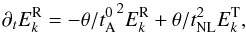 (2)where the characteristic times
  and tNL are (the magnetic field is expressed in units of Alfvén velocity)
  and θ is the relaxation time of triple correlations (in principle
  , see below). The form of the source term is local, while some authors (e.g., Alexakis et al. 2005) claim that kinetic-magnetic exchange (other than the simple Alfvén effect) should show important nonlocal contributions. However, (i) Aluie & Eyink (2010) criticized the methodology of this work; (ii) a workable nonlocal model would be very difficult to build, and as we show here, a local formulation works well in predicting the relation between total and residual energies.
We generalize the edqnm model by writing, instead of Eq. (2), 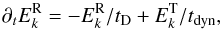 (5)where the two timescales, tD (damping time) and tdyn (dynamo time) can be chosen independently one from another. This leads to the equilibrium solution
 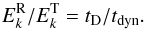 (6)The edqnm model is described by Eq. (2) with
  , and is thus equivalent to Eq. (5) with
  and
and  , which leads to
  .
.
Other expressions of the damping and dynamo times lead to the general family of residual-total energy relations, 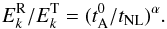 (7)This leads to explicit relations between residual and total energy spectra after replacing the nonlinear time as a function of the total energy spectrum, as in Eq. (4),
  (8)Also, the following relation holds between spectral slopes (
 ):
):  (9)Different values of α can be obtained by using the following expressions of the damping and dynamo timescales in terms of the basic timescales and tNL:
 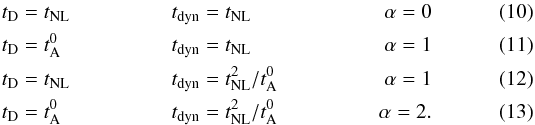 As a rule (except perhaps at the largest scales), one has
  with the inequality becoming stronger at small scales. The first scenario (α = 0, damping and dynamo both based on the nonlinear time tNL) is the simplest of all (Gogoberidze et al. 2012): it leads to an extreme regime with at all scales. This regime is far from both the solar wind and numerical results.
The last scenario with fast damping and slow dynamo based on the long diffusive time , is the edqnm prediction studied in MG05; it leads to α = 2, hence to a fast decreasing residual spectrum with slope mR = 7/3 when mT = 5/3.
The intermediate scenarios (fast damping and dynamo, and slow damping and dynamo, respectively) both lead to α = 1, and hence to mR = 2 when mT = 5/3: they are thus candidates for the description of solar wind dynamics.
3. Numerical results
In this section we consider two decaying compressible simulations with zero mean field, low cross-helicity and resolution 5123: (i) 3D MHD (run A); (ii) 3D EBM (run B). In both cases, the initial Mach number is small (and remains so), thus minimizing compressible effects. Our main issue in this section is to assess Eq. (7): are the numerical results for equilibrium residual energy well described by one of the two algebraic models α = 1 or α = 2, and, accordingly, do the spectral scalings satisfy the corresponding Eq. (9)?
3.1. Compressible turbulence
The first run (A) has random isotropic initial conditions with urms = brms = 1, ∇.u = 0, equal magnetic and kinetic energies with spectra confined to k ≤ 2. Initial relative cross-helicity is 0.17, density is unity, pressure is uniform with sound speed cs = (5/3 P/ρ)1/2 ≃ 8, initial Mach number M0 = urms/cs ≃ 0.12. The domain is a cube of size L0 = 2π.
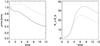 |
Fig. 1 Run A (compressible MHD). a) Kinetic (solid line) and magnetic (dotted) rms amplitudes; b) kinetic (solid line) and magnetic (dotted) Taylor wavenumbers vs. time. |
The evolution of rms velocity (solid line) and magnetic (dotted line) fluctuations versus time is shown in the left panel of Fig. 1, during 12 nonlinear times 1/(k0urms(t = 0)). The Taylor wavenumbers computed on the kinetic (solid) and magnetic (dotted) energy spectrum are shown in the right panel. One sees that the kinetic energy is transferred to magnetic energy in about two nonlinear times, while small scales wait up to about six nonlinear times to be fully excited, as indicated by the peaks of the Taylor wavenumbers. The relative cross-helicity (not shown in the figure) increases during the run from 0.17 to about 0.3.
We consider now reduced one-dimensional (1D) energy spectra E(kx), which are defined from the 3D spectral energy density E3 as 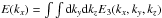 and the same for reduced spectra versus ky or kz. For run A with no expansion and no mean field, all directions should be equivalent; we thus use for all quantities the average of the three reduced spectra, i.e.,
  (14)
(14)
To reveal the spectral slopes of the different reduced spectra, we show in Fig. 2a the total, residual, magnetic, and kinetic energies averaged during the time interval 10 ≤ t ≤ 12 compensated by the slopes k− 5/3, k-2, k− 5/3, k− 3/2, respectively. The averages are made on 209 outputs, after expressing (by interpolating on a fixed grid) the spectra versus the ratio k/kd, where kd is the wavenumber associated with a peak of the instantaneous spectrum of the current, namely of k2EM(k). Plateaus are seen to develop in the range 0.1 ≤ k/kd ≤ 1, thus showing good agreement with spectral slopes measured in the solar wind. The same set of slopes has been found recently in the two-dimensional (2D) hybrid simulations by Franci et al. (2015).
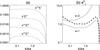 |
Fig. 2 Run A. Energy spectra averaged during time interval 10 ≤ t ≤ 12. Wavenumbers are normalized by the dissipative wavenumber kd for which k2EM(k) is maximum; see text. a) From top to bottom: total, residual, magnetic, and kinetic energies, compensated resp. by k− 5/3, k-2, k− 5/3, k− 3/2. Spectra are arbitrarily shifted vertically. b) Normalized residual energy |

Figure 2b allows us to assess the Alfvén-dynamo scenario by showing the residual spectra normalized by the α-model prediction with successively α = 1 and α = 2. More precisely, one shows  (15)where
 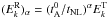 is the equilibrium solution Eq. (7).
The solid curve shows the normalization by the α = 1 prediction and the dotted curve indicates the normalization by the α = 2 prediction. All spectra versus k/kd are again averaged over the 209 spectra stored during the time interval 10 ≤ t ≤ 12. One sees that in the inertial range 0.1 ≤ k/kd ≤ 1, only the α = 1 normalization shows a plateau, indicating that the α = 1 scenario catches the basic physics, in agreement with the slopes (mT,mR) = (5/3,2) obtained for the total and residual spectra in Fig. 2a.
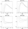 |
Fig. 3 Run A. Time variation of spectral energy density at specific wavenumbers k = 4,8,16,32, resp. solid, dotted, dashed, dot-dashed lines. a) Total energy times k5/3b) residual energy times k2; c) residual energy |


A still better quantitative agreement can be obtained if we use for the stretching time the advection time: tNL = 1/(ku) instead of Eq. (4) (which allowed us to close the problem). This gives a measured/predicted ratio closer to unity in the inertial range, as shown by the dashed curve in Fig. 2b.
To give an idea of how the spectra evolve with time, we show in Fig. 3 the evolution of spectral energy density at five wavenumbers: k = 4,8,16,32, for the four quantities: (a) total; (b) residual; (c) residual energy normalized by α = 1 model; and (d) residual energy normalized by α = 2 model. The total energy is multiplied by k5/3 and the residual energy by k2. Total energies at k = 8,16,32 are seen to collapse at about t ≥ 7, revealing the formation of the k− 5/3 inertial range. At about the same time, the collapse of residual energy curves reveal the formation of the k-2 range. The modes 4 to 32, which are normalized by the α = 1 model, also show in panel c a nice collapse toward a value close to unity. In contrast, modes normalized by the α = 2 model remain significantly scattered.
3.2. Turbulence with expansion
We now consider with run B the 3D MHD equations modified by the expansion (EBM; Grappin et al. 1993). The EBM equations allow us to follow the evolution of a plasma volume embedded in a uniform, given radial flow with speed U0 as in the solar wind. The radial flow cannot be eliminated by a plain Galilean transformation and forces the plasma volume to expand in directions perpendicular to the radial. This leads to many genuine effects specific to solar wind turbulence: (i) quadratic invariants are lost and replaced by first order invariants (as mass, momentum, angular momentum, and magnetic flux); (ii) cascade isotropy is lost, as the turbulent cascade is stronger in the radial direction (Dong et al. 2014). The expansion itself already provides a large-scale source of magnetic excess, as it selectively decreases only one component (the radial one) of the magnetic field in Alfvén speed units and two components of the velocity field (e.g., Zhou & Matthaeus 1990; Oughton & Matthaeus 1995; Grappin et al. 1993; Dong et al. 2014).
We consider initially an isotropic 1 /k large-scale spectrum to mimic the large-scale fossil 1 /f spectrum observed in the wind (Bruno & Carbone 2013). The Mach number is ≃0.1 as for run A; kinetic velocity and magnetic fluctuations are at equipartition, and ∇.u = 0. The wind expansion rate normalized to the large-scale nonlinear time is initially  , where L0 is the initial size of the domain (with aspect ratio unity), and R0 the initial distance. This means that initially most of the spectral range (that with k ≥ 2) has a nonlinear time shorter than the local transit time te = R0/U0. This leaves room for an inertial range to develop, together with specific spectral anisotropy that is characteristic of turbulence with expansion (see Dong et al. 2014; Verdini & Grappin 2015). Evolution is followed from time t = 0 up to t = 3.2 nonlinear times, corresponding to an heliocentric distance increase of R/R0 = 1 + ϵt = 7.4 (also equal to the increase of the aspect ratio of the domain). During this time, relative cross-helicity remains smaller than 0.01.
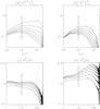 |
Fig. 4 Run B. Turbulence with expansion and no mean field: spectra vs. kR (radial wavenumber, i.e., in direction parallel to the mean radial flow) at t = 0.8,1.2,...3.2 nonlinear times (vertical arrows indicate direction of time evolution). a) Total energy spectra compensated by k− 5/3; b) residual energy, compensated by k-2; c) residual energy |
As observational records by spacecrafts are made along the radial direction, leading via the Taylor hypothesis to 1D reduced spectra versus radial wavenumber, we present only such spectra in Fig. 4, at times t = 0.8, 1.2... 3.2. Total energy spectra are shown compensated by k− 5/3 in panel a, residual spectra are shown compensated by k-2 in panel b. One can thus see in panel a the progressive steepening of the total energy spectrum (starting from the initial 1 /k spectrum) toward a k− 5/3 range and in panel b the formation of the k-2 range for the residual spectrum. Panels c and d show residual spectra normalized by the α = 1 and α = 2 equilibrium spectra, respectively (Eq. (7)). The residual spectra are seen to converge toward the α = 1 model in the inertial range, and much less so toward the α = 2 model.
Magnetic and kinetic spectra also exhibit (not shown) scalings close to 5/3 and 3/2, respectively, but within a wavenumber range that is shorter than for previous run A.
4. Discussion
4.1. The α = 1 model versus simulations and solar wind
Using both compressible MHD and EBM (i.e., compressible MHD modified by expansion) simulations with moderate Mach number, zero mean field, and low cross-helicity, we found that the α = 1 equilibrium between residual and total energy relation (Eq. (7)) holds with the spectra showing the slopes (mT,mR) = (5/3,2) specifically.
We found that in run A the quasi-stationary magnetic spectrum scales as k− 5/3 and the kinetic spectrum scales as k− 3/2; these scalings are observed in the solar wind (Podesta et al. 2007; Salem et al. 2009). This is the first report of this set of slopes in simulations with low cross-correlation in 3D MHD simulations. Previously, the four spectral slopes were found in 2D hybrid simulations by Franci et al. (2015) with the same conditions (no mean field, weak compressibility, and low cross-helicity). Also, incompressible 3D reduced MHD simulations were reported with this set of slopes, but only when forcing with a large cross-helicity (Boldyrev et al. 2011). With no cross-helicity, the latter authors report mR = 2 together with mT = 3/2, which is the prediction of the α = 2 model: this model describes as well the incompressible MG05 simulations. This is discussed again below.
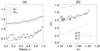 |
Fig. 5 Spectral slopes for total and residual energies: models vs. observations. a) Observations (symbols) as taken from Fig. 5b from Chen et al. (2013) vs. cross-helicity σc; solid line: residual slope as predicted from observed total energy slope using Eq. (16) (α = 1 model). b) Scatter plot (−mT,−mR) from observations (squares); straight lines: relation mR(mT) given in Eq. (9) with α = 0 (dashed line), α = 1 (solid), and α = 2 (dotted). |
The scaling relation associated with the α = 1 model (Eq. (9)), 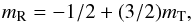 (16)applies well to the average slopes found in the solar wind: mT ≃ 1.7, mR ≃ 2 in the low cross-helicity wind. However, by examining the data published in Chen et al. (2013), in particular their Fig. 5b, we find that the agreement is actually more universal than that. Equation (16) actually also works for cross-helicities σc larger than 0.6, for which the total energy spectrum becomes flatter. This is seen in Fig. 5a, in which we reproduce the measured slopes for total and residual energies versus σc as in Fig. 5b of Chen et al. (2013). The solid line gives the predicted residual slope, replacing the total energy slope by its measured value in Eq. (16). The agreement with the measured mR is seen to increase in the right part of the figure for large cross-helicity, which happens to be the region where error bars are the smallest (see original figure).
Figure 5b summarizes our findings by showing a scatter plot of measured slopes (residual slope versus total energy slope) and comparing these findings with the predictions of the three models for mR(mT): α = 0 (dashed line), 1 (solid), and 2 (dotted). This allows us to see how far from the true situation in the wind are the isotropic edqnm model (α = 2) on the one hand, and the simple α = 0 model.
This indicates that the Alfvén-dynamo theory is able to describe a large interval of turbulent parameters; this theory works in the balanced and imbalanced regime as well with no mean field and average mean field.
4.2. Identifying separately source and damping
To gain more insight into the dynamical process that leads to the α = 1 equilibrium and, in particular, to discriminate between the two possible choices of characteristic times (Eq. (11) or Eq. (12)) that might rule the Alfvén-dynamo equation (Eq. (5)), we now consider the response of the system without expansion (run A) to perturbations of the equilibrium residual energy in two successive experiments.
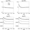 |
Fig. 6 Run A1: return of residual energy to equilibrium after increasing the magnetic energy by a factor four in run A at time t = 10. One-dimensional reduced spectra and time evolution of modes k = 8,16,32 (solid, dotted, and dashed lines, respectively): a) total energy, compensated by k− 5/3; b) residual energy normalized by the α = 1 solution evaluated at time t = 12; c) residual energy and the analytical solution with short damping time (thin lines, cf. Eq. (18) with |
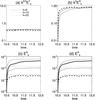 |
Fig. 7 Run A2: return of residual energy to equilibrium after reducing the residual energy to zero by increasing the kinetic energy to the level of magnetic energy. Same caption as in previous figure. |
In both experiments, we restart run A at time t = 10 after perturbing the residual energy spectrum, and follow the evolution up to t = 12. In the first experiment (run A1), we increase the residual energy by increasing the magnetic energy by a factor four at all scales. In the second case (run A2), we decrease the residual energy to zero by raising the kinetic energy to the level of magnetic energy in the whole spectral range. As a result of this procedure, the relative cross-helicity is raised to about 0.4, but still remains below 0.45 up to the end of the run. The progressive relaxation of the system toward equilibrium is shown in Figs. 6 and 7. Panels a and b show the behavior of modes k = 8,16,32 for the total energy compensated by k− 5/3 and for the residual energy normalized by the α = 1 equilibrium. One sees in panels a that the three modes of the total energy remain close together, indicating that the spectral scaling is basically not modified by the perturbation. Panels b show that the three modes of the normalized residual spectrum quickly recover the α = 1 solution in the time lapse 10–12. This occurs within a factor very close to unity in run A1 (Fig. 6) and within a factor ≃0.8 in run A2 (Fig. 7).
Last, we compare the measured numerical relaxation of the residual energy to the analytical solution of the Alfvén-dynamo (Eq. (5)) with α = 1. To this aim, we rewrite Eq. (5), replacing the source term by the equilibrium solution of the α = 1 model,  (17)where
  , and assume the total energy spectrum (as well as the characteristic times and tNL) to be time independent, which is reasonably correct for runs A1 and A2. In practice, we replace these parameters by their value at time t = 12:
 ![Mathematical equation: \hbox{$E^{\rm R}_{\rm eq}(k) = [(t_{\rm A}^0/t_{\rm NL}) E^{\rm T}(k)]_{t=12}$}](/articles/aa/full_html/2016/05/aa28097-16/aa28097-16-eq116.png) . The model solutions thus read
. The model solutions thus read  (18)where either (Eq. (11)) or tD = tNL (Eq. (12)).
In panels c and d we show the model curves (thin lines), where and tD = tNL, respectively, together with the numerical solutions. The agreement for the three modes k = 8,16,32 with the model tD = tNL is clearly much better than with . It is perfect for run A1 (Fig. 6d) and not as good for run A2 (Fig. 7d), but still acceptable; the discrepancy is because the new numerical equilibrium solution is a factor 0.8 smaller than the theoretical equilibrium solution (Eq. (7) with α = 1).
After having validated the (α = 1) equilibrium model in Sect. 3, we have now shown that the relaxation time is tD = tNL. As a consequence, we deduce that the source term in Eq. (5) reads  with , i.e., has the same form as in the edqnm solution. In summary, we proved that the magnetic excess results from the competition between two terms: (i) a slow Alfvén damping with timescale equal to a nonlinear time as predicted by critical balance and (ii) a source term identical to that of the isotropic dynamo found in Grappin et al. (1983) and MG05.
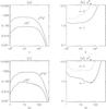 |
Fig. 8 Run C (incompressible MHD, no mean field, MG05). Spectra at time t = 6.5. Top: reduced spectra; Bottom: isotropized spectra. Left: total and residual energy spectra, compensated by k− 5/3 and k-2, respectively. Right: residual energy |
4.3. Incompressible versus compressible simulations
We finally come back on the MG05 incompressible simulations, which we indicated were well described by the α = 2 model, contrary to our compressible simulations that satisfy the α = 1 model. We reexamined the MG05 simulations and found that the origin of the discrepancy lies in the method used to build 1D residual energy spectra. In MG05, the spectra ER(k) were built by averaging the spectral density within spherical shells (later on “isotropized spectra”). In contrast, we used reduced spectra, either ER(kx) (run B) or averages of the three reduced spectra (run A). While we expect that choosing reduced or isotropized spectra matters for run B because expansion introduces a true physical anisotropy in the system (the radial direction becomes a symmetry axis), we expect nothing of the kind without expansion. Indeed, we found that the choice of the spectrum (isotropized or reduced) makes no visible difference in scalings when dealing with runs A, A1, A2 presented here.
However, by reexamining the incompressible MG05 simulations, we found a different situation: residual spectra (but not total energy spectra) present different slopes, depending on whether they are reduced or isotropized. Figure 8 shows spectra for the incompressible run with no mean field considered in MG05 (denoted as run C). Top panels show reduced spectra, bottom panels show isotropized spectra, both at time t = 6.5.
While the total energy spectra show k− 5/3 scalings no matter which spectrum is used, the residual reduced and isotropized spectra show different scalings (compare panels a and c). The reduced residual spectrum scales as k-2 (as do the compressible runs analyzed in the present work), while the isotropized residual spectrum scales as k− 7/3, as reported in MG05. This is confirmed in panels b and d, where we show the residual spectra normalized by the α = 1 (solid lines) and α = 2 (dotted lines) predictions (Eq. (15)). The α = 1 model indeed matches the reduced spectra while the α = 2 model matches the isotropized spectrum, at least qualitatively. This clarifies the problem, but does not solve it; it remains that the incompressible simulations are singular with respect to the measurement of the residual energy spectrum.
4.4. Physical interpretation
We return to the list of different timescales in Eqs. (10)–(13) and forget for a moment that we know which model matches both our numerical (compressible) simulations and observational data. Regarding the damping time tD, the Alfvén effect is clearly at the origin of the damping of the magnetic excess. However, adopting the isotropized Alfvén time  would contradict common wisdom that most of the energy lies in directions perpendicular to the local mean field (Biskamp 2003). Indeed, for the majority of modes at a given scale 1 /k, the effective damping time is not equal to
  but instead to 1/(k∥b0), which, by virtue of the so-called critical balance (Goldreich & Sridhar 1995), is about equal to the nonlinear time tNL: this yields tD = tNL. Now we consider the dynamo time; the simplest choice is clearly tdyn = tNL (Gogoberidze et al. 2012), but since tD = tNL, this would imply that
  , in contradiction with solar wind observations and our numerical evidence.
In contrast, the remaining alternative,  , (together with tD = tNL) matches our numerical data and observations. Thus, the dynamo process responsible for the emergence and sustainment of the observed magnetic excess (~
 ) is not connected with the energy cascade (~ET/tNL) in a straightforward way, as it proceeds on a timescale much longer than the nonlinear time. This is not contradictory to what is known about the dynamo process, which also relies on a (long time) inverse cascade of magnetic helicity. However, this gives a prominent role to the isotropized Alfvén time, in contradiction with the critical balance between the effective Alfvén time and nonlinear time. We presently have no solution for this paradox or for the sensitivity, in incompressible solutions, of the residual spectrum to the definition of the spectrum (isotropized or reduced).
Other attempts to introduce anisotropy into the edqnm equation have made the a priori assumption that the source of the residual spectrum has the same structure as that of the total energy spectrum (Boldyrev et al. 2012). However, again, when applied to our case with no mean field, this assumption
immediately leads to the invalid α = 0 prediction for which mR = mT,  .
.
Several questions remain to be solved and are postponed to future work: (i) why incompressible simulations adopt a singular behavior and (ii) what is the origin of the long timescale tdyn of the local dynamo (Eq. (12)).
Acknowledgments
We thank Simone Landi for interesting discussions. This work was performed using HPC resources from GENCI-IDRIS (grant 2015-040219). A. Verdini acknowledges partial funding from the Interuniversity Attraction Poles Programme initiated by the Belgian Science Policy Office (IAP P7/08 CHARM) and from the European Union’s Seventh Framework Programme for research, technological development, and demonstration under grant agreement No. 284515 (SHOCK, http://project-shock.eu/home/).
References
- Alexakis, A., Mininni, P. D., & Pouquet, A. G. 2005, Phys. Rev. E Stat. Phys., 72, 46301 [NASA ADS] [CrossRef] [Google Scholar]
- Aluie, H., & Eyink, G. L. 2010, Phys. Rev. Lett., 104, 81101 [NASA ADS] [CrossRef] [PubMed] [Google Scholar]
- Biskamp, D. 2003, Magnetohydrodynamic turbulence (Cambridge University Press) [Google Scholar]
- Boldyrev, S., Perez, J. C., Borovsky, J. E., & Podesta, J. J. 2011, ApJ, 741, L19 [NASA ADS] [CrossRef] [Google Scholar]
- Boldyrev, S., Perez, J. C., & Wang, Y.-M. 2012, in Numerical modeling of space plasma flows, 3 [Google Scholar]
- Bruno, R., & Carbone, V. 2013, Liv. Rev. Sol. Phys., 10 [Google Scholar]
- Bruno, R., D’Amicis, R., Bavassano, B., Carbone, V., & Sorriso-Valvo, L. 2007, Ann. Geophys., 25, 1913 [NASA ADS] [CrossRef] [Google Scholar]
- Chen, C. H. K., Bale, S. D., Salem, C. S., & Maruca, B. A. 2013, ApJ, 770, 125 [NASA ADS] [CrossRef] [Google Scholar]
- Dong, Y., Verdini, A., & Grappin, R. 2014, ApJ, 793, 118 [NASA ADS] [CrossRef] [Google Scholar]
- Franci, L., Verdini, A., Matteini, L., Landi, S., & Hellinger, P. 2015, ApJ, 804, L39 [NASA ADS] [CrossRef] [Google Scholar]
- Gogoberidze, G., Chapman, S., & Hnat, B. 2012, Phys. Plasmas, 19, 102310 [NASA ADS] [CrossRef] [Google Scholar]
- Goldreich, P., & Sridhar, S. 1995, ApJ, 438, 763 [NASA ADS] [CrossRef] [Google Scholar]
- Grappin, R., & Velli, M. 1996, J. Geophys. Res., 101, 425 [Google Scholar]
- Grappin, R., Léorat, J., & Pouquet, A. 1983, A&A, 126, 51 [Google Scholar]
- Grappin, R., Velli, M., & Mangeney, A. 1991, Ann. Geophys., 9, 416 [Google Scholar]
- Grappin, R., Velli, M., & Mangeney, A. 1993, Phys. Rev. Lett., 70, 2190 [NASA ADS] [CrossRef] [PubMed] [Google Scholar]
- Kraichnan, R. H. 1965, Phys. Fluids, 8, 1385 [Google Scholar]
- Lee, E., Brachet, M. E., Pouquet, A., Mininni, P. D., & Rosenberg, D. 2010, Phys. Rev. E, 81, 16318 [CrossRef] [Google Scholar]
- Matthaeus, W. H., & Lamkin, S. L. 1986, Phys. Fluids, 29, 2513 [NASA ADS] [CrossRef] [Google Scholar]
- Müller, W.-C., & Grappin, R. 2005, Phys. Rev. Lett., 95, 114502 [NASA ADS] [CrossRef] [Google Scholar]
- Oughton, S., & Matthaeus, W. H. 1995, J. Geophys. Res., 100, 14783 [NASA ADS] [CrossRef] [Google Scholar]
- Podesta, J. J., Roberts, D. A., & Goldstein, M. L. 2007, ApJ, 664, 543 [NASA ADS] [CrossRef] [Google Scholar]
- Roberts, D. A. 1989, J. Geophys. Res., 94, 6899 [Google Scholar]
- Salem, C., Mangeney, A., Bale, S., & Veltri, P. 2009, ApJ, 702, 537 [NASA ADS] [CrossRef] [Google Scholar]
- Stribling, T., & Matthaeus, W. H. 1991, Phys. Fluids B, 3, 1848 [NASA ADS] [CrossRef] [Google Scholar]
- Verdini, A., & Grappin, R. 2015, ApJ, 808, L34 [NASA ADS] [CrossRef] [Google Scholar]
- Zhou, Y., & Matthaeus, W. H. 1990, J. Geophys. Res., 95, 10291 [NASA ADS] [CrossRef] [Google Scholar]
All Figures
|
Fig. 1 Run A (compressible MHD). a) Kinetic (solid line) and magnetic (dotted) rms amplitudes; b) kinetic (solid line) and magnetic (dotted) Taylor wavenumbers vs. time. |
| In the text | |
|
Fig. 2 Run A. Energy spectra averaged during time interval 10 ≤ t ≤ 12. Wavenumbers are normalized by the dissipative wavenumber kd for which k2EM(k) is maximum; see text. a) From top to bottom: total, residual, magnetic, and kinetic energies, compensated resp. by k− 5/3, k-2, k− 5/3, k− 3/2. Spectra are arbitrarily shifted vertically. b) Normalized residual energy |
| In the text | |
|
Fig. 3 Run A. Time variation of spectral energy density at specific wavenumbers k = 4,8,16,32, resp. solid, dotted, dashed, dot-dashed lines. a) Total energy times k5/3b) residual energy times k2; c) residual energy |
| In the text | |
|
Fig. 4 Run B. Turbulence with expansion and no mean field: spectra vs. kR (radial wavenumber, i.e., in direction parallel to the mean radial flow) at t = 0.8,1.2,...3.2 nonlinear times (vertical arrows indicate direction of time evolution). a) Total energy spectra compensated by k− 5/3; b) residual energy, compensated by k-2; c) residual energy |
| In the text | |
|
Fig. 5 Spectral slopes for total and residual energies: models vs. observations. a) Observations (symbols) as taken from Fig. 5b from Chen et al. (2013) vs. cross-helicity σc; solid line: residual slope as predicted from observed total energy slope using Eq. (16) (α = 1 model). b) Scatter plot (−mT,−mR) from observations (squares); straight lines: relation mR(mT) given in Eq. (9) with α = 0 (dashed line), α = 1 (solid), and α = 2 (dotted). |
| In the text | |
|
Fig. 6 Run A1: return of residual energy to equilibrium after increasing the magnetic energy by a factor four in run A at time t = 10. One-dimensional reduced spectra and time evolution of modes k = 8,16,32 (solid, dotted, and dashed lines, respectively): a) total energy, compensated by k− 5/3; b) residual energy normalized by the α = 1 solution evaluated at time t = 12; c) residual energy and the analytical solution with short damping time (thin lines, cf. Eq. (18) with |
| In the text | |
|
Fig. 7 Run A2: return of residual energy to equilibrium after reducing the residual energy to zero by increasing the kinetic energy to the level of magnetic energy. Same caption as in previous figure. |
| In the text | |
|
Fig. 8 Run C (incompressible MHD, no mean field, MG05). Spectra at time t = 6.5. Top: reduced spectra; Bottom: isotropized spectra. Left: total and residual energy spectra, compensated by k− 5/3 and k-2, respectively. Right: residual energy |
| In the text | |
Current usage metrics show cumulative count of Article Views (full-text article views including HTML views, PDF and ePub downloads, according to the available data) and Abstracts Views on Vision4Press platform.
Data correspond to usage on the plateform after 2015. The current usage metrics is available 48-96 hours after online publication and is updated daily on week days.
Initial download of the metrics may take a while.