| Issue |
A&A
Volume 589, May 2016
|
|
|---|---|---|
| Article Number | A20 | |
| Number of page(s) | 7 | |
| Section | Numerical methods and codes | |
| DOI | https://doi.org/10.1051/0004-6361/201527463 | |
| Published online | 06 April 2016 | |
The correct estimate of the probability of false detection of the matched filter in weak-signal detection problems
1
Chip Computers Consulting s.r.l., Viale Don L. Sturzo 82, S.Liberale di
Marcon,
30020
Venice, Italy
e-mail:
This email address is being protected from spambots. You need JavaScript enabled to view it.
2
ESO, Karl Schwarzschild strasse 2, 85748
Garching,
Germany
e-mail:
This email address is being protected from spambots. You need JavaScript enabled to view it.
Received: 28 September 2015
Accepted: 1 February 2016
Abstract
The reliable detection of weak signals is a critical issue in many astronomical contexts and may have severe consequences for determining number counts and luminosity functions, but also for optimizing the use of telescope time in follow-up observations. Because of its optimal properties, one of the most popular and widely-used detection technique is the matched filter (MF). This is a linear filter designed to maximise the detectability of a signal of known structure that is buried in additive Gaussian random noise. In this work we show that in the very common situation where the number and position of the searched signals within a data sequence (e.g. an emission line in a spectrum) or an image (e.g. a point-source in an interferometric map) are unknown, this technique, when applied in its standard form, may severely underestimate the probability of false detection. This is because the correct use of the MF relies upon a priori knowledge of the position of the signal of interest. In the absence of this information, the statistical significance of features that are actually noise is overestimated and detections claimed that are actually spurious. For this reason, we present an alternative method of computing the probability of false detection that is based on the probability density function (PDF) of the peaks of a random field. It is able to provide a correct estimate of the probability of false detection for the one-, two- and three-dimensional case. We apply this technique to a real two-dimensional interferometric map obtained with ALMA.
Key words: methods: statistical / methods: data analysis
© ESO, 2016
1. Introduction
The reliable detection of signals in any observed data is a critical problem common to many subjects (Kay 1998; Tuzlukov 2001; Levy 2008; Macmillan & Creelman 2005). Some specific examples are radar detection (Richards 2005), wireless communication (Zhang 2016), and particle detection (Spieler 2012). In astronomy, this problem arises when looking for faint sources, for instance in the detection of galaxy clusters (Milkeraitis et al. 2010), X-ray point-sources (Stewart 2006), point-sources in the cosmic microwave background (Vio et al. 2004), extra-solar planets (Jenkins et al. 1996), asteroids (Gural et al. 2005), and others. In many practical situations, the technique that is expected to have the best performance, in the sense of providing the greatest probability of true detection for a fixed probability of false detection, is the matched filter (MF). This is the linear filter that maximises the signal-to-noise ratio (S/R) and, therefore, the detectability of the signal of a known structure that is embedded in Gaussian random noise.
This technique, however, is based on the assumption that the position of a signal of interest within a sequence of data (e.g. an emission line in a spectrum) or an image (e.g. a point-source in an interferometric map) is known. Often, in practical application this condition is not satisfied. For this reason, the MF is used assuming that, if present, the position of a signal corresponds to a peak of the filtered data. Here we show that, when based on the standard but wrong assumption that the probability density function (PDF) of the peaks of a Gaussian noise process is a Gaussian, this approach may lead to severely underestimating the probability of false detection. The correct method to accurately compute this quantity is also presented.
In Sect. 2, the main characteristics of MF are reviewed as well as the reason why it provides an underestimate of the probability of false detection. The alternative method to compute this quantity is detailed in Sect. 2.1.3. Finally, in Sect. 3 the procedure is applied to an observed two-dimensional interferometric map that was obtained with ALMA, and the discussion deferred to Sect. 4.
2. Matched filter: an optimal solution of the detection problem
2.1. Mathematical formalization
In this section the basic properties of MF are described. For ease of formalism, arguments will be developed in the context of one-dimensional signals. Extension to higher-dimensional situations is formally trivial and will be briefly highlighted in Sect. 2.1.1.
The detection problem of a one-dimensional deterministic and discrete signal of known structure s = [ s(0),s(1),...,s(N − 1) ] T, with length N, and the symbol T denoting a vector or matrix transpose, is based on the following conditions:
-
1.
The signal of interest has the form s = ag with a a positive scalar quantity (amplitude) and g typically a smooth function often somehow normalized (e.g., max { g(0),g(1),...,g(N − 1) } = 1);
-
2.
The signal is embedded within an additive noise n, i.e. the observed signal x is given by x = s + n. Without loss of generality, it is assumed that E [ n ] = 0, where E [ . ] denotes the expectation operator;
-
3.
The noise n is the realization of a stationary stochastic process with known covariance matrix
![Mathematical equation: \begin{eqnarray} \label{eq:C} \Cb = {E}[\nb \nb^T]. \end{eqnarray}](/articles/aa/full_html/2016/05/aa27463-15/aa27463-15-eq13.png) (1)
(1)
Under these conditions, the detection problem consists of deciding whether x is pure noise n (hypothesis H0) or if it also contains a contribution from a signal s (hypothesis H1). In this way, it is equivalent to a decision problem between the two hypotheses  (2)
(2)
Any decision requires the definition of a criterion and, in this instance, the Neyman-Pearson criterion is an effective choice. It consists of the maximization of the probability of detection PD under the constraint that the probability of false alarm PFA (i.e. the probability of a false detection) does not exceed a fixed value α. According to the Neyman-Pearson theorem (e.g. see Kay 1998), if n is a Gaussian process with covariance function C, ℋ1 has to be chosen when  (3)with
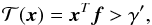
  (4)Here, f is the matched filter. The detection threshold γ for a fixed PFA = α is given by
  (5)where Φ-1(.) is the inverse of the Gaussian complementary cumulative distribution function
  (6)with
  (7)Equation (5)is due to the fact that the statistic
  is a Gaussian random variable with variance sTC-1s and expected value equal to zero under the hypothesis ℋ0, or sTC-1s under the hypothesis ℋ1 (see Fig. 1).
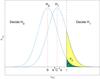 |
Fig. 1 Probability density function of the statistics T(x) under the hypothesis ℋ0 (noise-only hypothesis) and ℋ1 (signal-present hypothesis). The detection-threshold is given by γ. The probability of false alarm (PFA), called also probability of false detection, and the probability of detection (PD) are shown in green and yellow colors, respectively. |
When the threshold γ is fixed, the probability of false detection, α, can be computed by means of ![Mathematical equation: \begin{eqnarray} \label{eq:pfa} \alpha = \Phi \left( \frac{\gamma}{\left[ \ssb^T \Cb^{-1} \ssb \right]^{1/2}} \right)\cdot \end{eqnarray}](/articles/aa/full_html/2016/05/aa27463-15/aa27463-15-eq36.png) (8)For PFA = α, the probability of detection PD is
(8)For PFA = α, the probability of detection PD is 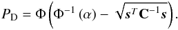 (9)If one sets
 ![Mathematical equation: \begin{eqnarray} \label{eq:MFs} \fb = [0, 0, \ldots, 0, 1, 0, \ldots, 0, 0]^T, \end{eqnarray}](/articles/aa/full_html/2016/05/aa27463-15/aa27463-15-eq39.png) (10)where the only value different from zero is that corresponding to the greatest value of x, the operation (3)becomes a simple thresholding test, which consists of checking if the maximum of the observed data x exceeds a fixed threshold. This simplified version of the MF is adopted in some particular situations (see below).
(10)where the only value different from zero is that corresponding to the greatest value of x, the operation (3)becomes a simple thresholding test, which consists of checking if the maximum of the observed data x exceeds a fixed threshold. This simplified version of the MF is adopted in some particular situations (see below).
2.1.1. Properties of the matched filter
The main characteristics of the MF which are relevant for our discussion are:
-
The extension of MF to the two-dimensional signals
 and
and  is conceptually trivial. Indeed, setting1
![Mathematical equation: \begin{align} \ssb & = {\rm VEC}[\Smatb]; \label{eq:stack1} \\ \xb & = {\rm VEC}[\Xmatb]; \label{eq:stack2} \\ \nb & = {\rm VEC}[\Nmatb], \label{eq:stack3} \end{align}](/articles/aa/full_html/2016/05/aa27463-15/aa27463-15-eq42.png) formally, the problem is the same as the one-dimensional case given by Eq. (2). The only difference is that, in the one-dimensional case, C is a Toeplitz matrix (Antsaklis & Michel 2006) whereas, in the two-dimensional case, it becomes a block Toeplitz with Toeplitz blocks (Ramos et al. 2011) that are difficult to work with. The situation rapidly worsens for higher dimensional cases. Because of this, for problems of dimensionality higher than one, it is preferable to work in the Fourier domain (Kay 1998);
formally, the problem is the same as the one-dimensional case given by Eq. (2). The only difference is that, in the one-dimensional case, C is a Toeplitz matrix (Antsaklis & Michel 2006) whereas, in the two-dimensional case, it becomes a block Toeplitz with Toeplitz blocks (Ramos et al. 2011) that are difficult to work with. The situation rapidly worsens for higher dimensional cases. Because of this, for problems of dimensionality higher than one, it is preferable to work in the Fourier domain (Kay 1998); -
is a sufficient statistic (Kay 1998). Loosely speaking, this means that is able to summarise all the relevant information in the data that concerns the decision described in Eq. (2). No other statistic can perform better;
-
If the amplitude a of the signal is unknown, then the test in Eq. (3) can be rewritten in the form
 (14)where now the MF given by Eq. (4)becomes
  (15)and
 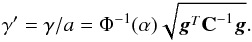 (16)In other words, a statistic independent of a is obtained. For the Neyman-Person theorem, in the case of unknown amplitude of the signal, still maximises PD for a fixed PFA. The only consequence is that PD cannot be evaluated in advance. In principle this can be done a posteriori by using the maximum likelihood estimate of the amplitude,
  ;
; -
In the derivation of Eq. (4), it has been assumed that both x and s have the same length N. This implicitly means that the position of the signal s within the data sequence x is known.
Often, the condition in the last point is not satisfied. In the next section we explore the consequences of this fact.
2.1.2. The application of the matched filter
In real data, the signal of interest s has a length M smaller than the length N of the observed data x (e.g. an emission line in an experimental spectrum). Moreover, often the position of s within the sequence x as well its amplitude a are unknown. In this case the decision problem (2)needs to be modified to  (17)where g(i) is nonzero over the interval [0, M − 1] and i0 is the unknown delay. As a consequence, the statistic in Eq. (3)cannot be applied. The common practice to avoid this problem is based on the following four steps:
-
Computation of the sequence
 through the correlation of x with the MF given by (15)
 (18)This is a linear filtering operation that modifies the characteristics of n. For example, if n has a white-noise spectrum, after the MF operation it becomes coloured (i.e with a non-flat power spectrum);
 -
Determination of the values î0 that maximise
. This operation produces the statistic ![Mathematical equation: \begin{eqnarray} \Tc(\xb, \hat{i}_0) = \underset{ i_0 \in [0, N-M] }{\max} \Tc(\xb, i_0). \end{eqnarray}](/articles/aa/full_html/2016/05/aa27463-15/aa27463-15-eq55.png) (19)Typically,
(19)Typically,  corresponds to the value of the highest peak in ;
 -
A detection is claimed if
 (20)or more commonly, since the quantity gTC-1g can be estimated by means of the sample variance
  of
of  , if
, if  (21)with f given by Eq. (15), and where u is a value in the range [ 3,5 ];
 -
The corresponding probability of false detection is computed by means of
![Mathematical equation: \begin{eqnarray} \label{eq:fd1} \alpha = \Phi \left( \frac{\gamma'}{\left[ \gb^T \Cb^{-1} \gb \right]^{1/2}} \right) \end{eqnarray}](/articles/aa/full_html/2016/05/aa27463-15/aa27463-15-eq64.png) (22)if the test in Eq. (20)is used and
(22)if the test in Eq. (20)is used and  (23)in the other case.
However, the last step is not correct. This is because, with the test (14), we check if at the true position of the hypothetical signal s, the statistic exceeds the detection threshold. Under the hypothesis H0 (i.e. no signal is present in x), there is no reason why such a position must coincide with a peak. Indeed, it corresponds to a generic point of the Gaussian noise process. This is the reason why, as shown in Sect. 2.1, the PDF of is a Gaussian. On the other hand, with the test (20), we check whether the largest peak of exceeds the detection threshold. Now, contrary to the previous case, under the hypothesis H0, the position î0 does not correspond to a generic point of the Gaussian noise process, but rather to the subset of its local maxima. Since the PDF of the local maxima of a Gaussian random process is not a Gaussian, the PDF of cannot be a Gaussian. In other words, the tests (14)and (20)are not equivalent. This problem becomes even more critical if the number of signals of interest is unknown since Steps 3–4 have to be applied to all the peaks in .
2.1.3. A correct computation of the probability of false detection
In a recent paper Cheng & Schwartzman (2015a,b) provide the explicit PDF of the values z of the peaks in a N-dimensional Gaussian isotropic random field of zero-mean and unit-variance for the case N = 1, 2, and 3. For N = 1,  (24)whereas for N = 2
 (25)For the case N = 3, see the original works. Here,
  (26)where ρ′(0) and ρ′′(0) are, respectively, the first and second derivative with respect to r2 of the two-point correlation function ρ(r) at r = 0, with r the inter-point distance. The same authors also provide the expected number Np of peaks per unit area. For N = 1
![Mathematical equation: \begin{eqnarray} E[N_{\rm p}] = \frac{\sqrt{6}}{2 \pi} \sqrt{- \frac{\rho''(0)}{\rho'(0)}}, \end{eqnarray}](/articles/aa/full_html/2016/05/aa27463-15/aa27463-15-eq83.png) (27)whereas for N = 2
(27)whereas for N = 2![Mathematical equation: \begin{eqnarray} \label{eq:number} E[N_{\rm p}] = -\frac{\rho''(0)}{\pi \sqrt{3} \rho'(0)}\cdot \end{eqnarray}](/articles/aa/full_html/2016/05/aa27463-15/aa27463-15-eq84.png) (28)All these equations hold under the condition that ρ(r) be sufficiently smooth and that κ ≤ 1 (see Cheng & Schwartzman 2015a,b).
(28)All these equations hold under the condition that ρ(r) be sufficiently smooth and that κ ≤ 1 (see Cheng & Schwartzman 2015a,b).
On the basis of these results, the probability that a peak due to a zero-mean unit-variance Gaussian noise process exceeds a fixed threshold u can be computed with  (29)
Hence, the fourth step in the above procedure needs to be substituted with
(29)
Hence, the fourth step in the above procedure needs to be substituted with
- 4.
The corresponding probability of false detection is
 (30)
(30)
Figure 2 compares the PDFs ψ(z) for the case N = 2 and κ = 0.5, 0.75, and 1, with the standard Gaussian one. From this figure, the risk of severely overestimating the reliability of a detection is evident. This is supported also by Fig. 3, which shows the ratio Ψ(u)/Φ(u) as a function of the threshold u. For instance, for u = 4, the probability of false detection provided by Φ(u) is about 30 times smaller than that of Ψ(u).
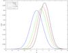 |
Fig. 2 Comparison of the standard Gaussian PDF with those of the peaks of an isotropic two-dimensional zero-mean and unit-variance Gaussian random field when κ = 0.5, 0.75, and 1 (see text). |
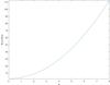 |
Fig. 3 Ratio Ψ(u)/Φ(u) of the two probabilities of false detection for the two cases presented in Sects. 2.1.2 and 2.1.3, as function of the threshold u (see text for details). |
The main problem applying this procedure is the computation of the quantity κ, which in turn requires the knowledge of the analytical form of ρ(r). If the original noise n can be written as n = Hw, with w a white-noise process and H a matrix that implements the discrete form of a known linear filter h(r), then ρ(r) = [h(r) ⊗ f(r)] ⊗ [h(r) ⊗ f(r)] where ⊗ represents the correlation operator, and f(r) the continuous form of the MF (e.g. the theoretical point spread function of the instrument). An alternative method, unavoidable if h(r) is unknown, is to fit the discrete sample two-point correlation function of with an appropriate analytical function. In any case, we have to stress that, as seen above, the knowledge or the estimation of the correlation function of the noise is required also by the MF and, therefore, is not an additional condition of the procedure.
Strictly speaking, the equations above apply only to continuous random fields. However, it is reasonable to expected that they can also be applied with good results to the discrete random fields if ρ(r) is not too “narrow” with respect to the pixel size, or too “wide” with respect to the area spanned by the data. In other words, the correlation length of the random field must be greater than the pixel size and smaller than the data extension. Numerical experiments show that good results are also obtainable when the correlation length is comparable to the pixel size.
If the correlation length is smaller than the pixel size, the resulting random field consists of a discrete white noise and the above equations cannot be applied. Since there is a peak in a discrete random field where the value of a pixel is the greatest among the adjacent ones, the corresponding ψ(z) can be computed using the order statistics (Hogg et al. 2013). For example, in the two-dimensional case ![Mathematical equation: \begin{eqnarray} \label{eq:discrete} \psi(z)= 9 \left[ \Phi(z) \right]^8 \phi(z) \end{eqnarray}](/articles/aa/full_html/2016/05/aa27463-15/aa27463-15-eq106.png) (31)is the PDF of the largest value among nine independent realizations of a zero-mean unit-variance Gaussian process.
(31)is the PDF of the largest value among nine independent realizations of a zero-mean unit-variance Gaussian process.
3. Application to an ALMA observation
We apply the above procedure to extract faint point-sources from a deep map taken with ALMA in Band 6, that targets the Ly-α emitter BDF-3299 (Carniani et al. 2015; Maiolino et al. 2015), and which is shown in Fig. 4a as a 256 × 256 pixel map. The total on-source integration time was roughly 300 min and the reached rms value is 7.8 μJy/beam. The map has been not corrected for the primary beam and, therefore, the resulting noise is uniform across the observed area. We only analyse the central part of the map, as shown in Maiolino et al. (2015), and so it does not cover the entire area that was investigated by these authors.
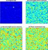 |
Fig. 4 a) original ALMA map; b) original ALMA map with the brightest source removed; c) original ALMA map, standardized to zero-mean and unit-variance, with both the brightest sources removed; d) phase-randomised map (see text). |
A bright source is apparent and, as shown in Fig. 4b, when this is removed and the corresponding area filled with an interpolating two-dimensional cubic spline, another bright source becomes visible. If this is also removed, no additional sources are obvious. In fact, the resulting map in Fig. 4c, standardized to zero-mean and unit-variance, resembles a Gaussian random field. This impression is confirmed by Fig. 5, where the histogram of the pixel values is compared to the standard Gaussian probability density function, as well as by the similarity with Fig. 4d which shows a Gaussian random field, obtained by means of the phase-randomization technique2, which has the same two-dimensional spectrum of the map in Fig. 4c.
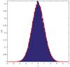 |
Fig. 5 Histogram of the pixel values of the map in Fig. 4c normalized to zero-mean and unit-variance. The red line represents the standard Gaussian probability density function. |
Most of the structures visible in Fig. 4c are certainly not due to physical emission. This means that the question we are faced with is how to detect the point-sources in Gaussian noise which is not, however, white. As seen in Sect. 2, filtering a Gaussian random field that contains a deterministic signal with an MF allows a reduction of the contamination of the unwanted random component and an enhancement of the desired one. In the present case, however, the use of MF is difficult. This is because MF filters out the Fourier frequencies where the noise is predominant, preserving those where the signal of interest gives a greater contribution. However, as shown by Fig. 6, the autocorrelation functions (ACF) along the vertical and the horizontal directions of the brightest object are similar to those of the underlying random field. This means that the point-sources and the blob-shaped structures, which are due to the noise, have similar aspects. In other words, there is nothing to filter out. For this reason, in the first step in the procedure of Sect. 2.1.2 the MF f takes the form (10)and  . Hence, the detection test becomes a thresholding test where a peak in the map is claimed to be a point-source if it exceeds a given threshold.
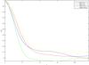 |
Fig. 6 Autocorrelation function along the vertical and the horizontal directions for both the original ALMA map in Fig. 4c and the brightest source visible in Fig. 4a. |
The procedure presented in Sect. 2.1.3 requires the isotropy of the noise field. As shown in Fig. 6 this condition is approximately satisfied. The small differences between the ACFs along the vertical and horizontal directions are probably due to the fact that, as standard procedure for all the interferometric images, the ALMA map in Fig. 4a is the result of a deconvolution (e.g. see Thompson et al. 2004). As is well known, this is a problematic operation. Figure (7)shows that the correlation model 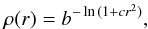 (32)where b and c are free parameters, is able to provide a very good fit to the two-point correlation function of the map. For this model it is
 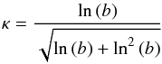 (33)and, in the present case, it results in κ = 0.95. The corresponding PDF for the peaks indicated in Fig. 8 is shown in Fig. 9. Its agreement with the histogram of the peak values is good.
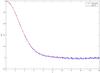 |
Fig. 7 Sample two-point correlation functions for the map in Fig. 4c vs. the fitted one given by Eq. (32). |
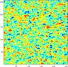 |
Fig. 8 Map of the ALMA Band 6 observations after the removal of the two brightest sources, as shown in Fig. 4c. The small open circles correspond to the identified peaks. |
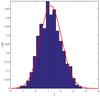 |
Fig. 9 Histograms of the peak values of the maps in Fig. 8, standardized to zero mean and unit variance, vs. the theoretical PDF given by Eq. (25). |
The conclusion is that it is not possible to claim the presence of point-sources, in addition to the two bright ones detected beforehand, because the values of the peaks are compatible with the random fluctuations of a noise field. Indeed, using Eq. (28), the expected number of peaks in the map corresponding to the correlation model (32)is given by ![Mathematical equation: \begin{eqnarray} E[N_{\rm p}] = \frac{c + \ln{b}}{\pi \sqrt{3}} \end{eqnarray}](/articles/aa/full_html/2016/05/aa27463-15/aa27463-15-eq115.png) (34)multiplied by the number of pixels. The result is 822 whereas the number effectively observed is 806. Since the distribution of peaks in the map appears rather regular, this value is well within the ±
(34)multiplied by the number of pixels. The result is 822 whereas the number effectively observed is 806. Since the distribution of peaks in the map appears rather regular, this value is well within the ± interval that is the estimate of the standard deviation for the expected number of points that are generated by a uniform spatial process3. Moreover, the value of the highest peak is zmax = 3.68 and since Ψ(zmax) ≈ 2.62 × 10⁻³, the expected number of peaks that are equal or randomly exceed zmax is 2.62 × 10-3 × 806 ≈ 2, which is a value that is compatible with what has effectively been observed. On the other hand if, following the standard procedure, Φ(zmax) = 1.17 × 10⁻⁴ had been used, the number would be 1.17 × 10-4 × 806 ≈ 10-1. In other words, the peak corresponding to zmax should be considered a detected point-source with a confidence level of 99.99%.
As final comment, we emphasise that these results do not mean that there are only two point-sources in the ALMA map, but only that it is not possible to claim the presence of others at a reliable confidence level.
4. Conclusions
In this paper we show that, when the position and number of the searched signals/sources within observed data are unknown, the commonly-adopted matched filter may severely underestimate the probability of false detection if applied in its standard form. As a consequence, statistical significance can be given to structures that are actually due to the noise. Because of this, an alternative method has been proposed which is able to provide a correct estimate of this quantity. Its application to a map that was taken by ALMA in Band 6 towards a faint extragalactic source demonstrates the risk of spurious detections when the probability of false detection is incorrectly estimated.
VEC [ ℱ ] is the operator that transforms a matrix ℱ into a column array by stacking its columns one underneath the other.
The phase-randomization technique consists in inverting the Fourier spectrum of a map after the substitution of the discrete Fourier phases with uniform random variates in the range [ 0,2π ] (Provenzale et al. 1994).
This term indicates a spatial process that produces a regular distribution of points over an area.
Acknowledgments
This research has been supported by a ESO DGDF Grant 2014 and R.V. thanks ESO for hospitality. The authors thank Stefano Carniani and Roberto Maiolino for providing the ALMA data before publication and for useful discussions, and Andy Biggs for careful reading of the manuscript. This paper makes use of the following ALMA data: ADS/JAO.ALMA#2012.1.00719.S. ALMA is a partnership of ESO (representing its member states), NSF (USA) and NINS (Japan), together with NRC (Canada) and NSC and ASIAA (Taiwan) and KASI (Republic of Korea), in cooperation with the Republic of Chile. The Joint ALMA Observatory is operated by ESO, AUI/NRAO and NAOJ.
References
- Antsaklis, P. J., & Michel, A. N. 2006, Linear Systems (Boston: Birkhäuser) [Google Scholar]
- Carniani, S., Maiolino, R., de Zotti, G., et al. 2015, A&A, 584, A78 [NASA ADS] [CrossRef] [EDP Sciences] [Google Scholar]
- Cheng, D., & Schwartzman, A. 2015a, Extremes, 18, 213 [CrossRef] [Google Scholar]
- Cheng, D., & Schwartzman, A. 2015b, ArXiv e-prints [arXiv:1503.01328] [Google Scholar]
- Gural, P. S., Larsen, J. A., & Gleason, A. E. 2005, AJ, 130, 1951 [NASA ADS] [CrossRef] [Google Scholar]
- Hogg, R. V., McKean, J. W., & Craig, A. T. 2013, Introduction to Mathematical Statistics (New York: Pearson) [Google Scholar]
- Jenkins, J. M., Doyle, L. R., & Cullers, D. K. 1996, Icarus, 119, 244 [NASA ADS] [CrossRef] [Google Scholar]
- Kay, S. M. 1998, Fundamentals of Statistical Signal Processing: Detection Theory (London: Prentice Hall) [Google Scholar]
- Levy, B. C. 2008, Principles of Signal Detection and Parameter Estimation (New York: Springer Science + Business Media) [Google Scholar]
- Maiolino, R., Carniani, S., Fontana, A., et al. 2015, MNRAS, 452, 54 [NASA ADS] [CrossRef] [Google Scholar]
- Macmillan, N. A., & Creelman, C. D. 2005, Detection Theory: a User’s Guide (Mahwah: Lawrence Erlbaum Associates) [Google Scholar]
- Milkeraitis, M., Van Waerbeke, L., Heymans, C., et al. 2010, MNRAS, 406, 673 [NASA ADS] [CrossRef] [Google Scholar]
- Provenzale, A., Vio, R., & Cristiani, S. 1994, ApJ, 428, 591 [NASA ADS] [CrossRef] [Google Scholar]
- Ramos, E. P. R. G., Vio, R., & Andreani, P. 2011, A&A, 528, A75 [NASA ADS] [CrossRef] [EDP Sciences] [Google Scholar]
- Richards, M. A. 2005, Fundamentals of Radar Signal Processing (New York: McGraw-Hill) [Google Scholar]
- Spieler, H. 2012, in Handbook of Particle Detection and Imaging, eds. C. Grupen, & I. Buvat, 53 [Google Scholar]
- Stewart, I. M. 2006, A&A, 454, 997 [Google Scholar]
- Thompson, A. R., Moran, J. M., & Swenson, G. W. 2004, Interferometry and Synthesis in Radio Astronomy (Weiheim: Wiley-VCH) [Google Scholar]
- Tuzlukov, V. P. 2001, Signal Detection Theory (New York: Springer Science + Business Media) [Google Scholar]
- Vio, R., Andreani, P., & Wamsteker, W. 2004, A&A, 414, 17 [NASA ADS] [CrossRef] [EDP Sciences] [Google Scholar]
- Zhang, K. Q. T. 2016, Wireless Communications (Chichester: John Wiley & Sons Ltd) [Google Scholar]
All Figures
|
Fig. 1 Probability density function of the statistics T(x) under the hypothesis ℋ0 (noise-only hypothesis) and ℋ1 (signal-present hypothesis). The detection-threshold is given by γ. The probability of false alarm (PFA), called also probability of false detection, and the probability of detection (PD) are shown in green and yellow colors, respectively. |
| In the text | |
|
Fig. 2 Comparison of the standard Gaussian PDF with those of the peaks of an isotropic two-dimensional zero-mean and unit-variance Gaussian random field when κ = 0.5, 0.75, and 1 (see text). |
| In the text | |
|
Fig. 3 Ratio Ψ(u)/Φ(u) of the two probabilities of false detection for the two cases presented in Sects. 2.1.2 and 2.1.3, as function of the threshold u (see text for details). |
| In the text | |
|
Fig. 4 a) original ALMA map; b) original ALMA map with the brightest source removed; c) original ALMA map, standardized to zero-mean and unit-variance, with both the brightest sources removed; d) phase-randomised map (see text). |
| In the text | |
|
Fig. 5 Histogram of the pixel values of the map in Fig. 4c normalized to zero-mean and unit-variance. The red line represents the standard Gaussian probability density function. |
| In the text | |
|
Fig. 6 Autocorrelation function along the vertical and the horizontal directions for both the original ALMA map in Fig. 4c and the brightest source visible in Fig. 4a. |
| In the text | |
|
Fig. 7 Sample two-point correlation functions for the map in Fig. 4c vs. the fitted one given by Eq. (32). |
| In the text | |
|
Fig. 8 Map of the ALMA Band 6 observations after the removal of the two brightest sources, as shown in Fig. 4c. The small open circles correspond to the identified peaks. |
| In the text | |
|
Fig. 9 Histograms of the peak values of the maps in Fig. 8, standardized to zero mean and unit variance, vs. the theoretical PDF given by Eq. (25). |
| In the text | |
Current usage metrics show cumulative count of Article Views (full-text article views including HTML views, PDF and ePub downloads, according to the available data) and Abstracts Views on Vision4Press platform.
Data correspond to usage on the plateform after 2015. The current usage metrics is available 48-96 hours after online publication and is updated daily on week days.
Initial download of the metrics may take a while.