| Issue |
A&A
Volume 588, April 2016
|
|
|---|---|---|
| Article Number | A147 | |
| Number of page(s) | 7 | |
| Section | Stellar structure and evolution | |
| DOI | https://doi.org/10.1051/0004-6361/201527960 | |
| Published online | 01 April 2016 | |
Mixing of a passive scalar by the instability of a differentially rotating axial pinch
Leibniz-Institut für Astrophysik Potsdam,
An der Sternwarte 16,
14482
Potsdam,
Germany
e-mail: This email address is being protected from spambots. You need JavaScript enabled to view it.
; This email address is being protected from spambots. You need JavaScript enabled to view it.
; This email address is being protected from spambots. You need JavaScript enabled to view it.
Received: 14 December 2015
Accepted: 1 February 2016
Abstract
The mean-field diffusion of passive scalars such as lithium, beryllium or temperature dispersals due to the magnetic Tayler instability of a rotating axial pinch is considered. Our study is carried out within a Taylor-Couette setup for two rotation laws: solid-body quasi-Kepler rotation. The minimum magnetic Prandtl number used is 0.05, and the molecular Schmidt number Sc of the fluid varies between 0.1 and 2. An effective diffusivity coefficient for the mixing is numerically measured by the decay of a prescribed concentration peak located between both cylinder walls. We find that only models with Sc exceeding 0.1 basically provide finite instability-induced diffusivity values. We also find that for quasi-Kepler rotation at a magnetic Mach number Mm ≃ 2, the flow transits from the slow-rotation regime to the fast-rotation regime that is dominated by the Taylor-Proudman theorem. For fixed Reynolds number, the relation between the normalized turbulent diffusivity and the Schmidt number of the fluid is always linear so that also a linear relation between the instability-induced diffusivity and the molecular viscosity results, just in the sense proposed by Schatzman (1977, A&A, 573, 80). The numerical value of the coefficient in this relation reaches a maximum at Mm ≃ 2 and decreases for larger Mm, implying that only toroidal magnetic fields on the order of 1 kG can exist in the solar tachocline.
Key words: instabilities / magnetic fields / diffusion / turbulence / magnetohydrodynamics (MHD)
© ESO, 2016
1. Introduction
Some of the open problems in modern stellar physics are related to empirical findings of rotational periods. Numerical simulations of supernova explosions yield rotation periods of 1 ms for the newborn neutron stars, but the observations provide periods that are much longer. Less compact objects like the white dwarfs are predicted to have equatorial velocities higher than 15 km s-1, but observations show velocities lower than 10 km s-1 (Berger et al. 2005). Obviously, an outward transport of angular momentum occurred, which cannot be explained with the molecular values of the viscosity. Since the cores of the progenitor of newborn neutron stars and white dwarfs are always stably stratified, an alternative instability must exist in the far-developed main-sequence stars, and this transports angular momentum but does not lead to mixing that is too intensive, which seems incompatible with observations of surface abundances in massive stars (Brott et al. 2008).
Even solar observations lead to similar conclusions. The present-day solar core rotates rigidly, but the convection zone still contains lithium, which after a diffusion process between the convection zone and the burning region, 40 000 km under its bottom is destroyed. To explain the lithium decay time of about 1–10 Gyr the effective diffusion coefficient must exceed the molecular viscosity by one or two orders of magnitude. Schatzman (1969, 1977) suggested some sort of instability – appearing in the stably stratified stellar radiation zones – as the generator of this mild extra transport of passive chemicals. For the mixing in the solar model, Lebreton & Maeder (1987) considered a relation D∗ = Re∗ν for the diffusion coefficient (after the notation of Schatzman, see Zahn 1990) with Re∗ ≃ 100. This is a rather low value that leads to D∗ ≲ 103 cm2/s for the solar plasma shortly below the solar tachocline. Brun et al. (1998) worked with Re∗ ≃ 20, while a more refined model of the solar radiative zone starts from the molecular value D ≃ 10 cm2/s and reaches D∗ ≃ 102...4 cm2/s under the influence of a heuristically postulated hydrodynamical instability (Brun et al. 1999).
On the other hand, to reproduce the rigid rotation of the solar interior, the viscosity must exceed its molecular value by more than two orders of magnitude. Rüdiger & Kitchatinov (1996) assume that internal differential rotation interacts with a fossil poloidal magnetic field within the core. The rotation becomes uniform along the field lines. A problem is formed by the “islands” of fast rotation due to the non uniformity of the field lines. A viscosity of more than 104 cm2/s is needed to smooth out such artificial peaks in the resulting rotation laws.
The value of 3 × 104 cm2/s is also reported by Eggenberger et al. (2012) to produce an internal rotation law of the red giant KIC 8366239, which is consistent with the asteroseismological results obtained by the Kepler mission (Beck et al. 2012). Also, Deheuvels et al. (2012, 2014) derive an internal rotation profile of the early red giant KIC 7341231 with a core spinning at least five times faster than the surface. This is less than the stellar evolution codes yield without extra angular momentum transport from the core to the envelope (Ceillier et al. 2012).
That the effective viscosity is more strongly amplified than the effective diffusivity suggests a magnetic background of the phenomena. Magnetic fluctuations transport angular momentum via the Maxwell stress, but they do not transport chemicals. Most sorts of MHD turbulence should thus provide higher eddy viscosity values rather than eddy diffusivity values; this means that both Prandtl numbers and the Schmidt number should exceed unity.
In the present paper, the Tayler instability (Tayler 1957, 1973) in the presence of (differential) rotation is probed to produce diffusion coefficients for passive scalars. By linear theory the instability map is obtained for the unstable nonaxisymmetric mode with m = 1. The eigenvalue problem is formulated for a cylindrical Taylor-Couette container where the gap between both rotating cylinders is filled with a conducting fluid of given magnetic Prandtl number. Inside the cylinders, homogeneous axial electric currents exist that produce an azimuthal magnetic field with the fixed radial profile Bφ ∝ R, which – if strong enough – is unstable even without rotation. It is known that for magnetic Prandtl number of order unity, a rigid rotation strongly suppresses the instability but – as we show – a differential rotation with negative shear destabilizes the flow again so that a wide domain exists in the instability map wherein the nonlinear code provides the spectra of the flow and field fluctuations. Between the rotating cylinders, a steep radial profile for the concentration of a passive scalar is initially established that decays in time by the action of the flow fluctuations. The decay time is then determined in order to find the diffusion coefficient.
2. The rotating pinch
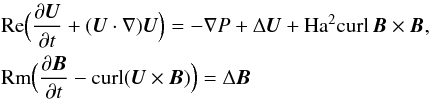
In a Taylor-Couette setup, a fluid with microscopic viscosity ν and magnetic diffusivity η = 1 /μ0σ (σ the electric conductivity) and a homogeneous axial current J = (1 /μ0)curl B are considered. The equations of the system are 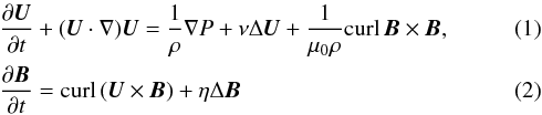 with div U = div B = 0, where U is the actual velocity, B the magnetic field, and P the pressure. Their actual values may be split by
  , and likewise for B and the pressure. The general solution of the stationary and axisymmetric equations is
 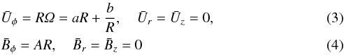 with
with 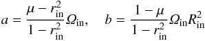 (5)and with A = Bin/Rin. Here, a and b are constants, and A represents the applied electric current. The rotating pinch is formed by a uniform and axial mean-field electric-current. The solutions
  and
and  are governed by the ratios
 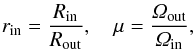 (6)where Rin and Rout are the radii of the inner and the outer cylinders, and Ωin and Ωout are their rotation rates.
Equations (1) and (2) in a dimensionless form become
 (7)and div U = div B = 0. These equations are numerically solved for no-slip boundary conditions and for perfect-conducting cylinders that are unbounded in the axial direction. Those boundary conditions are applied at both Rin and Rout. The dimensionless free parameters in Eqs. (7) are the Hartmann number (Ha) and the Reynolds number (Re),
  (8)where
  is the unit of length and Bin the azimuthal magnetic field at the inner cylinder. With the magnetic Prandtl number,
  (9)the magnetic Reynolds number of the rotation is Rm = Pm Re. For the magnetic Prandtl number of the solar tachocline, Gough (2007) gives the fairly high value Pm ≃ 0.05. There are even smaller numbers down to Pm = 10-4 under discussion (see Brandenburg & Subramanian 2005). However, for the aforementioned red giants, one finds Pm on the order of unity (Rüdiger et al. 2014). The code that solves the equation system (7) is described in Fournier et al. (2005) where the detailed formulation of the possible boundary conditions can also be found. For the present study, only perfectly conducting boundaries have been considered.
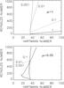 |
Fig. 1 Stability map for m = 1 modes for the pinch with rigid rotation (μ = 1, top panel) and with quasi-Kepler rotation law (μ = 0.35, bottom panel). The critical Hartmann number for resting cylinders is Ha = 35.3 for all Pm. The curves are labeled with their values of Pm, and the curve for Pm = 0.001 represents all curves for smaller Pm. rin = 0.5, perfect-conducting boundaries. |
Figure 1 (top) shows the map of marginal instability for the rigidly rotating pinch with rin = 0.5 and for various Pm. The rotating fluid is unstable in the presence of a magnetic field with parameters on the righthand side of the lines. It also provides the influence of the magnetic Prandtl number on the rotational suppression. The Pm influence completely disappears for the resting pinch with Re = 0. The rotating pinch is massively stabilized for magnetic Prandtl numbers Pm ≥ 0.1. For a very small magnetic Prandtl number, the curves become indistinguishable, meaning that the marginal instability values under the influence of rigid rotation scale with Re and Ha for Pm → 0. This is a standard result for all linear MHD equations in the inductionless approximation for Pm = 0 (if such solutions exist). On the other hand, the rigidly rotating pinch belongs to the configurations with the same radial profiles for velocity (here  ) and magnetic field (here
  ) defined by Chandrasekhar (1956). One can even show that all solutions fulfilling this condition scale with Re and Ha for Pm → 0 (Rüdiger et al. 2015). These facts imply that for a fixed magnetic resistivity, lower molecular viscosities destabilize the rotating pinch.
The situation changes if the two cylinders are no longer rotating with the same angular velocity because the shear energy is now able to excite nonaxisymmetric magnetic instability patterns by interaction with toroidal fields that are current-free within the fluid. In this paper we present the results for the interaction of shear with the azimuthal magnetic field, which is due to the axial electric current, which defines the pinch.
The bottom panel of Fig. 1 gives the instability map for the magnetic instability of a fluid in quasi-Kepler rotation (μ = 0.35) for various Pm. It shows the influence of the differential rotation on the instability map of the rotating pinch. Again, the critical Hartmann number for resting cylinders does not depend on the magnetic Prandtl number, but in addition, the borderlines of the unstable region for all Pm ≤ 1 hardly differ. For the given Reynolds number ranges, the rotational suppression almost disappears for Pm < 1. For Pm = 1 and for Re < 400, the instability becomes even subcritical, and the rotational stabilization changes to a rotational destabilization. For too fast rotation, however, the subcritical excitation disappears, but the rotational suppression is weaker than it is for rigid rotation. According to Fig. 1, the value Pm = 0.1, which is mainly used in the calculations below, already belongs to the small-Pm regime.
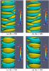 |
Fig. 2 Isolines for the radial component of the velocity in units of ν/D. After the Taylor-Proudman theorem for faster rotation the axial wavelength becomes longer and longer, and the radial rms value of the velocity sinks. Ha = 80, μ = 0.35, Pm = 0.1. |
The flow pattern of the instability is shown in Fig. 2 for quasi-Kepler rotation of growing Reynolds numbers. The Hartmann number is fixed at Ha = 80. The magnetic Mach number of rotation  (10)reflects the rotation rate in units of the Alfvén frequency
  . Almost all cosmical objects possess large magnetic Mach numbers; for example, the white dwarfs rotate with about 2 km s-1, while the observed magnetic field with (say) 1 MG leads to an Alfvén-velocity of about 3 m/s so that Mm ≃ 700. This value even exceeds unity if the largest-ever observed magnetic fields of 100 MG are applied. Inserting the characteristic values for the solar tachocline (R0 = 1.5 × 1010 cm, ρ = 0.2 g/cm3), one finds Mm = 30 /Bφ with Bφ in kG so that with Bφ ≲ 1 kG the tachocline with
  also belongs to the class of rapid rotators. The upper panel of Fig. 1 demonstrates that pinch models with Mm > 1 and rigid rotation are stable, but they easily become unstable if they rotate differentially (see Fig. 1, bottom). This is an important point in the following discussion.
The plots of Fig. 2 represent the radial velocity which basically produces the radial mixing. The instability is nonaxisymmetric, the velocity amplitude does hardly vary for fast rotation but the rms velocity of uR decreases by a factor of 1.6 between Re = 500 and Re = 700, reaching a saturation value, while the axial flow perturbation starts to rise (Fig. 3). Under the influence of fast rotation, a turbulence field that is isotropic in the laboratory system becomes more and more anisotropic, reaching a relation  for the volume-averaged velocity. One finds from Figs. 2 and 3 that the anisotropy – or, in other words, the transition from slow rotation to fast rotation – starts at Re ≈ 600 or Mm ≃ 2, respectively.
This statement is supported by the behavior of the axial wavelength. Within the same interval the axial wavelength – which after the Taylor-Proudman theorem should grow for faster rotation – also seems to jump by the same factor. The question will be whether for Reynolds numbers of about 600 the diffusion coefficient also jumps.
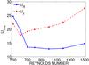 |
Fig. 3 Radial and the axial rms velocity components uR and uz for Mm ≲ 6. Ha = 80, μ = 0.35, Pm = 0.1. |
It is interesting that the estimation uR,rmsL/ 3 for any kind of turbulent diffusivity leads to the maximum value ≈10 ν for the diffusion coefficient. This fairly low value does not fulfill the constraints by Schatzman and Lebreton & Maeder described above. The nonlinear simulations will show whether this preliminary result is confirmed or not.
3. The diffusion equation
For the Tayler unstable system the eddy diffusion of a passive scalar in radial direction is computed. To this end, the additional dimensionless transport equation 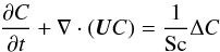 (11)for a passive scalar, C, is added to the equation system (7). This passive scalar can be the temperature or a concentration function of chemicals like lithium or beryllium. Here the microscopic Schmidt number
  (12)is used in Eq. (11), where D is the molecular diffusivity of the fluid. The Schmidt number for gases is of order unity, while it is O(100) for fluids. Gough (2007) gives Sc ≃ 3 with a (radiative) viscosity of 27 cm2/s for the plasma of the solar tachocline. In the present paper, the molecular Schmidt number is varied from Sc = 0.1 to Sc = 2. In their simulations with a driven turbulence probing the Boussinesq type of the diffusion process (Brandenburg et al. 2004) also use Sc = 1 for the molecular Schmidt number.
When the instability is completely developed, it will influence the transport properties of the fluid. This influence might be isotropic or anisotropic, thus different in radial and axial direction. For the latter, Nemri et al. (2012) and Akonur & Lueptow (2002) find a linear dependence between D∗ and Re for the hydrodynamic system with resting outer cylinder. We focus on the radial direction. If D is considered as the molecular diffusivity, its modification can be modeled by an effective diffusivity  (13)where D∗ is only due to the magnetic-induced instability. The goal is to compute the ratio D∗/D as a function of Re and Ha. When averaging Eq. (11) along the toroidal and azimuthal directions, the mean-field value
  follows
  (14)with the effective Schmidt number Sceff = ν/Deff.
To measure the ratio D∗/D, two steps are followed. First, a numerical simulation of Eqs. (7) is performed until the instability is fully developed and energy saturation is reached. The saturation is achieved when the magnetic and kinetic energy of each mode is saturated. Second, the transport Eq. (11) is switched on and several simulations with different Sc numbers are performed. These two steps are repeated for several Re while all other parameters remain fixed.
Since the diffusion leads to a homogenization of the passive scalar profile, the quantity  will exponentially decay in a characteristic time τ that is directly related to the effective Schmidt number. This process will occur whether the magnetic-induced instability is present or not. Two decay times, i.e. τ∗ and τ, will be considered. The first is computed from a simulation where the instability is present and the second from a simulation where evolves alone. Both decay times can be inversely related to their diffusivity, i.e.,
  (15)To compute the decay time, the maximum of the radial profile is plotted at fixed time steps. The characteristic time τ is the e-folding of the resulting profile.
4. Results
Numerical simulations are carried out in a Taylor-Couette container with periodic boundary conditions in the axial direction. Along with the boundary conditions for the velocity and the magnetic field, Neumann boundary conditions at both Rin and Rout are applied for the passive scalar C. To focus on only the radial transport, the initial condition for the passive scalar C0 is chosen to be axisymmetric and constant in the z-direction. These characteristics on C0 will allow the evaluation of the increment on the diffusivity in the radial direction. Thus C0 is taken as a radius-dependent Gaussian centered on the middle of the gap; i.e.,  (16)with r0 = 0.5(Rin + Rout). Since the boundary conditions are periodic in the z-direction and Neumann at cylinder walls, the initial condition will evolve toward a constant profile in the entire cylinder. The maximum of at each time step is plotted, and the characteristic decay time can be computed.
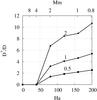 |
Fig. 4 Normalized diffusivity D∗/D vs. the Hartmann number (bottom horizontal axis) and the magnetic Mach number (top horizontal axis). The curves are labeled with the values of the Schmidt number Sc. The value Mm = 1 separates the regimes of slow and fast rotation. Re = 500, μ = 0.35, Pm = 0.1. |
We mainly work with a quasi-Kepler rotation profile that is unstable for the given value of Re = 500 (Fig. 4). The threshold value for the onset of the instability is Ha ≃ 35 from which the value on the effective diffusivity grows. At Ha = 158, the magnetic Mach number Mm becomes unity, defining the regimes of slow rotation (Mm < 1) and fast rotation (Mm > 1). In the slow rotation regime, the normalized diffusivities grow with growing Ha, while they sink with decreasing Ha in the fast rotation regime where the rotation is fast compared to the magnetic field. Figure 4 also demonstrates that D∗/D linearly increases for increasing Sc so that D∗ ∝ ν simply results for Sc > 0.1. It is thus the molecular viscosity alone that determines the diffusion effect of the magnetic-induced instability.
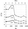 |
Fig. 5 Same as in Fig. 4 but in relation to the Reynolds number (bottom horizontal axis) and the magnetic Mach number (top horizontal axis) for Ha = 80. The value Mm = 1 separates the regimes of slow and fast rotation. Note the reduction of D∗/D for Mm > 2. μ = 0.35, Pm = 0.1. |
The resulting ratio D∗/D for quasi-Kepler rotation and for a fixed Hartmann number is shown in Fig. 5. Now the magnetic Mach number becomes unity at Re = 253. In the slow rotation regime, the effective diffusivity hardly changes. That even without rotation, the ratio D∗/D is different from zero is because the flow is unstable for Re = 0. In the fast rotation regime, the ratio D∗/D increases in a monotonic way until it peaks at about Mm ≃ 2. Finally, for faster rotation (Mm > 2), the effective diffusivity decays due to the rotational quenching. In all cases, however, the effective normalized diffusivity grows with growing Schmidt number so that D∗ ∝ ν also here without any influence from the microscopic diffusivity D. The missing factor in this relation is simply given by the curve for Sc = 1 in Fig. 5.
For all Schmidt numbers, the ratio D∗/D increases monotonically until a certain Re is reached, beyond that it decreases. This behavior can be understood by the ratio D∗/D having to be a direct function of the radial velocity magnitude and the wave number of the solution, since D∗ is produced solely by the instability, which modifies the radial velocity magnitude and the wave number. As shown in Fig. 2, the magnitude of the radial velocity component hardly changes from Re = 400 to Re = 800, while the wavelength increases between Re = 400 and Re = 700. Thus the decreasing of the ratio D∗/D is due to the decrease in the wave number.
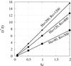 |
Fig. 6 D∗/D as a function of Sc for those Reynolds numbers yielding the maximum instability-induced diffusivities. The magnetic Mach number slightly exceeds 2 in all cases. μ = 0.35, Pm = 0.1. |
Figure 6 shows the normalized diffusivity for μ = 0.35 for fixed Ha as a function of Sc. For all Reynolds numbers, the induced diffusivities D∗ are different from zero, and the ratio D∗/D scales linearly with Sc. The figure only shows the relation for those Reynolds numbers for which the maximum diffusivities for magnetic Mach numbers about 2 are reached. For Sc → 0, the diffusivity D∗ appears to vanish. As a result, for molecular Schmidt numbers Sc > 0.1, the essence of Fig. 6 is the linear relation between D∗/D and Sc. In the notation of Schatzman (1977), it means that  (17)with the scaling factor Re∗ (which indeed forms some kind of Reynolds number). Also, Figs. 4 and 5 demonstrate that linear relations hold for all considered Re and Ha. The Schatzman factor Re∗ after Fig. 6 grows with growing Ha, while for all three models, the magnetic Mach number is nearly the same. We find Re∗ ≲ 4 for Ha = 80 growing to Re∗ ≲ 8 for Ha = 200; a saturation for larger Ha is indicated by the results presented in Fig. 6. It is not yet clear whether for large Ha, an upper limit exists for Re∗ due to numerical limitations.
5. Discussion and conclusions
The influence of the current-induced instability on the effective diffusivity in radial direction of a rotating pinch has been studied for different rotation laws. The diffusion equation is numerically solved in a cylindric setup under the influence of stochastic fluctuations that are due to the magnetic Tayler instability. The conducting fluid between two rotating cylinders becomes unstable if an axial uniform electric current is strong enough. The rotation law between the two cylinders is fixed by their rotation, and our main application is a quasi-Kepler rotation that results when the cylinders are rotating like planets. The magnetic Prandtl number of the fluid is fixed to the value of 0.1, while its Schmidt number (12) is a free parameter of the model.
The main result is a strictly linear relation between the resulting normalized eddy diffusivity D∗/D and the given Schmidt number. The Schatzman relation (17), which also describes our result that for small Schmidt number the eddy diffusivity is negligibly small, has thus been confirmed in a self-consistent way.
The model also provides numerical values for the scaling factor Re∗, which increases for increasing Hartmann number of the toroidal field. For Schmidt numbers ≲0.1, the diffusivity due to the magnetic instability is negligibly small, however Re∗ is different from zero and even exceeds unity in our computations. Already for the value Ha = 80, one finds Re∗ ≲ 4 for quasi-Kepler rotation, and this value increases for increasing Hartmann number (Fig. 6).
The second result concerns the role of the magnetic Mach number Mm which represents the global rotation in relation to the magnetic field strength. For slow rotation, the eddy diffusivity runs linear with Mm, but in all cases a maximum of D∗/D exists at Mm ≃ 2. For faster rotation the induced diffusion is suppressed and finally seems to remain constant (Fig. 5). This fast-rotation phenomenon may be a consequence of the Taylor-Proudman theorem, after which the axial fluctuations are favored at the expense of the radial ones. The correlation lengths in axial direction also grow for growing Reynolds numbers. Both consequences of the Taylor-Proudman theorem appear to retard the growth of the radial diffusion in stars.
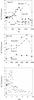 |
Fig. 7 Schatzman number Re∗ vs. Re as functions of Ha (top panel), of Pm (middle panel), and of Mm (bottom panel). In the bottom panel all the simulations of this study are shown. μ = 0.35. |
Figure 7 summarizes the results of this study by presenting numerical values of Re∗ for Kepler rotation laws. In the upper panel, Re∗ is given for four values of the Hartmann numbers as a function of the Reynolds number. Without rotation one finds that Re∗ ∝ Ha is realized, which for solar/stellar Ha-values would produce even higher Re∗-values than the ones found in our computations. With rotation, a maximum of Re∗ exists for approximately one and the same magnetic Mach number (Mm ≃ 2), where the value of Re∗ strongly increases with the Hartmann number. The higher the Hartmann number, the larger Re∗, but this relation is not strictly linear since a mild saturation may exist. For Mm ≫ 2, the rotational quenching leads to Re∗ that is even smaller than the values for Re = 0.
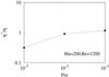 |
Fig. 8 Normalized instability-induced diffusivity η∗/η for the differentially rotating pinch as a function of Pm for the Reynolds and Hartman number, yielding the maximal Re∗. The magnetic Mach number is about 2 (see Fig. 7). μ = 0.35. |
The numerical restrictions of our code prevent calculations for higher Reynolds numbers, but we are able to vary the magnetic Prandtl number. This might be necessary because Pm in the solar tachocline is certainly smaller than 0.1. Figure 7 (middle panel) shows the clear result that Re∗ is anticorrelated with the magnetic Prandtl number. The smaller Pm, the larger Re∗; without rotation, there is even Re∗ ∝ 1 / Pm. For fast rotation, the results do not exclude the possibility that a saturation may occur for Pm ≪ 0.1 so that the influence of Pm becomes weaker as the close lines of marginal instability in Fig. 1 for small Pm suggest.
The bottom panel completes the picture, showing Re∗ as a function of Mm for all simulations used in this study. It shows that Re∗ has a maximum at Mm ≃ 2 and rapidly decreases for large Mm for which it seems to saturate around Re∗ = 1.
A final answer of how large the Schatzman number Re∗ may become by the presented mechanism of nonaxisymmetric instabilities of azimuthal fields cannot be given yet, mainly due to numerical limitations. All the used dimensionless numbers, such as the Reynolds number and the magnetic Mach number, are different from the real (solar) numbers by orders of magnitudes. That the model, proposed in this paper to estimate the magnetic induced extra diffusivity, directly leads to the original formulation of Schatzman seems to be a motivating result. Using the maximal Re∗ values of our curves (which hold for Mm ≃ 2) and by rescaling to the real solar/stellar Hartmann numbers, the resulting Re∗-values would become much too high. The curves in Fig. 7, however, demonstrate a dramatic rotational suppression of the diffusion process for higher Mm so that the low values of Re∗ ≃ 100 that are needed to explain the observations may easily result from the intensive quenching by the global rotation belonging to magnetic Mach numbers exceeding (say) 30. A theoretical explanation of the slow diffusion effects with magnetic instabilities therefore requires differential rotation and weak fields (about a kG), since otherwise the mixing would be too effective.
The presented instability model is based on the simultaneous existence of differential rotation and toroidal magnetic field. It will thus finish after the decay of one of the two ingredients. The question is which of them decays faster by the instability-induced diffusion. Provided the characteristic scales of the differential rotation and the magnetic field are of the same order of magnitude (as is the case for the magnetized Taylor-Couette flows), then the ratio of the decay times of the magnetic field and the differential rotation is  (18)Because the angular momentum transport is also due to the Maxwell stress of the fluctuations, the turbulent viscosity always considerably exceeds the molecular viscosity, which is not the case for the magnetic resistivities for small Pm. We always find that for the rotating pinch, η∗ is on the order of η (Fig. 8). The instability-induced η∗ result from the defining relation, η∗ = ⟨ uφbR − uRbφ ⟩ / 2A of the instability-originated axial component of the electromotive force ⟨ u × b ⟩.
At least for small magnetic Prandtl number, therefore, the instability does not basically accelerate the decay of the fossil magnetic field. As a result, τmag/τrot ∝ (ν∗/ν) Pm. This expression decreases with decreasing magnetic Prandtl number because the normalized turbulent viscosity ν∗/ν also sinks for decreasing Pm for fixed Reynolds number (Rüdiger et al. 2015). For a small magnetic Prandtl number, therefore, the differential rotation never decays faster than the magnetic field, which by itself decays on the long microscopic diffusive timescale. Only for large magnetic Prandtl number might the magnetic angular
momentum transport stop the instability prior to the decay of the fossil field.
Acknowledgments
This work was supported by the Deutsche Forschungsgemeinschaft within the SPP Planetary Magnetism.
References
- Akonur, A., & Lueptow, R. M. 2002, Phys. D, 167, 183 [CrossRef] [Google Scholar]
- Beck, P. G., Montalban, J., & Kallinger, Th. 2012, Nature, 481, 55 [NASA ADS] [CrossRef] [Google Scholar]
- Berger, L., Koester, D., Napiwotzki, R., et al. 2005, A&A, 444, 565 [NASA ADS] [CrossRef] [EDP Sciences] [Google Scholar]
- Brandenburg, A., & Subramanian, K. 2005, Phys. Rep., 417, 1 [NASA ADS] [CrossRef] [Google Scholar]
- Brandenburg, A., Käpylä, P. J., & Mohammed, A. 2004, Phys. Fluids, 16, 1020 [NASA ADS] [CrossRef] [Google Scholar]
- Brott, I., Hunter, I., Anders, P., et al. 2008, AIP Conf. Proc., 990, 273 [NASA ADS] [CrossRef] [Google Scholar]
- Brun, A. S., Turck-Chièze, S., & Morel, P. 1998, ApJ, 506, 913 [NASA ADS] [CrossRef] [Google Scholar]
- Brun, A. S., Turck-Chièze, S., & Zahn, J. P. 1999, ApJ, 525, 1032 [NASA ADS] [CrossRef] [Google Scholar]
- Chandrasekhar, S. 1956, Proc. Natl. Acad. Sci. USA, 42, 273 [NASA ADS] [CrossRef] [Google Scholar]
- Ceillier, T., Eggenberger, T., García, R. A., & Mathis, S. 2012, Astron. Nachr., 333, 971 [NASA ADS] [CrossRef] [Google Scholar]
- Deheuvels, S., Garcia, R., Chaplin, W. J., et al. 2012, ApJ, 756, 19 [NASA ADS] [CrossRef] [Google Scholar]
- Deheuvels, S., Dogan, G., Goupil, M.-J., et al. 2014, A&A, 564, A27 [NASA ADS] [CrossRef] [EDP Sciences] [Google Scholar]
- Eggenberger, P., Montalbán, J., & Miglio, A. 2012, A&A, 544, L4 [NASA ADS] [CrossRef] [EDP Sciences] [Google Scholar]
- Fournier, A., Bunge, H.-P., Hollerbach, R., & Vilotte, J. P. 2005, J. Comput. Phys., 204, 462 [NASA ADS] [CrossRef] [Google Scholar]
- Gough, D. 2007, in The Solar Tachocline, eds. D. Hughes, R. Rosner, & N. Weiss (Cambridge University Press) [Google Scholar]
- Lebreton, Y., & Maeder, A. 1987, A&A, 175, 99 [Google Scholar]
- Nemri, M., Climent, E., Charton, S., Lanoë, J.-Y., & Ode, D. 2012, Chem. Eng. Res. Design, 91, 2346 [CrossRef] [Google Scholar]
- Rüdiger, G., & Kitchatinov, L. L. 1996, ApJ, 466, 1078 [NASA ADS] [CrossRef] [Google Scholar]
- Rüdiger, G., Gellert, M., Schultz, M., et al. 2014, MNRAS, 438, 271 [NASA ADS] [CrossRef] [Google Scholar]
- Rüdiger, G., Schultz, M., Stefani, F., & Mond, M. 2015a, ApJ, 811, 84 [NASA ADS] [CrossRef] [Google Scholar]
- Rüdiger, G., Gellert, M., Spada, F., & Tereshin, I. 2015b, A&A, 573, A80 [NASA ADS] [CrossRef] [EDP Sciences] [Google Scholar]
- Schatzman, E. 1969, Astrophys. Lett., 3, 139 [NASA ADS] [Google Scholar]
- Schatzman, E. 1977, A&A, 56, 211 [NASA ADS] [Google Scholar]
- Tayler, R. J. 1957, Proc. Phys. Soc. B, 70, 31 [NASA ADS] [CrossRef] [Google Scholar]
- Tayler, R. J. 1973, MNRAS, 161, 365 [NASA ADS] [CrossRef] [Google Scholar]
- Zahn, J. P. 1990, in Rotation and Mixing in Stellar Interiors, eds. M.-J. Goupil, & J.-P. Zahn (Springer Verlag), Lect. Notes Phys., 336, 141 [Google Scholar]
All Figures
|
Fig. 1 Stability map for m = 1 modes for the pinch with rigid rotation (μ = 1, top panel) and with quasi-Kepler rotation law (μ = 0.35, bottom panel). The critical Hartmann number for resting cylinders is Ha = 35.3 for all Pm. The curves are labeled with their values of Pm, and the curve for Pm = 0.001 represents all curves for smaller Pm. rin = 0.5, perfect-conducting boundaries. |
| In the text | |
|
Fig. 2 Isolines for the radial component of the velocity in units of ν/D. After the Taylor-Proudman theorem for faster rotation the axial wavelength becomes longer and longer, and the radial rms value of the velocity sinks. Ha = 80, μ = 0.35, Pm = 0.1. |
| In the text | |
|
Fig. 3 Radial and the axial rms velocity components uR and uz for Mm ≲ 6. Ha = 80, μ = 0.35, Pm = 0.1. |
| In the text | |
|
Fig. 4 Normalized diffusivity D∗/D vs. the Hartmann number (bottom horizontal axis) and the magnetic Mach number (top horizontal axis). The curves are labeled with the values of the Schmidt number Sc. The value Mm = 1 separates the regimes of slow and fast rotation. Re = 500, μ = 0.35, Pm = 0.1. |
| In the text | |
|
Fig. 5 Same as in Fig. 4 but in relation to the Reynolds number (bottom horizontal axis) and the magnetic Mach number (top horizontal axis) for Ha = 80. The value Mm = 1 separates the regimes of slow and fast rotation. Note the reduction of D∗/D for Mm > 2. μ = 0.35, Pm = 0.1. |
| In the text | |
|
Fig. 6 D∗/D as a function of Sc for those Reynolds numbers yielding the maximum instability-induced diffusivities. The magnetic Mach number slightly exceeds 2 in all cases. μ = 0.35, Pm = 0.1. |
| In the text | |
|
Fig. 7 Schatzman number Re∗ vs. Re as functions of Ha (top panel), of Pm (middle panel), and of Mm (bottom panel). In the bottom panel all the simulations of this study are shown. μ = 0.35. |
| In the text | |
|
Fig. 8 Normalized instability-induced diffusivity η∗/η for the differentially rotating pinch as a function of Pm for the Reynolds and Hartman number, yielding the maximal Re∗. The magnetic Mach number is about 2 (see Fig. 7). μ = 0.35. |
| In the text | |
Current usage metrics show cumulative count of Article Views (full-text article views including HTML views, PDF and ePub downloads, according to the available data) and Abstracts Views on Vision4Press platform.
Data correspond to usage on the plateform after 2015. The current usage metrics is available 48-96 hours after online publication and is updated daily on week days.
Initial download of the metrics may take a while.