| Issue |
A&A
Volume 588, April 2016
|
|
|---|---|---|
| Article Number | A111 | |
| Number of page(s) | 13 | |
| Section | Interstellar and circumstellar matter | |
| DOI | https://doi.org/10.1051/0004-6361/201527752 | |
| Published online | 28 March 2016 | |
Oxygen, neon, and iron X-ray absorption in the local interstellar medium
1 Max-Planck-Institut für Astrophysik, 85741 Garching bei München, Germany
e-mail: This email address is being protected from spambots. You need JavaScript enabled to view it.
2 Escuela de Física, Facultad de Ciencias, Universidad Central de Venezuela, PO Box 20632, 1020A Caracas, Venezuela
3 Centro de Física, Instituto Venezolano de Investigaciones Científicas (IVIC), PO Box 20632, 1020A Caracas, Venezuela
4 Harvard-Smithsonian Center for Astrophysics, Cambridge, MA, 02138, USA
5 NASA Goddard Space Flight Center, Greenbelt, MD 20771, USA
Received: 16 November 2015
Accepted: 15 February 2016
Abstract
Aims. We present a detailed study of X-ray absorption in the local interstellar medium by analyzing the X-ray spectra of 24 galactic sources obtained with the Chandra High Energy Transmission Grating Spectrometer and the XMM-Newton Reflection Grating Spectrometer.
Methods. By modeling the continuum with a simple broken power-law and by implementing the new ISMabs X-ray absorption model, we have estimated the total H, O, Ne, and Fe column densities towards the observed sources.
Results. We have determined the absorbing material distribution as a function of source distance and galactic latitude–longitude.
Conclusions. Direct estimates of the fractions of neutrally, singly, and doubly ionized species of O, Ne, and Fe reveal the dominance of the cold component, thus indicating an overall low degree of ionization. Our results are expected to be sensitive to the model used to describe the continuum in all sources.
Key words: ISM: general / ISM: atoms / ISM: abundances / ISM: structure / X-rays: ISM
© ESO, 2016
1. Introduction
The interstellar medium (ISM) is one of the most important galactic components. Regarding its chemical composition, it can be enriched with heavy elements by gas accretion from other galaxies, supernova explosions, and stellar winds (Pinto et al. 2013). The analysis of such a dynamic environment is crucial to understand stellar formation and evolutionary processes, which may be performed by means of high-resolution X-ray spectroscopy. Due to their high penetrating power, X-ray photons interact not only with the ISM atomic ions exciting inner-shell levels but also with molecules and solid compounds, thus providing the opportunity to study physical properties such as column densities, ionization fractions, and abundances of astrophysically relevant elements in both the gas and grains (Gatuzz et al. 2015).
Multiple ISM analyses using low-mass X-ray binaries (LMXB) have been carried out in the last decade reporting the presence of a multi-phase ISM structure, which includes a cold gas with low-ionization degree and a hot ionized gas (e.g. Schulz et al. 2002; Takei et al. 2002; Juett et al. 2004; Yao et al. 2009; Liao et al. 2013; Pinto et al. 2013); however, the identification of the highly ionized species is less straightforward than the lowly ionized ones. For example, Gatuzz et al. (2014) performed a study of eight LMXB using high-resolution Chandra spectra, detecting only a Kα absorption feature (22.024 ± 0.003 Å) from highly ionized O vi toward XTE J1817-330. This line was previously identified by Gatuzz et al. (2013a,b) as being intrinsic to the source rather than originating in the local ISM, who concluded that the cold phase is dominant without any further identification of an associated hot gas component. In support of this view, Luo & Fang (2014) have found that most of the absorption lines from highly ionized metals detected in the spectra toward 12 LMXB arise in the hot gas intrinsic to the sources, the ISM only making a small contribution. In a recent study Nicastro (2014) conclude that the absorption line at ~22.275 Å is ubiquitously detected in the spectra of both galactic and extra-galactic sources. It leads to the identification of O ii Kβ from the local ISM thus contradicting its previous identification as an O vi Kα absorption feature of the warm-hot intergalactic medium (WHIM) along the lines of sight toward H 2356–309 (Buote et al. 2009; Fang et al. 2010) and Mkn 501 (Ren et al. 2014).
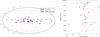 |
Fig. 1 Location map of the X-ray binaries of the present sample. The left panel shows the sources plotted on a full-sky map in galactic coordinates relative to the galactic center. Red points: Chandra sources. Blue points: XMM-Newton sources. The right panel shows a location map of the X-ray binaries in our sample projected in the galactic plane. |
Gatuzz et al. (2013a,b) performed a detailed evaluation of the oxygen absorption region using Chandra high-resolution spectra from the bright binary XTE J1817–330, observing a complex structure around the K edge that included the presence of Kα, Kβ, and Kγ absorption lines from O i and O ii and Kα from O iii, O vi, and O vii. Gatuzz et al. (2014) fitted the O K edge in the Chandra spectra of eight LMXB with the warmabs photoionization model to determine the ISM ionization degree. In this same work, the O photoabsorption cross-section computed by García et al. (2005) was compared with the most recent calculation by Gorczyca et al. (2013), finding no substantial differences in the modeling of the K-shell region; it is worth emphasising the remarkable accuracy of the oxygen atomic data that was thereby established. It was therefore concluded in this work the dominance of a neutral gas in all the observed lines of sight, with ionic fractions O ii/O i and O iii/O i lower than 0.1.
In addition to oxygen, a benchmark of the neon atomic data was also pursued by Gatuzz et al. (2015). Using the high signal-to-noise spectra of Cygnus X–2 and XTE J1817–330, the positions of the Kβ absorption line in Ne i and Kα, Kβ, and Kγ in Ne ii and Ne iii were determined. The Ne i cross-section computed by Gorczyca & McLaughlin (2000) and those for Ne ii and Ne iii by Juett et al. (2006) were adjusted by shifting the wavelength scale in order to fit the astronomical spectra. With the improved cross sections a new X-ray absorption model, referred to as ISMabs, was developed and made publicly available (Gatuzz et al. 2015). Its advantage lies in the compilation of a database of photoabsorption cross sections for neutrally, singly, and doubly ionized species for all the cosmic abundant elements, namely H, He, C, N, O, Ne, Mg, Si, S, Ar, Ca, and Fe. Although the neutral component is dominant in the ISM, it is found that the inclusion of singly and doubly ionized species leads to more realistic models of the O and Ne K edges; furthermore, the use of a physical model prevents misidentification of absorption features which often occurs in the traditional fitting methods with Gaussian profiles.
ISM X-ray absorption affects all the X-ray observations and is particularly evident in high-resolution grating spectra. Even though a careful modeling of the ISM has been previously attempted, its chemical composition and spatial distribution are still under debate (e.g. identification of a galactic highly ionized gas and the existence of a homogeneous distribution at large scales). Moreover, an imprecise ISM modeling can lead to erroneous conclusions when analyzing other environments such as the galactic halo or the WHIM. In this respect, a comprehensive analysis of the ISM through multiple lines of sight and using a realistic absorption model such as ISMabs would be invaluable to address these issues; consequently, we present an extensive analysis of the ISM using XMM-Newton and Chandra high-resolution X-ray spectra.
The outline of this report is as follows. In Sect. 2 the data reduction process is summarised and in Sect. 3 the data fitting procedure is described. A thorough discussion of the results is given in Sect. 4, and finally, we draw in Sect. 5 the conclusions of this work.
2. Observations and data reduction
In order to carry out the present ISM study we have gathered a sample of X-ray binary spectra from the XMM-Newton Science Archive (XSA1) and the Chandra Source Catalog (CSC2). A total of 24 bright sources have been analyzed, 15 from the XSA and 17 from the CSC, some of which have been observed with both telescopes; details of the observations are reviewed in Appendix A. As shown in Fig. 1, the source locations allow an analysis of the ISM along different lines of sight, and it also depicts the source position projected in the galactic plane. The XMM-Newton spectra were reduced with the standard Scientific Analysis System (SAS) threads3 and the Chandra spectra with the standard CIAO threads4. We have estimated the zero-order position for Chandra spectra with the findzo algorithm5. All spectra were rebinned to 25 counts per channel in order to use χ2 statistics. The spectral fitting was performed with the isis data analysis package (Houck & Denicola 2000, version 1.6.2–306).
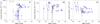 |
Fig. 2 ISMabs column densities for Chandra observations as a function of the number of counts. Black points correspond to Chandra TE-mode spectra and blue points to Chandra CC-mode spectra. |
ISMabs column density values.
3. Spectral fitting procedure
In order to estimate the O, Ne, and Fe column densities we have carried out a broadband fit (11–24 Å) for each source listed in Appendix A using a simple ISMabs*Bknpower model. The Bknpower component corresponds to a broken power-law that in general provides a better fit to the continuum than a single unbroken power-law. In the case of Sco X–1, we analysed the spectra in the 15–24 Å region due to the absence of data below this wavelength range. The ISMabs model (Gatuzz et al. 2015) includes photoabsorption cross sections for neutrally, singly, and doubly ionized species, and the Fe photoabsorption cross-section is taken from metallic iron laboratory measurements (Kortright & Kim 2000). For each source all observations were fitted simultaneously (i.e. using the same absorption parameters and varying the normalisation for each observation); in the case of Chandra, we considered observations with timed exposure (TE) readout mode and continuous clocking (CC) readout mode separately. The free parameters for the ISMabs fits were the H, O, Ne, and Fe column densities, including the O ii, O iii, Ne ii, and Ne iii ions.
Data statistics (e.g. number of counts in the wavelength region of interest) clearly have a significant impact on the absorption modeling. Figure 2 shows the ISMabs column densities obtained from the Chandra observations as function of the number of counts in the O (21–24 Å), Ne (13–15 Å), and Fe (16–18 Å) absorption regions, which brings out a disparity in the O columns when the number of counts is low. This is probably due to the fact that in the CC read mode the details of the spatial distribution are lost, and therefore, there is no way to spatially separate the background from the source. This affects the spectra at long wavelengths where the effective area is smaller and where the background may become comparable to the source signal.
Specifically, CC-mode observations with less than approximately 2000 counts in the O K-edge region give rise to the outliers in the left panel of Fig. 2. Therefore, in the following procedures we excluded observations with a limited number of counts in the O K-edge region (21–24 Å) and Ne K-edge region (13–15 Å). Additional information on the influence of Chandra readout modes in high-resolution spectroscopy are given in Appendix B. Finally, for those sources with observations from both Chandra and XMM-Newton, we have found that the derived columns are in good agreement and, therefore, we take the average of the fit values.
4. Results and discussions
Fit results to all the observations in our sample are listed in Table 1. Upper limits for the column densities (i.e. the highest values obtained for each ion considering their upper errors) in units of 1017 cm-2 are: N(O I) < 32.46; N(O II) < 2.55; N(O III) < 3.37; N(Ne I) < 10.95; N(Ne II) < 2.11; N(Ne III) < 0.20; and N(Fe) < 2.31. Figure 3 shows the column density distribution for each source. The hydrogen and neon column densities are mostly consistent and are homogeneously distributed along their average value; this is expected in neon since it does not form molecules. Oxygen and iron column densities, on the other hand, tend to be more dispersed along the different lines of sight. This is further discussed in Sect. 4.3.
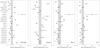 |
Fig. 3 ISMabs column densities values for each source. Gray boxes correspond to a 2σ region around the average value. |
Hydrogen column density comparison.
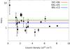 |
Fig. 4 Comparison of hydrogen column densities from different 21 cm surveys with the present ISMabs results. Black data points corresponds to the ISMabs/21 cm ratio using the Dickey & Lockman (1990) measurements. The solid color lines are linear fits to the ISMabs/21 cm values relative to the various determinations from the 21 cm surveys: Dickey & Lockman (1990, red line), Kalberla et al. (2005, green line) and Willingale et al. (2013, blue line). |
4.1. Hydrogen column densities
A comparison of the ISMabs hydrogen column densities with the data sets from the 21 cm surveys (Dickey & Lockman 1990; Kalberla et al. 2005; Willingale et al. 2013) is provided in Table 2. The 21 cm hydrogen column densities correspond to the average value of all absorbers within 1° of the source position. It is important to note that Dickey & Lockman (1990) and Kalberla et al. (2005) only consider the atomic H i column density while Willingale et al. (2013) includes both atomic and molecular hydrogen. Figure 4 shows a comparison of the 21 cm measurements with those derived from our ISMabs fits. Black data points corresponds to the ISMabs/21 cm ratio using the Dickey & Lockman (1990) measurements. The solid color lines are linear fits to the ISMabs/21 cm values relative to the various determinations from the 21 cm surveys (Dickey & Lockman 1990; Kalberla et al. 2005; Willingale et al. 2013). For low column densities the ISMabs values tend to be systematically larger than the 21 cm values while for high column densities the ISMabs values tend to be lower than the 21 cm values. We found overall that the best agreement of our results is with those from Willingale et al. (2013).
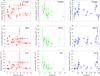 |
Fig. 5 Comparison of the oxygen, neon, and iron total column densities obtained from the ISMabs model as function of distance (left panels), latitude absolute value (middle panels), and longitude (right panels) for all the analysed sources. Longitude has been rescaled to 0°−180°. |
These discrepancies may arise from either a real difference in the intrinsic absorption or the continuum model; also, changes in the region around the X-ray source due to changes in the intrinsic column (e.g. the presence of winds) can increase absorption, and they are thus not resolved by the 21 cm surveys. These effects are more likely to be important in sources with strong stellar winds such as Cyg X–1 and Sco X–1 (Gatuzz et al. 2014). On the other hand, the hydrogen column densities obtained from broadband fits are subject to the uncertainty of the assumed underlying continuum. In some cases, the description of the spectra with different models such as Powerlaw, Bknpower, and Blackbody leads to differences in the column densities despite similar statistics. Therefore, since we are not able to favor a continuum model based on fit statistics, we have adopted for consistency and simplicity the Bknpower model for all observations. We emphasise that the continuum model must be treated carefully in any attempt to perform an ISM analysis with X-ray high-resolution spectroscopy. In this respect our results are expected to be sensitive to the particular model used to describe the continuum in all sources.
4.2. ISM structure
Figure 5 shows a comparison of the oxygen, neon, and iron total column densities from the ISMabs model as a function of distance (left panels), latitude absolute value (central panels), and longitude (right panels) for all the analysed sources. We have found that the column densities tend to increase with distance, the slope being steeper in the case of oxygen, and the general trend is to decrease with galactic latitude. This behavior is expected because the ISM material density decreases along the vertical direction away from the galactic plane. In the case of galactic longitude, it is difficult to establish a clear relationship with the column density but an increase at high longitude (i.e. away from the galactic center) is hinted.
We have derived the column-density unweighted average considering all individual sources, namely (in units of 1017 cm-2) N(O) = 18.43 ± 2.53, N(Ne) = 4.91 ± 1.19, and N(Fe) = 0.90 ± 0.18. Using the total column densities for each element, we have estimated elemental abundances with the relation Nx = AxNh, where Nh is the hydrogen column density, Ax is the abundance, and Nx is the total column density of element x; the resulting values are listed in Table 3. The abundance behavior, in the other hand, tend to be constant with distance and latitude; regarding longitude, sources with high hydrogen column densities tend to have increased abundances at low longitude values. Using the abundance values computed for all individual sources, we have derived unweighted average values relative to solar (Grevesse & Sauval 1998) of AO = 0.70 ± 0.26, ANe = 0.87 ± 0.35, and AFe = 0.67 ± 0.28.
The comparison of the oxygen and iron total column densities as a function of the neon column density is shown in Fig. 6, including for each element contributions from the neutrally, singly, and doubly ionized species. The best fitted Nx/NNe abundance ratio for all sources is plotted with the solid red line; ratios from Grevesse & Sauval (1998), Asplund et al. (2009), Lodders et al. (2009) and Juett et al. (2004) are also shown. Neon, being a noble gas, is a suitable baseline since it is only found in atomic form. We find an average ratio of N(O) /N(Ne) = 4.16 ± 0.22 larger than the estimate by Juett et al. (2006) of 3.7 ± 0.3 and lower than the solar values of 4.79 (Lodders et al. 2009), 5.36 (Grevesse & Sauval 1998) and 5.75 (Asplund et al. 2009). We also obtain an average ratio of N(Fe) /N(Ne) = 0.18 ± 0.01 in relatively close agreement with Juett et al. (2006) (0.15 ± 0.01) and lower than the solar ratios by Grevesse & Sauval (1998), Lodders et al. (2009) and Asplund et al. (2009) of 0.26, 0.25 and 0.37, respectively.
Abundance values.
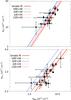 |
Fig. 6 Comparison of the abundance ratios NO/NNe (top panel) and NFe/NNe (bottom panel) obtained from the broadband fit with ISMabs for all the analysed sources. The best fitted Nx/NNe ratio for all sources is plotted with a solid red line. Ratios obtained from Grevesse & Sauval (1998), Asplund et al. (2009), Lodders et al. (2009) and Juett et al. (2004) are respectively shown with green, blue, orange and magenta dashed lines. |
The presence of ionized species in the ISM is not negligible and must be considered in order to perform a reliable chemical analysis of its environment. Figure 7 shows a comparison of the O ii/O i, O iii/O i, Ne ii/Ne i, and Ne iii/Ne i ionization fractions as function of distance, latitude absolute value, and longitude. Unlike the column densities, the ionization fractions tend to be approximately constant with the geometric parameters. This result agrees with previous findings regarding the dominance of the ISM cold phase characterized by a low ionization degree (Gatuzz et al. 2013a,b, 2014, 2015). We obtained the following average values: O ii/O i= 0.03 ± 0.01; O iii/O i= 0.03 ± 0.02; Ne ii/Ne i= 0.21 ± 0.05; and Ne iii/Ne i= 0.03 ± 0.02.
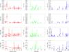 |
Fig. 7 Comparison of the ionization fractions O ii/O i, O iii/O i, Ne ii/Ne i, and Ne iii/Ne i obtained with the ISMabs model as function of distance (left panels), the latitude absolute value (middle panels), and longitude (right panels) for all the analysed sources. Longitude has been rescaled to 0°−180°. |
4.3. Molecular absorption features
The search for molecular and dust spectral signatures is a topic of current interest in ISM astrophysics. Lee et al. (2009) argued that Chandra and XMM-Newton high-resolution spectra provide a resource to constrain dust properties (e.g. distribution, composition, and abundances). Absorption features due to molecules and dust have been studied previously using LMXB (de Vries & Costantini 2009; Kaastra et al. 2009; Pinto et al. 2010; Costantini et al. 2012; Pinto et al. 2013); in particular, de Vries & Costantini (2009) estimated an oxygen depletion rate to the solid state of 30−50% from an XMM-Newton RGS spectrum of Sco X–1. However, García et al. (2011) showed that, by taking into account an improved photoabsorption cross section for atomic oxygen which takes into account Auger damping, the same observation could be adequately modelled without invoking molecular or dust contributions. The best X-ray absorption model should include both atomic and molecular cross sections. However, since the spectral features from solid compounds are expected to be weak, an accurate modeling of the atomic components is a prerequisite.
In this respect, Pinto et al. (2010) previously analysed XMM-Newton spectra of the binary GS 1826–238, and after modeling the atomic component, they included molecular and dust contributions to diminish the high residuals near the oxygen edge. They derived column densities for andradite (Ca3Fe2Si3O12), amorphous ice (H2O), carbon monoxide (CO), and hercynite (FeAl2O4); however, their model included the same undamped atomic cross sections used in previous studies. Figure 8 shows XMM-Newton spectra of GS 1826–238 in the 21–24 Å region modeled by ISMabs, which takes into account a more recent and Auger-damped atomic cross section. Although ISMabs includes neither molecular nor solid photoabsorption cross-sections, it leads to a good fit of the O K-edge absorption features with well-distributed small residuals; that is, the apparent lack of absorption previously perceived by Pinto et al. (2010) was due, in our opinion, to a poor atomic model. Our results imply an upper limit to the amount of oxygen which can be in molecular or solid form. A quantitative estimate for this limit requires simultaneous fits using both our accurate atomic oxygen K shell cross sections and the best available models for absorption by molecules and dust. This will be the subject of future investigations.
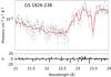 |
Fig. 8 GS 1826–238 XMM-Newton spectra in the oxygen K-edge region. Observations were combined for illustrative purposes. |
It is important to note that, since the valence electronic levels of molecules or dust are more fully occupied than those of atoms, the Kα resonance lines from molecules and dust will in general be weaker than atoms, or absent. Thus, the addition of molecules or dust to an atomic model when fitting to observed ISM X-ray spectra will lead to a larger ratio of edge to line. Our fits do not show a systematic discrepancy or statistically significant errors in this ratio, thus reinforcing the conclusion that molecules and grains are a minor contributor to the absorption in the spectral region near the oxygen K edge.
5. Conclusions
We have performed a thorough analysis of the ISM along 24 lines of sight by means of high-resolution X-ray spectroscopy with spectra obtained from both the Chandra and XMM-Newton space observatories. This is the most complete study to date of this type and considering O and Ne charge states. We have found that data statistics (i.e. number of counts for a given wavelength region) has a sizeable impact on the analysis, which is particularly important in the case of Chandra observations taken in CC-mode as they require a higher number of counts than those in TE-mode in order to avoid background contamination. For sources observed with both telescopes, the derived column densities are in good agreement and thus average values are listed.
Using the ISMabs X-ray absorption model, we have obtained upper limits for the column densities of H i, O i, O ii, O iii, Ne i, Ne ii, Ne iii, and metallic Fe. In the case of hydrogen, we found differences between our fits and the 21 cm surveys. These discrepancies may arise from intrinsic absorption variabilities in each source as well as the particular choice of continuum representation. Our measurements indicate an increase of the column densities with source distance and a decrease with galactic latitude. We find that the ionization fractions, on the contrary, tend to be constant with distance and latitude reinforcing previous conclusions regarding the dominance of the neutral ISM component.
We have also derived the N(O) /N(Ne) and N(Fe) /N(Ne) abundance ratios finding lower values than solar (Grevesse & Sauval 1998). Using the total column densities, we estimate the O, Ne, and Fe abundances to be, respectively, ~70%, ~87%, and ~67% relative to the solar standards of Grevesse & Sauval (1998) and ~97%, ~122%, and Fe ~67% relative to the revised values of Asplund et al. (2009). In general, the abundances show a trend different to that observed in the column densities: they tend to be constant with distance and latitude.
It is important to note that this study only considers a small fraction of the local ISM environment due to the lack of a larger database of bright LMXB to perform a more extensive analysis. Observations with new-generation instrumentation such as Astro-H will allow a finer examination of the ISM large structures. The present work will be followed by a search and study of molecular and dust absorption features.
Note added in proof. While this paper was in review an X-ray analysis of the Galactic ISM was published (Nicastro et al. 2016). We agree with their findings on the presence of both a cold neutral component, dominated by O I, and a warm midly ionized component, which contains O I and O II.
References
- Asplund, M., Grevesse, N., Sauval, A. J., & Scott, P. 2009, ARA&A, 47, 481 [NASA ADS] [CrossRef] [Google Scholar]
- Buote, D. A., Zappacosta, L., Fang, T., et al. 2009, ApJ, 695, 1351 [NASA ADS] [CrossRef] [Google Scholar]
- Costantini, E., Pinto, C., Kaastra, J. S., et al. 2012, A&A, 539, A32 [NASA ADS] [CrossRef] [EDP Sciences] [Google Scholar]
- de Vries, C. P., & Costantini, E. 2009, A&A, 497, 393 [NASA ADS] [CrossRef] [EDP Sciences] [Google Scholar]
- Dickey, J. M., & Lockman, F. J. 1990, ARA&A, 28, 215 [NASA ADS] [CrossRef] [MathSciNet] [Google Scholar]
- Fang, T., Buote, D. A., Humphrey, P. J., et al. 2010, ApJ, 714, 1715 [NASA ADS] [CrossRef] [Google Scholar]
- Galloway, D. K., Muno, M. P., Hartman, J. M., Psaltis, D., & Chakrabarty, D. 2008, ApJS, 179, 360 [NASA ADS] [CrossRef] [Google Scholar]
- García, J., Mendoza, C., Bautista, M. A., et al. 2005, ApJS, 158, 68 [NASA ADS] [CrossRef] [Google Scholar]
- García, J., Ramírez, J. M., Kallman, T. R., et al. 2011, ApJ, 731, L15 [NASA ADS] [CrossRef] [Google Scholar]
- Gatuzz, E., García, J., Mendoza, C., et al. 2013a, ApJ, 778, 83 [NASA ADS] [CrossRef] [Google Scholar]
- Gatuzz, E., García, J., Mendoza, C., et al. 2013b, ApJ, 768, 60 [NASA ADS] [CrossRef] [Google Scholar]
- Gatuzz, E., García, J., Mendoza, C., et al. 2014, ApJ, 790, 131 [NASA ADS] [CrossRef] [Google Scholar]
- Gatuzz, E., García, J., Kallman, T. R., Mendoza, C., & Gorczyca, T. W. 2015, ApJ, 800, 29 [NASA ADS] [CrossRef] [Google Scholar]
- Gorczyca, T. W., & McLaughlin, B. M. 2000, J. Phys. B: At. Mol. Opt. Phys., 33, L859 [NASA ADS] [CrossRef] [Google Scholar]
- Gorczyca, T. W., Bautista, M. A., Hasoglu, M. F., et al. 2013, ApJ, 779, 78 [NASA ADS] [CrossRef] [Google Scholar]
- Grevesse, N., & Sauval, A. J. 1998, Space Sci. Rev., 85, 161 [NASA ADS] [CrossRef] [Google Scholar]
- Grimm, H.-J., Gilfanov, M., & Sunyaev, R. 2002, A&A, 391, 923 [NASA ADS] [CrossRef] [EDP Sciences] [Google Scholar]
- Houck, J. C., & Denicola, L. A. 2000, in Astronomical Data Analysis Software and Systems IX, eds. N. Manset, C. Veillet, & D. Crabtree, ASP Conf. Ser., 216, 591 [Google Scholar]
- Hynes, R. I., Steeghs, D., Casares, J., Charles, P. A., & O’Brien, K. 2004, ApJ, 609, 317 [NASA ADS] [CrossRef] [Google Scholar]
- in’t Zand, J. J. M., Kuulkers, E., Verbunt, F., Heise, J., & Cornelisse, R. 2003, A&A, 411, L487 [NASA ADS] [CrossRef] [EDP Sciences] [Google Scholar]
- Jonker, P. G., & Nelemans, G. 2004, MNRAS, 354, 355 [NASA ADS] [CrossRef] [Google Scholar]
- Juett, A. M., Schulz, N. S., & Chakrabarty, D. 2004, ApJ, 612, 308 [NASA ADS] [CrossRef] [Google Scholar]
- Juett, A. M., Schulz, N. S., Chakrabarty, D., & Gorczyca, T. W. 2006, ApJ, 648, 1066 [NASA ADS] [CrossRef] [Google Scholar]
- Kaastra, J. S., de Vries, C. P., Costantini, E., & den Herder, J. W. A. 2009, A&A, 497, 291 [NASA ADS] [CrossRef] [EDP Sciences] [Google Scholar]
- Kalberla, P. M. W., Burton, W. B., Hartmann, D., et al. 2005, A&A, 440, 775 [NASA ADS] [CrossRef] [EDP Sciences] [Google Scholar]
- Kortright, J. B., & Kim, S.-K. 2000, Phys. Rev. B, 62, 12216 [NASA ADS] [CrossRef] [Google Scholar]
- Kuulkers, E., den Hartog, P. R., in’t Zand, J. J. M., et al. 2003, A&A, 399, 663 [NASA ADS] [CrossRef] [EDP Sciences] [Google Scholar]
- Lee, J. C., Xiang, J., Ravel, B., Kortright, J., & Flanagan, K. 2009, ApJ, 702, 970 [NASA ADS] [CrossRef] [Google Scholar]
- Liao, J.-Y., Zhang, S.-N., & Yao, Y. 2013, ApJ, 774, 116 [NASA ADS] [CrossRef] [Google Scholar]
- Lodders, K., Palme, H., & Gail, H.-P. 2009, in Landolt Börnstein, Vol. VI/4B, 560 [Google Scholar]
- Luo, Y., & Fang, T. 2014, ApJ, 780, 170 [NASA ADS] [CrossRef] [Google Scholar]
- Nicastro, F. 2014, in The X-ray Universe 2014, ed. J.-U. Ness, 11 [Google Scholar]
- Nicastro, F., Senatore, F., Gupta, A., et al. 2016, MNRAS, 457, 676 [NASA ADS] [CrossRef] [Google Scholar]
- Paerels, F., Brinkman, A. C., van der Meer, R. L. J., et al. 2001, ApJ, 546, 338 [NASA ADS] [CrossRef] [Google Scholar]
- Pinto, C., Kaastra, J. S., Costantini, E., & Verbunt, F. 2010, A&A, 521, A79 [NASA ADS] [CrossRef] [EDP Sciences] [Google Scholar]
- Pinto, C., Kaastra, J. S., Costantini, E., & de Vries, C. 2013, A&A, 551, A25 [NASA ADS] [CrossRef] [EDP Sciences] [Google Scholar]
- Ren, B., Fang, T., & Buote, D. A. 2014, ApJ, 782, L6 [NASA ADS] [CrossRef] [Google Scholar]
- Sala, G., & Greiner, J. 2006, ATel, 791, 1 [NASA ADS] [Google Scholar]
- Schulz, N. S., Cui, W., Canizares, C. R., et al. 2002, ApJ, 565, 1141 [NASA ADS] [CrossRef] [Google Scholar]
- Takei, Y., Fujimoto, R., Mitsuda, K., & Onaka, T. 2002, ApJ, 581, 307 [NASA ADS] [CrossRef] [Google Scholar]
- Willingale, R., Starling, R. L. C., Beardmore, A. P., Tanvir, N. R., & O’Brien, P. T. 2013, MNRAS, 431, 394 [NASA ADS] [CrossRef] [Google Scholar]
- Yao, Y., Schulz, N. S., Gu, M. F., Nowak, M. A., & Canizares, C. R. 2009, ApJ, 696, 1418 [NASA ADS] [CrossRef] [Google Scholar]
- Ziółkowski, J. 2005, MNRAS, 358, 851 [NASA ADS] [CrossRef] [Google Scholar]
Appendix A: Data sample
Chandra observation list.
For this analysis we use a sample of 84 observations; the details of the Chandra and XMM-Newton observations are listed in Tables A.1, A.2. The number of counts for each observation in the broadband fit region (11–24 Å), O K-edge region (21–24 Å), Ne K-edge region (13–15 Å), and Fe L-edge region (16–18 Å) are also included. In the case of Chandra, 20 and 29 observations were taken in TE-mode and CC-mode, respectively.
XMM-Newton observation list.
Figures A.1, A.2 show the best broadband fit for each source in flux units. In cases where more than one observation is present, the observations are fitted simultaneously varying the continuum parameters and have been onlycombined for illustrative purposes. The best-fit model is indicated by a solid red line. In the case of Sco X–1, the broadband fit was performed in the 15–24 Å wavelength range due to the absence of data below 15 Å (see Fig. A.3). The dominant observed absorption features correspond to the O K edge (~23 Å), Ne K edge (~14 Å), Fe L edge (~17 Å), and the O i Kα transition (~23.5 Å). In general, a smooth residual distribution (bottom panels) around these edges is observed, indicating modeling accuracy that relies on the most up-to-date atomic data. It must be emphasised that the absence of molecular photoabsorption cross-sections in the ISMabs model (except for metallic Fe) does not represent a spectral fitting limitation. This issue has been discussed in Sect. 4.3. All data have been rebinned to 25 counts per channel and combined for illustrative purposes
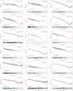 |
Fig. A.1 ISMabs best broadband fits for the analysed sources where observations are combined for illustrative purposes. In the case of Chandra the read mode (CC-mode or TE-mode) is indicated. |
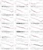 |
Fig. A.2 ISMabs best broadband fits for the analysed sources where observations are combined for illustrative purposes. In the case of Chandra the read mode (CC-mode or TE-mode) is indicated. |
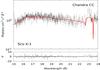 |
Fig. A.3 ISMabs best broadband fits for Sco X-1. Observations were combined for illustrative purposes. |
Appendix B: Chandra CC-mode notes
The Chandra CC-mode provides a fast readout mode to decrease the pileup effect in bright sources; i.e. the detection of two
photons as a single event with the sum of their energies. While in TE-mode the events are collected for a specific time frame and then read out collectively, in CC-mode they are read out continuously by collapsing them to one row. In the case of a low-count regime, CC-mode data must be analysed carefully because they can be affected by the background that cannot be separated from the source spectrum.
As an example of this effect we show in Fig. B.1 a comparison of the 4U 1636–53 spectra in the 11–24 Å region as obtained by the Chandra TE-mode, CC-mode, and XMM-Newton. All data have been rebinned to 25 counts per channel and combined for illustrative purposes. The total number of counts in the oxygen absorption region (21–24 Å) without rebinning is 1591 (CC-mode), 1035 (TE-mode), and 28240 (RGS). The O i and O ii Kα absorption lines at ~23.5 Å and ~23.35 Å, respectively, are clearly observed in the TE-mode and the RGS data, but they cannot be detected in CC-mode due to background contamination that becomes dominant at ~18−20 Å. For this reason and based on previous tests, we have discarded from our analyses the oxygen column densities derived from observations in CC-mode with less than 2000 counts in the oxygen K-shell region.
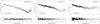 |
Fig. B.1 A comparison of the 4U 1636–53 spectra obtained with XMM-Newton, Chandra TE-mode, and Chandra CC-mode in the broadband region. Observations are combined for illustrative purposes. |
All Tables
All Figures
|
Fig. 1 Location map of the X-ray binaries of the present sample. The left panel shows the sources plotted on a full-sky map in galactic coordinates relative to the galactic center. Red points: Chandra sources. Blue points: XMM-Newton sources. The right panel shows a location map of the X-ray binaries in our sample projected in the galactic plane. |
| In the text | |
|
Fig. 2 ISMabs column densities for Chandra observations as a function of the number of counts. Black points correspond to Chandra TE-mode spectra and blue points to Chandra CC-mode spectra. |
| In the text | |
|
Fig. 3 ISMabs column densities values for each source. Gray boxes correspond to a 2σ region around the average value. |
| In the text | |
|
Fig. 4 Comparison of hydrogen column densities from different 21 cm surveys with the present ISMabs results. Black data points corresponds to the ISMabs/21 cm ratio using the Dickey & Lockman (1990) measurements. The solid color lines are linear fits to the ISMabs/21 cm values relative to the various determinations from the 21 cm surveys: Dickey & Lockman (1990, red line), Kalberla et al. (2005, green line) and Willingale et al. (2013, blue line). |
| In the text | |
|
Fig. 5 Comparison of the oxygen, neon, and iron total column densities obtained from the ISMabs model as function of distance (left panels), latitude absolute value (middle panels), and longitude (right panels) for all the analysed sources. Longitude has been rescaled to 0°−180°. |
| In the text | |
|
Fig. 6 Comparison of the abundance ratios NO/NNe (top panel) and NFe/NNe (bottom panel) obtained from the broadband fit with ISMabs for all the analysed sources. The best fitted Nx/NNe ratio for all sources is plotted with a solid red line. Ratios obtained from Grevesse & Sauval (1998), Asplund et al. (2009), Lodders et al. (2009) and Juett et al. (2004) are respectively shown with green, blue, orange and magenta dashed lines. |
| In the text | |
|
Fig. 7 Comparison of the ionization fractions O ii/O i, O iii/O i, Ne ii/Ne i, and Ne iii/Ne i obtained with the ISMabs model as function of distance (left panels), the latitude absolute value (middle panels), and longitude (right panels) for all the analysed sources. Longitude has been rescaled to 0°−180°. |
| In the text | |
|
Fig. 8 GS 1826–238 XMM-Newton spectra in the oxygen K-edge region. Observations were combined for illustrative purposes. |
| In the text | |
|
Fig. A.1 ISMabs best broadband fits for the analysed sources where observations are combined for illustrative purposes. In the case of Chandra the read mode (CC-mode or TE-mode) is indicated. |
| In the text | |
|
Fig. A.2 ISMabs best broadband fits for the analysed sources where observations are combined for illustrative purposes. In the case of Chandra the read mode (CC-mode or TE-mode) is indicated. |
| In the text | |
|
Fig. A.3 ISMabs best broadband fits for Sco X-1. Observations were combined for illustrative purposes. |
| In the text | |
|
Fig. B.1 A comparison of the 4U 1636–53 spectra obtained with XMM-Newton, Chandra TE-mode, and Chandra CC-mode in the broadband region. Observations are combined for illustrative purposes. |
| In the text | |
Current usage metrics show cumulative count of Article Views (full-text article views including HTML views, PDF and ePub downloads, according to the available data) and Abstracts Views on Vision4Press platform.
Data correspond to usage on the plateform after 2015. The current usage metrics is available 48-96 hours after online publication and is updated daily on week days.
Initial download of the metrics may take a while.