| Issue |
A&A
Volume 588, April 2016
|
|
|---|---|---|
| Article Number | A52 | |
| Number of page(s) | 11 | |
| Section | Atomic, molecular, and nuclear data | |
| DOI | https://doi.org/10.1051/0004-6361/201527615 | |
| Published online | 17 March 2016 | |
Plasma code for astrophysical charge exchange emission at X-ray wavelengths
1
SRON Netherlands Institute for Space Research,
Sorbonnelaan 2, 3584 CA
Utrecht, The
Netherlands
e-mail:
This email address is being protected from spambots. You need JavaScript enabled to view it.
2
Leiden Observatory, Leiden University,
PO Box 9513, 2300 RA
Leiden, The
Netherlands
3
Astronomical Institute “Anton Pannekoek”, University of
Amsterdam, Science Park
904, 1098 XH
Amsterdam, The
Netherlands
Received: 22 October 2015
Accepted: 22 January 2016
Abstract
Charge exchange X-ray emission provides unique insight into the interactions between cold and hot astrophysical plasmas. Besides its own profound science, this emission is also technically crucial to all observations in the X-ray band, since charge exchange with the solar wind often contributes a significant foreground component that contaminates the signal of interest. By approximating the cross sections resolved to n and l atomic subshells and carrying out complete radiative cascade calculation, we have created a new spectral code to evaluate the charge exchange emission in the X-ray band. Compared to collisional thermal emission, charge exchange radiation exhibits enhanced lines from large-n shells to the ground, as well as large forbidden-to-resonance ratios of triplet transitions. Our new model successfully reproduces an observed high-quality spectrum of comet C/2000 WM1 (LINEAR), which emits purely by charge exchange between solar wind ions and cometary neutrals. It demonstrates that a proper charge exchange model will allow us to probe the ion properties remotely, including charge state, dynamics, and composition, at the interface between the cold and hot plasmas.
Key words: atomic data / atomic processes / comets: individual: C/2000 WM1 (LINEAR)
© ESO, 2016
1. Introduction
Charge exchange (CX hereafter) occurs when an atom collides with a multicharged ion. It produces X-ray line emission if the ion charge is reasonably strong. The first discovery of CX X-ray emission in astronomical objects was made by observing the comet C/Hyakutake 1996 B2 with the ROSAT telescope (Lisse et al. 1996; Cravens 1997). This opened up a new research field to X-ray astronomers, and the related study soon expanded to various types of celestial objects. The CX process can partly explain the soft X-ray (<2 keV) spectrum of the polar component in Jupiter and other planets in the solar system (e.g., Bhardwaj 2006; Branduardi-Raymont et al. 2007). As suggested in many papers, such as Cox (1998), Cravens (2000), Snowden et al. (2004), and Fujimoto et al. (2007), the geocoronal and heliospheric area is also glowing in soft X-rays by the CX between solar wind ions and interstellar neutral atoms. CX is also a potential mechanism for X-ray emission from the North Polar Spur region (Lallement 2009), stellar winds of supergiants (Pollock 2007), shock rims of supernova remnants (Katsuda et al. 2011; Cumbee et al. 2014), starburst galaxies (Tsuru et al. 2007; Liu et al. 2011), and even clusters of galaxies (Walker et al. 2015).
The astronomical discoveries of CX emission have also stimulated theoretical and laboratory studies of this process. Recent atomic calculations based on the quantum mechanical close coupling method (e.g., Wu et al. 2011; Nolte et al. 2012) have so far provided the most reliable estimate of the cross section for single electron capture in the low-velocity regime. Laboratory investigations broadened the species of neutral reactants from the hydrogen atom to various molecules (e.g., CO, H2O), to match the real conditions better, especially for comets (Bodewits et al. 2006; Wargelin et al. 2008).
To link the atomic and astrophysical work on the CX process, we present here a new spectral model that features the most recent atomic data and a complete radiative transition calculation. Another model for CX has been introduced by Smith et al. (2014), which is more focused on the transition calculation than on the actual reaction cross section. In Sect. 2, we describe the physical assumption of our model. In Sect. 3, we show in detail how the CX line emission is calculated from basic atomic data. In Sect. 4, we demonstrate our model by applying it to real data.
Collected charge exchange data.
2. Assumptions
Our CX emission model is calculated based on three key assumptions. First, the charge transfer rates are obtained based on single electron capture in ion-neutral collision. Although multi-electron neutral targets might be important for some environments (e.g., comets) where the channels of multi-electron capture do exist (e.g., Bodewits et al. 2006), the data available on such reactions are much less complete than those for single electron capture. As shown in the experimental results of, for example, Greenwood et al. (2001), single capture can provide a first-order approximation to multi-electron reactions. Secondly, as a related issue, we assume that the CX with atomic hydrogen is a reasonable representative of the real case, in terms of the cross section dependences on ion velocity and captured electron state (see details in Sect. 3). To correct for the helium atom, we approximate the helium cross section using the scaling rule of Janev & Gallagher (1984),  (1)where NHe and NH are the numbers of valence electrons, and IHe and IH are the ionization potentials. For plasmas with cosmological abundances (10% and 90% in number for helium and hydrogen, respectively), the combined CX cross section can be derived from the pure hydrogen value by σ = 0.96σH.
As the third assumption, the radiative processes related to free electrons, e.g., collisional excitation and radiative/dielectron recombination, are ignored in the modeling. It will prevent the CX-induced transitions, which usually involves large-n shells (Sect. 3.2), from being overpowered in emission by the collisional excitation dominating the small-n shells. This assumption can be validated because the ionic CX has much larger cross section than the electronic processes at X-ray energies.
3. Method
To calculate CX line emission, we first determine the ion state population after electron capture, and then solve the possible radiative cascading pathways to the ground state. The first step can be further divided into three components, i.e., the total capture cross sections, and the cross sections into each n- and l-resolved level.
The main challenge is that the current atomic data for n- and l-resolved cross sections are far from complete. It is therefore necessary to investigate the available data for intrinsic scaling relations among n- and l-resolved parameters, as described in Sects. 3.2 and 3.3, respectively. In practice, we collected all available cross sections from the literature and applied the derived scaling relations when the actual data are absent.
3.1. Total cross sections
It is commonly believed that CX has a very large cross section compared to electronic processes, typically of about 10-15−10-14 cm-2. To obtain the cross section as a function of collision velocity v, we compiled the results reported in previous theoretical calculations (Ryufuku 1982; Shipsey et al. 1983; Fritsch & Lin et al. 1984; Phaneuf et al. 1987; Janev et al. 1988, 1993; Olson & Schultz 1989; Belkić 1991; Harel et al. 1998; Whyte et al. 1998; Perez et al. 2001; Errea et al. 2004; Schultz et al. 2010; Wu et al. 2011; Nolte et al. 2012) and experimental measurements (Fite et al. 1962; Olson et al. 1977; Meyer et al. 1979, 1985; Crandall et al. 1979). A complete list of the data sources is shown in Table 1. For the theoretical calculations, we employed a practical criterion reported in Janev et al. (1993), which depends on the calculation method, to assess the energy range of validity.
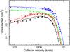 |
Fig. 1 Total cross sections, as functions of collision velocity, for B5 + (black), O8 + (red), Ne10 + (green), and Ar18 + (blue) interacting with a hydrogen atom. The data points are actual values from previous calculations, and solid lines are the scaling law described in Sect. 3.1. |
As shown in Wargelin et al. (2008), for example, the average cross sections usually exhibit a linear dependence on ion charge q. Such a feature is also seen in Fig. 1. In addition, due to the non-resonant effect (e.g., Janev & Winter 1985), the cross sections for small-q reactions, e.g., B5 + with the H atom, exhibit a maximum at certain v ≤ v0 (where v0 is the orbital velocity of bound electrons), and exponential decrease toward low energy. For large-q ions, such as Ne10 + and Ar18 +, this effect diminishes as the number of channels for resonant reactions becomes large. In the high energy regime (v>v0), both small-q and large-q reactions fall off as charge transfer into discrete levels become strongly coupled with the continuum, and the ionization process starts to dominate. To combine the q- and v-dependence, we use a scaling law refined from Janev & Smith (1993), 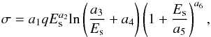 (2)where Es = E/q0.43 is a scaled version of the collision energy E given in eV/amu, and a1 to a6 are q-dependent fitting parameters. The average best-fit values for a1 to a6 are (4.6, 1.0, 0.2, 1.0, 83., −8.9) and (0.3, 0.1, 1., 10., 158., −9.9), for 3 <q< 10 and q ≥ 10, respectively. As shown in Fig. 1, the scaling relation in general reproduces the cross sections of all ions well. Some residuals are seen at v ≤ 500 km s-1, where the data oscillate around the fitting curve for small-q species. This is probably caused by the discrete nature of product ion energy levels (e.g., Ryufuku 1980). In practice, since the actual data for such small-q species are usually available in the literature, the bias on the scaling relation can barely affect our model. Equation (2) is then used to calculate cross sections for ions that are still missing in previous publications.
3.2. n-shell populations
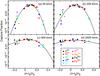 |
Fig. 2 Fractions of single electron capture into n shell, at v = 50 km s-1a); 200 km s-1b); 900 km s-1c); and 2400 km s-1d); as a function of (n − np) /np. Different sets of data points represent different projectile ions, as indicated in d); and the solid lines are the polynomial fitting to the data. |
The CX probability reaches its maximum when the two energy states, before and after the transition, are closest to each other. For low-speed collisions (v ≪ v0), the potential energy dominates the interaction, and the principle quantum number np of the most populated energy level can be written by 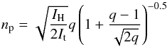 (3)(Janev & Winter 1985), where IH and It are the ionization potentials of H and the target atom, respectively. This means that the peak level is determined by the combined potential of the projectile ion and target atom. For most ions, np is much larger than unity. In the high-speed regime (v ~ v0), the collision dynamics become more important for the capture process, and the peak population level is gradually smeared out among several adjacent shells.
We compiled the velocity-dependent, n-resolved cross sections for reactions involving Be, B, C, N, O, Ne, and Fe ions from theoretical calculations (Ryufuku 1982; Shipsey et al. 1983; Fritsch & Lin et al. 1984; Belkić et al. 1992; Janev et al. 1993; Toshima & Tawara 1995; Harel et al. 1998; Rakovi et al. 2001; Errea et al. 2004; Nolte et al. 2012; Wu et al. 2011, 2012; Mullen et al. 2015). As shown in Fig. 2, the capture cross sections are normalized to the total value of each ion and plotted against (n − np) /np. This puts them on a roughly similar n-distribution function, which reconfirms the result in Janev & Winter (1985). The velocity dependence of the n-populations also agrees with the consensus described above. As seen in Fig. 2, for each velocity, we fit the n-distribution by a phenomenological third-degree polynomial curve, which reproduces the data. Some minor deviations, typically a few percent of the total cross section, are seen for low-capture shells. The same fitting was done for ten other velocity points to fully cover the range of 50 ≤ v ≤ 5000 km s-1. Details of the fitting procedure can be found in Appendix A. As a first-order approximation, we assumed that all the CX processes with hydrogen-atom targets follow the same profile in the (n − np) /np versus σ space and have a similar velocity dependence. In this way, the n-resolved populations were calculated for all the rest ions. When applying the n-distribution to astrophysical plasmas contaminated by helium, the actual peak n would be slightly lower than the calculated value, since the helium target has a larger ionization potential than atomic hydrogen. Assuming the cosmic abundances, this would lead to an uncertainty of ≤10% for the obtained n-resolved cross sections.
3.3. l-subshell populations
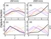 |
Fig. 3 Averaged fractions of l-dependent capture for N7 + and O7 +, plotted as a function of l. Black solid lines are the data from theoretical calculations, and the red, blue, magenta, and orange dashed lines are empirical functions shown in Eqs. (4)–(6), (8), respectively. Panels a) and b) are the capture for n = 4 at v = 200 km s-1 and 2000 km s-1, respectively, and c) and d) are those for n = 5. |
Besides the n-dependent capture, it is known that the CX process also exhibits strong selective properties with respect to the final electron orbit angular momentum l. As discussed in Janev & Winter (1985) and Suraud et al. (1991), for example, the l-selectivity is very sensitive to the collision velocity and is often governed by high-order processes in the transition (e.g., rotational mixing). Typically, the l distribution is approximated as a function of n, l, and q in at least five forms shown as follows: ![Mathematical equation: \begin{equation} W^{\rm l1}_{n}(l) = (2l + 1) \frac{[(n-1)!]^{2}} {(n+l)!(n-l-1)!} \:\:\:\:\:\:\:\:\:\:\:\:\:\:\:\:\: \bf(low \: energy \: I), \end{equation}](/articles/aa/full_html/2016/04/aa27615-15/aa27615-15-eq88.png) (4)
(4) (5)
(5)![Mathematical equation: \begin{equation} W^{\rm se}_{n}(l) = \left(\frac{2l+1}{q}\right) {\rm exp}\left[-\frac{l(l+1)}{q}\right] \:\:\:\:\:\:\:\:\:\:\:\:\:\:\:\:\:\:\:\: \bf(separable), \end{equation}](/articles/aa/full_html/2016/04/aa27615-15/aa27615-15-eq90.png) (6)
(6) (7)
(7) (8)In the low velocity regime (v ≪ v0), generally the transferred electron does not carry sufficient angular momentum to populate large-l subshells. These electrons form a peak at l = 1 or 2 (e.g., Abramov et al. 1978), which can be roughly described by functions Wl1, Wl2, and/or Wse. As the collision velocity increases, the l peak is gradually smeared out by rotational mixing of the coupling Stark states, and the subshells are populated according to the statistical weight Wst.
It is clear that none of the five functions alone can describe the l-populations for all velocities. Previous work further suggested that the choice of weighting function also depends on the principle quantum number n; the l-distributions of n ≤ np subshells are often found to be different from those with n>np (e.g., Janev & Winter 1985). To elucidate the v- and n-dependence, we plot in Figs. 3a and c the averaged l-distributions at v = 200 km s-1 for N7 + and O7 + ions, based on data from theoretical calculations (Belkić et al. 1992; Toshima & Tawara 1995; Rakovi et al. 2001). The two dominant shells with n = 4 and 5 are used to represent the n ≤ np and n>np groups, respectively. This is valid since the rest shells contribute less than 0.1% of the total rate at v = 200 km s-1. The N7 + and O7 + ions exhibit a large capture fraction into l = 1 for n = 5, while for n = 4, subshells with l = 2 and 3 are equally or even more populated than l = 1. By comparing data with the five weighting functions, we found that the l-populations of the two ions are best approximated by the Wl2 function at n = 5, while the n = 4 shells resemble the Wse function more. As shown in Figs. 3b and d, the same calculation was done at v = 2000 km s-1, where the two distributions become roughly consistent and match the statistical weight Wst best. By incorporating the data of other available ions, we determined the preferred weighting function, dependent on v and n, and applied it to the rest ions (see Appendix B for details).
3.4. Spectral model
The CX emission line is produced when the captured electron relaxes to the valence shell of the ground state of the product ion. To perform the complete cascade calculation, we obtained the energies and transition probabilities for all the atomic levels up to n = 16, which exceeds the maximum capture state for all ions used in the code (e.g., maximum capture n = 12 and 13 for Fe25+ + H collision). The FAC code for theoretical atomic calculations (Gu 2008) was used as a baseline tool, and the energies were calibrated to those derived with another atomic structure code (Cowan 1981), as well as the experimental measurements at the National Institute of Standards and Technology1. The line spectrum was then calculated from the cascade network given the source term of the CX rates. More features of the new CX model are described in Appendix C.
As described in Sect. 3.2, the CX process can populate the large-n shells, so line emission from such shells is strongly enhanced compared to collisional thermal radiations. For instance, the O viii Lyδ line at 14.8 Å is stronger than the Lyγ line at 15.2 Å. Similar conditions can be found in many other transitions: e.g., the O vii Heδ line at 17.4 Å, the N vii Lyδ line at 19.4 Å, and C vi Lyδ line at 26.4 Å. The derived CX spectrum also features a large G ratio, the forbidden plus intercombination lines to resonance line ratio, since the collisional excitation process becomes negligible in CX plasmas (Sect. 2).
3.5. Bias from systematic weight
As reported recently by Nolte et al. (2012), the singlet-to-triplet ratio of the C4 + ion, produced from a low-velocity C5 ++ H reaction, covers a broad range of 0.01−100 for different n, l, and v. The apparent bias from the commonly adopted statistical value 3 is probably caused by electron-electron interaction during the capture. A similar effect was also reported in other papers (e.g., Wu et al. 2011 for N6 ++ H reaction), indicating that it could be a common property. Although the current data are still too sparse to fully implement the S-dependence, it is vital to estimate the induced biases on emission line ratios. As shown in Fig. 4, we compare the G ratio calculated based on the data from Nolte et al. (2012) with that assuming statistical weight for the C5 + + H reaction. The largest bias is seen at v ~ 500 km s-1, where the statistical weight is underestimated by about 30%. The two ratios become roughly consistent at low and high velocity ends. The figure suggests that the current code can cover the actual G ratio range, although the derived velocity would have a systematic error up to 200−300 km s-1.
4. Real data fitting
To verify the CX model, we fit it to the real data of comet C/2000 WM1 (LINEAR) observed by the XMM-Newton Reflection Grating Spectrometer (RGS), which has a high spectral resolution ~0.07 Å in soft X-rays (5−38Å). Comets are the favorite target for our purpose, since they emit bright X-rays that are produced exclusively by the CX between the highly charged heavy ions in the solar wind and cometary atmosphere (Dennerl 2010). As a caveat, the current model is based on an atomic hydrogen target, while the cometary neutrals are mainly moleculars, such as H2O and CO. As reported in Bodewits et al. (2007) and Mullen et al. (2015), the cross sections of moleculars can be roughly approximated by that of H at intermediate and high velocities, while at low velocity (v ≲ 100 km s-1), they become different by orders of magnitude. The cometary CX model with molecular targets will be reported in a subsequent paper (Mullen et al., in prep.).
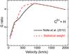 |
Fig. 4 G ratio of C v Heα triplets, calculated based on the triplet-to-singlet ratios reported in Nolte et al. (2012, black) and the value given by statistical weight (red). |
4.1. Observation
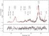 |
Fig. 5 CX fitting (red) to the RGS spectrum (black) of comet C/2000 WM1 (LINEAR). |
Comet C/2000 WM1 was observed by XMM-Newton on December 2001 for a continuous exposure of about 62 ks. The RGS event files were created by using SAS 14.0 and the most recent calibration files. To remove events outside the field of view along the cross-dispersion direction (5′), we used only the 18 ks exposure when the comet was close to the center point of the detector. The background component was approximated by the model background spectrum calculated by SAS tool rgsproc. To correct the spectral broadening due to spatial extent of the cometary X-ray halo, we used a 7−30Å image that was observed at the same period with the MOS1 detector of the European Photon Imaging Cameras (EPIC) onboard XMM-Newton. The final RGS data has more than 18 000 counts recorded with high spectral resolution, making it the best X-ray data so far for the cometary CX study.
4.2. Results
Our study focuses on the 22−38Å (0.33−0.56 keV) band of the RGS spectrum. In the fits, we assume that all the solar wind ions have a same ionization temperature and collided with the comet atmosphere at a constant velocity during the exposure. The temperature and velocity are allowed to vary freely. We can also measure the C, N, O, Mg, and Si abundances of the wind, but other elements are not visible in the RGS energy band. Following the recipe of von Steiger et al. (2000), the solar abundances are set to the photospheric values from Grevesse & Sauval (1998). The CX emissivity, which is determined by combining the ion and neutral densities, was also set free, although it would degenerate with the metal abundances to some extent. As shown in Fig. 5, the RGS spectrum can be fit reasonably well by one CX component, characterized by an ionization temperature of 0.14 ± 0.01 keV and a collision velocity of  km s-1. The fitting C statistic is 401 for a degree of freedom of 288. The collision velocity is measured primarily by the strong C vi lines from different n shells, including the Lyα line at 33.7 Å, the Lyβ line at 28.5 Å, the Lyγ line at 27.0 Å, and the Lyδ line at 26.4 Å. The N vii and O vii series also help in the velocity measurement. The smaller lower velocity error compared to the upper one is probably because the line ratios become more sensitive to the velocities at lower collision energies. The best-fit abundance ratios relative to O (C/O, N/O, Mg/O, and Si/O) are measured to be 1.9 ± 0.3, 1.6 ± 0.6, 5 ± 4, and 3 ± 2, respectively. These values are roughly consistent with the average solar wind abundances reported in von Steiger et al. (2000).
The derived CX component appears to resemble the slow-type solar wind. It is well known that the slow wind is launched with a typical ionization state of 0.12−0.14 keV, which is quite different from that of a fast wind (0.07 keV, Feldman et al. 2005). The ionization temperature remains nearly the same in the wind propagation, since the ionization/recombination timescales are often much longer than the travel time. On the other hand, according to the records of Advanced Composition Explorer (ACE), the solar wind ion speed at the Earth Lagrangian point L1 is in the range of 250−350 km s-1, in the period of the C/2000 WM1 observation by XMM-Newton. Since the heliocentric distance of the comet was nearly 1 AU, the ion speed at its environment should be close to the ACE record (Neugebauer et al. 2000). Consider that the comet had a velocity of ~50 km s-1 relative to the Sun, the best-fit collision velocity measured with our CX model appears to be slightly lower than the wind speed in the comet restframe. This agrees with the picture presented in Bodewits et al. (2007), among others, in which the solar wind is somewhat decelerated in the comet bow shock region.
5. Summary
We developed a new plasma code to calculate charge exchange emission in X-ray band. To overcome the incompleteness in atomic data of cross sections, we derived scaling laws to approximate the n- and l-distributions for various collision velocities in the range of 50−5000 km s-1. The radiative cascading calculation shows characteristic charge exchange emission features, including both high-shell transition lines and large G ratios of triplets. Our CX model successfully reproduces an observed high resolution X-ray spectrum from comet C/2000 WM1 with reasonable ionization temperature and collision velocity of the solar wind ions.
Acknowledgments
SRON is supported financially by NWO, the Netherlands Organization for Scientific Research.
References
- Abramov, V. A., Baryshnikov, F. F., & Lisitsa, V. S. 1978, Sov. J. Exp. Theor. Phys. Lett., 27, 464 [NASA ADS] [Google Scholar]
- Belkić, D. 1991, Phys. Scr, 43, 561 [Google Scholar]
- Belkić, D., Gayet, R., & Salin, A. 1992, Atom. Data Nucl. Data Tables, 51, 59 [Google Scholar]
- Bhardwaj, A. 2006, Advances in Geosciences, Planetary Science (PS) (World Scientific Co, Pte. Ltd.), 215 [Google Scholar]
- Branduardi-Raymont, G., Bhardwaj, A., Elsner, R. F., et al. 2007, A&A, 463, 761 [NASA ADS] [CrossRef] [EDP Sciences] [Google Scholar]
- Bodewits, D., Hoekstra, R., Seredyuk, B., et al. 2006, ApJ, 642, 593 [NASA ADS] [CrossRef] [Google Scholar]
- Bodewits, D., Christian, D. J., Torney, M., et al. 2007, A&A, 469, 1183 [NASA ADS] [CrossRef] [EDP Sciences] [Google Scholar]
- Cowan, R. D. 1981, Los Alamos Series in Basic and Applied Sciences (Berkeley: University of California Press) [Google Scholar]
- Cox, D. P. 1998, Lect. Notes Phys., 506, 121 [NASA ADS] [CrossRef] [Google Scholar]
- Crandall, D. H., Phaneuf, R. A., & Meyer, F. W. 1979, Phys. Rev. A, 19, 504 [NASA ADS] [CrossRef] [Google Scholar]
- Cravens, T. E. 1997, Geophys. Res. Lett., 24, 105 [NASA ADS] [CrossRef] [Google Scholar]
- Cravens, T. E. 2000, ApJ, 532, L153 [NASA ADS] [CrossRef] [PubMed] [Google Scholar]
- Cumbee, R. S., Henley, D. B., Stancil, P. C., et al. 2014, ApJ, 787, L31 [NASA ADS] [CrossRef] [Google Scholar]
- Dennerl, K. 2010, Space Sci. Rev., 157, 57 [NASA ADS] [CrossRef] [Google Scholar]
- Errea, L. F., Illescas, C., Méndez, L., et al. 2004, J. Phys. B At. Mol. Phys., 37, 4323 [Google Scholar]
- Feldman, U., Landi, E., & Schwadron, N. A. 2005, J. Geophys. Res. (Space Phys.), 110, A07109 [Google Scholar]
- Fite, W. L., Smith, A. C. H., & Stebbings, R. F. 1962, Roy. Soc. London Proc. Ser. A, 268, 527 [Google Scholar]
- Fritsch, W., & Lin, C. D. 1984, Phys. Rev. A, 29, 3039 [NASA ADS] [CrossRef] [Google Scholar]
- Fujimoto, R., Mitsuda, K., Mccammon, D., et al. 2007, PASJ, 59, 133 [NASA ADS] [Google Scholar]
- Greenwood, J. B., Williams, I. D., Smith, S. J., & Chutjian, A. 2001, Phys. Rev. A, 63, 062707 [NASA ADS] [CrossRef] [Google Scholar]
- Grevesse, N., & Sauval, A. J. 1998, Space Sci. Rev., 85, 161 [NASA ADS] [CrossRef] [Google Scholar]
- Gu, M. F. 2008, Can. J. Phys., 86, 675 [NASA ADS] [CrossRef] [Google Scholar]
- Harel, C., Jouin, H., & Pons, B. 1998, Atom. Data Nucl. Data Tables, 68, 279 [Google Scholar]
- Janev, R. K., & Gallagher, J. W. 1984, J. Phys. Chem. Ref. Data, 13, 1199 [NASA ADS] [CrossRef] [Google Scholar]
- Janev, R. K., & Smith, J. J. 1993, Atomic and Plasma-Material Interaction Data for Fusion (Supplement to the journal Nuclear Fusion), 4, 1 [Google Scholar]
- Janev, R. K., & Winter, H. 1985, Phys. Rep., 117, 265 [NASA ADS] [CrossRef] [Google Scholar]
- Janev, R. K., Phaneuf, R. A., & Hunter, H. T. 1988, Atom. Data Nucl. Data Tables, 40, 249 [NASA ADS] [CrossRef] [Google Scholar]
- Janev, R. K., Phaneuf, R. A., Tawara, H., & Shirai, T. 1993, Atom. Data Nucl. Data Tables, 55, 201 [Google Scholar]
- Kaastra, J. S., Mewe, R., & Nieuwenhuijzen, H. 1996, in 11th Colloq. on UV and X-ray Spectroscopy of Astrophysical and Laboratory Plasmas, 411 [Google Scholar]
- Katsuda, S., Tsunemi, H., Mori, K., et al. 2011, ApJ, 730, 24 [NASA ADS] [CrossRef] [Google Scholar]
- Lallement, R. 2009, Space Sci. Rev., 143, 427 [NASA ADS] [CrossRef] [Google Scholar]
- Lisse, C. M., Dennerl, K., Englhauser, J., et al. 1996, Science, 274, 205 [NASA ADS] [CrossRef] [EDP Sciences] [Google Scholar]
- Liu, J., Mao, S., & Wang, Q. D. 2011, MNRAS, 415, L64 [NASA ADS] [CrossRef] [Google Scholar]
- Meyer, F. W., Phaneuf, R. A., Kim, H. J., Hvelplund, P., & Stelson, P. H. 1979, Phys. Rev. A, 19, 515 [NASA ADS] [CrossRef] [Google Scholar]
- Meyer, F. W., Howald, A. M., Havener, C. C., & Phaneuf, R. A. 1985, Phys. Rev. A, 32, 3310 [NASA ADS] [CrossRef] [PubMed] [Google Scholar]
- Mullen, P. D., Cumbee, R., Lyons, D., Stancil, P. C., & B. J. Wargelin 2015, AAS Meet. Abst., 225, #407.02 [Google Scholar]
- Neugebauer, M., Cravens, T. E., Lisse, C. M., et al. 2000, J. Geophys. Res., 105, 20949 [NASA ADS] [CrossRef] [Google Scholar]
- Nolte, J. L., Stancil, P. C., Liebermann, H. P., et al. 2012, J. Phys. B At. Mol. Phys., 45, 245202 [NASA ADS] [CrossRef] [Google Scholar]
- Olson, R. E., & Schultz, D. R. 1989, Phys. Scr. T, 28, 71 [NASA ADS] [CrossRef] [Google Scholar]
- Olson, R. E., Salop, A., Phaneuf, R. A., & Meyer, F. W. 1977, Phys. Rev. A, 16, 1867 [NASA ADS] [CrossRef] [Google Scholar]
- Perez, J. A., Olson, R. E., & Beiersdorfer, P. 2001, J. Phys. B At. Mol. Phys., 34, 3063 [NASA ADS] [CrossRef] [Google Scholar]
- Phaneuf, R. A., Janev, R. K., & Pindzola, M. S. 1987, Collisions of carbon and oxygen ions with electrons, H, H2 and He (Springfield, Va.: Controlled Fusion Atomic Data Center) Available from National Technical Information Service, Atomic data for fusion, 0888-8345; vol. 5. Controlled Fusion Atomic Data Center (Oak Ridge National Laboratory) [Google Scholar]
- Pollock, A. M. T. 2007, A&A, 463, 1111 [NASA ADS] [CrossRef] [EDP Sciences] [Google Scholar]
- Raković, M. J., Wang, J., Schultz, D. R., & Stancil, P. C. 2001, AGU Spring Meeting Abstracts, 41 [Google Scholar]
- Ryufuku, H. 1982, Phys. Rev. A, 25, 720 [NASA ADS] [CrossRef] [Google Scholar]
- Ryufuku, H., Sasaki, K., & Watanabe, T. 1980, Phys. Rev. A, 21, 745 [NASA ADS] [CrossRef] [Google Scholar]
- Schultz, D. R., Lee, T.-G., & Loch, S. D. 2010, J. Phys. B At. Mol. Phys., 43, 144002 [NASA ADS] [CrossRef] [Google Scholar]
- Shipsey, E. J., Green, T. A., & Browne, J. C. 1983, Phys. Rev. A, 27, 821 [Google Scholar]
- Smith, R. K., Foster, A. R., Edgar, R. J., & Brickhouse, N. S. 2014, ApJ, 787, 77 [NASA ADS] [CrossRef] [Google Scholar]
- Snowden, S. L., Collier, M. R., & Kuntz, K. D. 2004, ApJ, 610, 1182 [NASA ADS] [CrossRef] [Google Scholar]
- Suraud, M. G., Hoekstra, R., de Heer, F. J., Bonnet, J. J., & Morgenstern, R. 1991, J. Phys. B At. Mol. Phys., 24, 2543 [Google Scholar]
- Toshima, N., & Tawara, H. 1995, NIFS-DATA-026, www.nifs.ac.jp/report/nifs-data026.html [Google Scholar]
- Tsuru, T. G., Ozawa, M., Hyodo, Y., et al. 2007, PASJ, 59, 269 [NASA ADS] [Google Scholar]
- von Steiger, R., Schwadron, N. A., Fisk, L. A., et al. 2000, J. Geophys. Res., 105, 27217 [NASA ADS] [CrossRef] [Google Scholar]
- Walker, S. A., Kosec, P., Fabian, A. C., & Sanders, J. S. 2015, MNRAS, 453, 2480 [NASA ADS] [Google Scholar]
- Wargelin, B. J., Beiersdorfer, P., & Brown, G. V. 2008, Can. J. Phys., 86, 151 [NASA ADS] [CrossRef] [Google Scholar]
- Whyte, D. G., Isler, R. C., Wade, M. R., et al. 1998, Phys. Plasmas, 5, 3694 [NASA ADS] [CrossRef] [Google Scholar]
- Wu, Y., Stancil, P. C., Liebermann, H. P., et al. 2011, Phys. Rev. A, 84, 022711 [NASA ADS] [CrossRef] [Google Scholar]
- Wu, Y., Stancil, P. C., Schultz, D. R., et al. 2012, J. Phys. B At. Mol. Phys., 45, 235201 [NASA ADS] [CrossRef] [Google Scholar]
Appendix A: Fitting the n distributions
It has long been known that the CX cross section often distributes continuously as a function of n with a maximum near np, when the ion charge q is sufficiently large (see Janev & Winter 1985 for a review). To quantify the n distribution, we compiled the velocity- and n- dependent cross sections found in literature in Sect. 3.2 and fit them with a phenomenological third-degree polynomial curve, ![Mathematical equation: \appendix \setcounter{section}{1} \begin{equation} \begin{aligned} \lg \sigma_{\rm norm}(n) = {} & c_{1}(v) + c_{2}(v) n_{\rm norm}(n,q) + c_{3}(v) n_{\rm norm}^{2}(n,q) \\[2mm] & + c_{4}(v) n_{\rm norm}^{3}(n,q), \end{aligned} \end{equation}](/articles/aa/full_html/2016/04/aa27615-15/aa27615-15-eq140.png) (A.1)where σnorm(n) is the capture fraction into n, c1(v) to c4(v) are four velocity-dependent fitting parameters, and nnorm(n,q) = (n − np) /np. The best-fit parameters are shown in Table A.1.
(A.1)where σnorm(n) is the capture fraction into n, c1(v) to c4(v) are four velocity-dependent fitting parameters, and nnorm(n,q) = (n − np) /np. The best-fit parameters are shown in Table A.1.
n-distribution fitting parameters
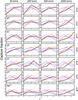 |
Fig. A.1 Averaged fractions of l-dependent capture for C5 +, N6 +, N7 +, O6 +, O7 +, O8 +, and Ne10 +, plotted as a function of l. For each ion, the dominant n-shell in n ≤ np is shown. The color and line styles are the same as in Fig. 3. |
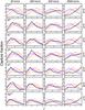 |
Fig. A.2 Averaged fractions of l-dependent capture for C5 +, N6 +, N7 +, O6 +, O7 +, O8 +, and Ne10 +, plotted as a function of l. For each ion, the dominant n-shell in n>np is shown. The color and line styles are the same as in Fig. 3. |
Appendix B: Preferred l-distributions
Here we describe in detail a velocity-dependent scheme to approximate the l-selectivity. As shown in Table 1, the l-resolved cross section data, derived from theoretical calculation, are available for reactions with the seven ions, i.e., C5 +, N6 +, N7 +, O6 +, O7 +, O8 +, and Ne10 +. For other ions, the five canonical weighting functions, as shown in Eqs. (4)–(8), were utilized as follows.
For each velocity, we determined the preferred weighting function by comparing them to the available data. As described in Sect. 3.3, the preferred function must be chosen separately for shells with principle quantum number n ≤ np and those with n>np. Here we only study the most dominant shell in each group (Figs. A.1 and A.2). For n ≤ np, the Wse function (Eq. (6)) is recommended at low velocities, i.e., v = 50 and 200 km s-1, while the statistical weight Wst becomes more popular in the intermediate- and high- velocity regimes (v = 500 and 2000 km s-1). As shown in Fig. A.1, this scheme can be applied approximately to most reactions, except for a few outliers, such as C5 + and O8 + at v = 50 km s-1, O6 + at v = 200 km s-1, and N7 + at v = 500 km s-1. As for n>np, the l-distribution is represented best by WL2 at v = 50 and 200 km s-1, Wse at v = 500 km s-1, and Wst at v = 2000 km s-1, albeit with a few exceptions such as C5 + and Ne10 + at v = 500 km s-1.
To define the l-preference continuous in the velocity space, we further analyzed the data with a finer velocity grid of 20 points. It is found that the l-distributions for n ≤ np shells mostly switch at v = 500 km s-1 from a Wse form to a Wst form, while the n>np shells are likely to evolve from Wl2 to Wse at v = 300 km s-1, and from Wse to Wst at v = 500 km s-1.
Appendix C: More features of the SPEX-CX model
Our plasma code for CX emission is included as an independent model in the SPEX package (Kaastra et al. 1996)2. The model first calculates the fraction of each ion at a ionization temperature Ti and element abundance A, then evaluates the CX spectrum for a collision velocity v and emission measure norm. The rate coefficients obtained in Sect. 3 are fully utilized in the model, and the actual data are tabulated in the form of FITS files3 in the SPEX database. They will be updated with more recent published results once these become available.
The CX model contains three additional parameters for different physical conditions. First, the collision velocity v can be replaced by the velocity of random thermal motion, which is characterized by ion temperature Ti. This is appropriate for some hot plasmas where thermal motion dominates. Second, besides the single collision mode, our model also allows multiple collisions between ions and neutrals. In the latter case, one ion would continuously undergo CX and produce various emission lines, until it becomes neutral. This is suited more to objects with dense neutral materials. Finally, the model provides five types of l-weighting functions (Eqs. (4)–(8)) for the CX cross section. The optimized method is described in Sect. 3.3, while the five basic functions can also be selected to fine-tune the spectrum and to test the sensitivity of data to the assumed subshell populations.
All Tables
All Figures
|
Fig. 1 Total cross sections, as functions of collision velocity, for B5 + (black), O8 + (red), Ne10 + (green), and Ar18 + (blue) interacting with a hydrogen atom. The data points are actual values from previous calculations, and solid lines are the scaling law described in Sect. 3.1. |
| In the text | |
|
Fig. 2 Fractions of single electron capture into n shell, at v = 50 km s-1a); 200 km s-1b); 900 km s-1c); and 2400 km s-1d); as a function of (n − np) /np. Different sets of data points represent different projectile ions, as indicated in d); and the solid lines are the polynomial fitting to the data. |
| In the text | |
|
Fig. 3 Averaged fractions of l-dependent capture for N7 + and O7 +, plotted as a function of l. Black solid lines are the data from theoretical calculations, and the red, blue, magenta, and orange dashed lines are empirical functions shown in Eqs. (4)–(6), (8), respectively. Panels a) and b) are the capture for n = 4 at v = 200 km s-1 and 2000 km s-1, respectively, and c) and d) are those for n = 5. |
| In the text | |
|
Fig. 4 G ratio of C v Heα triplets, calculated based on the triplet-to-singlet ratios reported in Nolte et al. (2012, black) and the value given by statistical weight (red). |
| In the text | |
|
Fig. 5 CX fitting (red) to the RGS spectrum (black) of comet C/2000 WM1 (LINEAR). |
| In the text | |
|
Fig. A.1 Averaged fractions of l-dependent capture for C5 +, N6 +, N7 +, O6 +, O7 +, O8 +, and Ne10 +, plotted as a function of l. For each ion, the dominant n-shell in n ≤ np is shown. The color and line styles are the same as in Fig. 3. |
| In the text | |
|
Fig. A.2 Averaged fractions of l-dependent capture for C5 +, N6 +, N7 +, O6 +, O7 +, O8 +, and Ne10 +, plotted as a function of l. For each ion, the dominant n-shell in n>np is shown. The color and line styles are the same as in Fig. 3. |
| In the text | |
Current usage metrics show cumulative count of Article Views (full-text article views including HTML views, PDF and ePub downloads, according to the available data) and Abstracts Views on Vision4Press platform.
Data correspond to usage on the plateform after 2015. The current usage metrics is available 48-96 hours after online publication and is updated daily on week days.
Initial download of the metrics may take a while.