| Issue |
A&A
Volume 587, March 2016
|
|
|---|---|---|
| Article Number | A126 | |
| Number of page(s) | 12 | |
| Section | Stellar structure and evolution | |
| DOI | https://doi.org/10.1051/0004-6361/201527751 | |
| Published online | 02 March 2016 | |
Weak magnetic field, solid-envelope rotation, and wave-induced N-enrichment in the SPB star ζ Cassiopeiae⋆
1
Institut d’Astrophysique et de Géophysique, Université de
Liège,
Quartier Agora, Allée du 6 août 19C,
4000
Liège,
Belgium
e-mail:
This email address is being protected from spambots. You need JavaScript enabled to view it.
2
LESIA, Observatoire de Paris, PSL Research University, CNRS,
Sorbonne Universités, UPMC Univ.
Paris 06, Univ. Paris Diderot, Sorbonne Paris Cité, 5 place Jules
Janssen, 92195
Meudon,
France
3
Institut de Recherche en Astrophysique et Planétologie, Université
de Toulouse UPS-OMP/CNRS, 14 avenue
Edouard Belin, 31400
Toulouse,
France
Received: 16 November 2015
Accepted: 14 January 2016
Abstract
Aims. The main-sequence B-type star ζ Cassiopeiae is known as a N-rich star with a magnetic field discovered with the Musicos spectropolarimeter. We model the magnetic field of the star by means of 82 new spectropolarimetric observations of higher precision to investigate the field strength, topology, and effect.
Methods. We gathered data with the Narval spectropolarimeter installed at Télescope Bernard Lyot (TBL; Pic du Midi, France) and applied the least-squares deconvolution technique to measure the circular polarisation of the light emitted from ζ Cas. We used a dipole oblique rotator model to determine the field configuration by fitting the longitudinal field measurements and by synthesizing the measured Stokes V profiles. We also made use of the Zeeman-Doppler imaging technique to map the stellar surface and to deduce the difference in rotation rate between the pole and equator.
Results. ζ Cas exhibits a polar field strength Bpol of 100−150 G, which is the weakest polar field observed so far in a massive main-sequence star. Surface differential rotation is ruled out by our observations and the field of ζ Cas is strong enough to enforce rigid internal rotation in the radiative zone according to theory. Thus, the star rotates as a solid body in the envelope.
Conclusions. We therefore exclude rotationally induced mixing as the cause of the surface N-enrichment. We discuss that the transport of chemicals from the core to the surface by internal gravity waves is the most plausible explanation for the nitrogen overabundance at the surface of ζ Cas.
Key words: stars: magnetic field / stars: individual: zeta Cas / starspots / stars: massive / stars: abundances / stars: rotation
Based on observations obtained at the Télescope Bernard Lyot (USR5026) operated by the Observatoire Midi-Pyrénées, Université de Toulouse (Paul Sabatier), Centre National de la Recherche Scientifique (CNRS) of France.
F.R.S.-FNRS Postdoctoral Researcher, Belgium.
© ESO, 2016
1. Introduction
Among main-sequence B-type stars, it is well known that the Bp stars, B-type stars showing abnormal abundances of certain chemical elements in their atmosphere, are usually found to possess strong magnetic fields of several hundred Gauss to tens of kGauss. Weak magnetic fields of the order of a few hundreds Gauss have also been detected in several B-type targets that undergo stellar pulsations, i.e. in β Cep stars and in slowly pulsating B (SPB) stars. The first detections of weak longitudinal magnetic fields (lower than 100 G) in the group of pulsating B stars have been achieved for the β Cep stars β Cephei (Henrichs et al. 2000) and V 2052 Oph (Neiner et al. 2003b). Following these discoveries, searches for magnetic fields in β Cep and SPB stars have been accomplished (e.g. Hubrig et al. 2006, 2009; Henrichs et al. 2009; Silvester et al. 2009; Alecian et al. 2011; Briquet et al. 2013; Neiner et al. 2014c; Sódor et al. 2014), definitely showing that magnetic fields are present among B-type pulsators. However, direct detections of a Zeeman signature in the Stokes V measurements have only been obtained for ~70 magnetic massive stars and they remain limited for pulsating B stars (~15 targets). Moreover, there are only a few detailed studies of the magnetic field configuration for these objects (e.g. Hubrig et al. 2011; Henrichs et al. 2012; Neiner et al. 2012a).
The B2 IV-V star ζ Cas (HD 3360) was discovered to be magnetic with the Musicos spectropolarimeter at Télescope Bernard Lyot (TBL; Pic du Midi, France) by Neiner et al. (2003a). Independent spectroscopic determinations of the fundamental parameters (Briquet & Morel 2007; Lefever et al. 2010; Nieva & Przybilla 2012) place this target in the common part of the β Cep and SPB instability strips in the H-R diagram, making the star a candidate hybrid B-type pulsator. The fact that this object is a candidate pulsating target was also suggested from line profile studies by Smith (1980), Sadsaoud et al. (1994), and Neiner et al. (2003a), successively. In the three studies, one non-radial pulsation g mode is observed but the suggested periodicity differs from one paper to the other. The more recent and more extended study by Neiner et al. (2003a) leads to the detection of a non-radial pulsation mode with ℓ = 2 ± 1 at the frequency f = 0.64 d-1 with a radial velocity amplitude of the order of 3 km s-1. In addition, a nitrogen overabundance is well known in ζ Cas (e.g. Gies & Lambert 1992; Neiner et al. 2003a; Nieva & Przybilla 2012), similar to what is observed for other magnetic OB stars on the main sequence (Morel et al. 2008; Martins et al. 2012).
In this paper, we present a new study of ζ Cas to better constrain its magnetic field, as was already achieved for V 2052 Oph (Neiner et al. 2012a), by making use of the high-efficiency and high-resolution Narval spectropolarimeter installed on the TBL 2 m telescope (Pic du Midi, France). The rotation period of the star (Prot = 5.370447 ± 0.000078 d) is known accurately thanks to a detailed study of time-resolved, wind-sensitive UV resonance lines taken by the IUE satellite (Neiner et al. 2003a). Our new spectropolarimetric measurements of ζ Cas were thus taken so that they cover the various phases of rotation well. These observations and the magnetic field measurements are described in Sects. 2 and 3, respectively. A modelling of the magnetic field and of differential rotation is presented in Sect. 4, followed by a discussion in Sect. 5. We end the paper with a summary of our conclusions in Sect. 6.
2. Observations
Ninety-six high-resolution (R = 65 000) spectropolarimetric Narval observations of ζ Cas were collected in 2007, 2009, 2011, and 2012 (see Table A.1). Unfortunately, we had to discard 12 observations from our analysis (Nr. 46, 48, 49, 62, 63, 64, 65, 66, 67, 68, 69, 86). Indeed, anomalies in the behaviour of one of the rhombs of Narval was detected during some of the observing nights in 2011 and 2012 due to the ageing of the coding disk of the rhomb. Because the rhomb was not in the right position, observations taken during these nights show a Stokes V signature that is either weaker or altogether absent. This technical problem was solved by the TBL team in September 2012. Moreover, observations Nr. 1 and 2 were obtained in the linear polarisation mode (Stokes Q and U) and are not used in our analysis, which concerns circular polarisation (Stokes V). In total, we thus use 82 Stokes V measurements in the present work.
Each of the polarimetric measurements consists in a sequence of four subexposures with the same exposure time, between 120 and 420 s each, taken in different configurations of the polarimeter retarders. Usual bias, flat-fields, and ThAr calibrations were obtained at the beginning and at the end of each night. The data reduction was performed using libre-esprit (Donati et al. 1997), the dedicated reduction software available at TBL. From each set of four subexposures we derived one Stokes I spectrum, as well as a Stokes V spectrum and a null (N) polarisation spectrum by constructively and destructively combining the polarised light collected in the four sub-exposures, respectively. The Stokes I spectra have a signal-to-noise ratio (S/N) ranging from 406 to 604 around 450 nm (see Table A.1).
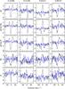 |
Fig. 1 Examples of LSD Stokes V (black) and N (blue) profiles taken at four typical rotational phases and for the five different line masks. The y-axis has been multiplied by 104. |
3. Magnetic field measurements
3.1. Magnetic Zeeman signatures
For each observation, we applied the least-squares deconvolution (LSD) technique (Donati et al. 1997) to the photospheric spectral lines in each echelle spectrum (wavelength domain from 3750 to 10 500 Å) to construct a single profile with an increased S/N. In that way, the Zeeman signature induced by the presence of a magnetic field is clearly visible in the high S/N LSD Stokes V profiles, as seen in Figs. 1 and 3. To compute the LSD profiles, we made use of five different line masks created from the Kurucz atomic database and ATLAS 9 atmospheric models of solar abundance (Kurucz 1993). We used one mask containing 335 photospheric He and metal lines of various chemical elements (all lines hereafter), one mask with all 268 metal lines (all but He lines), one mask with all He and metal lines except the N lines (313 lines, all but N lines), one mask containing 67 He lines, and finally one mask containing 22 N lines. For each spectral line, the mask contains the wavelength, depth, and Landé factor, to be used by the LSD code. The depths were modified so that they correspond to the depth of the observed spectral lines. Lines whose Landé factor is unknown were excluded. The average S/N of the LSD Stokes V profiles ranges from 5000 (mask with N-only lines) to 14 000 (mask with all lines) according to the number of lines used.
In Fig. 1, we compare LSD Stokes V and N profiles computed for different masks for typical rotation phases. The absence of significant signatures in the null spectra of all our observations indicates that owing to our short exposures, none of our measurements has been polluted by stellar pulsations. All the LSD Stokes V and I profiles, computed for the mask with all but He lines, are shown in Fig. 3. A magnetic Zeeman signature is present in almost all observations.
To statistically quantify the detection of a magnetic field in each of the Stokes V profile, we used the false alarm probability (FAP) of a signature in the LSD Stokes V profile inside the LSD line, compared to the mean noise level in the LSD Stokes V measurement outside the line. We adopted the convention defined by Donati et al. (1997): if FAP < 0.001%, the magnetic detection is definite, if 0.001% < FAP < 0.1% the detection is marginal, otherwise there is no magnetic detection. The type of detection for each measurement is reported in Table A.2. We find that 74 of our 82 measurements exhibit a definite detection, while three measurements show a marginal detection, and there is no detection in five of them.
3.2. Longitudinal magnetic field
We used the centre-of-gravity method on the LSD Stokes V and I profiles (Rees & Semel 1979; Wade et al. 2000) to compute the line-of-sight component of the magnetic field integrated over the visible stellar surface, which is called the longitudinal magnetic field and is written as ![Mathematical equation: \begin{equation} B_l=(-2.14 \times 10^{11} ~{\rm G})\frac{\int v V(v) {\rm d}v}{\lambda g c \int [1-I(v)]{\rm d}v}, \end{equation}](/articles/aa/full_html/2016/03/aa27751-15/aa27751-15-eq21.png) (1)where λ, in nm, is the mean, S/N-weighted wavelength, c is the velocity of light in the same units as the velocity v, and g is the mean, S/N-weighted value of the Landé factors of all lines used to construct the LSD profile. We used λ = 482 nm and g = 1.22 for the mask including all lines, all but He lines, and all but N lines. We used λ = 481 nm and g = 1.21 for the mask with He-only lines, and λ = 491 nm and g = 1.20 for the mask with N-only lines. The integration limits were chosen to be large enough to cover the width of the line but also small enough to avoid artificially increased error bars due to noisy continuum. A range of 23 and 20 km s-1 around the line centre was adopted when including the He lines or not, respectively.
(1)where λ, in nm, is the mean, S/N-weighted wavelength, c is the velocity of light in the same units as the velocity v, and g is the mean, S/N-weighted value of the Landé factors of all lines used to construct the LSD profile. We used λ = 482 nm and g = 1.22 for the mask including all lines, all but He lines, and all but N lines. We used λ = 481 nm and g = 1.21 for the mask with He-only lines, and λ = 491 nm and g = 1.20 for the mask with N-only lines. The integration limits were chosen to be large enough to cover the width of the line but also small enough to avoid artificially increased error bars due to noisy continuum. A range of 23 and 20 km s-1 around the line centre was adopted when including the He lines or not, respectively.
The values for the longitudinal magnetic field Bl and null Nl measurements are reported in Table A.2 for the different masks used. The Bl-values vary between about −25 and 10 G. The error bars are typically around 2.5, 3.5, 3.0, 3.1, and 6.5 G when using all, all but He, all but N, He, and N lines. It can be compared to the mean error bar of ~29 G for the Musicos Bl-values from Neiner et al. (2003a). Phase diagrams of the longitudinal magnetic field for the rotation period are shown in Fig. 2.
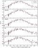 |
Fig. 2 Longitudinal magnetic field values plotted in phase with Prot = 5.370447 d and HJD0 = 2 446 871.89 d for the different groups of lines (from top to bottom: all photospheric He and metal lines, all photospheric lines except He lines, all photospheric lines except N lines, He-only lines, and N-only lines). A fit of the data for a dipole model (red line) is shown in each panel. |
4. Magnetic field modelling
4.1. Longitudinal field modelling
Assuming a centred dipole field and following Borra & Landstreet (1980), the magnetic obliquity angle β is constrained by the observed ratio Bl min/Bl max = cos(i − β) / cos(i + β) for a given stellar inclination angle i. The polar field Bpol is then deduced from B0 ± B = 0.283 ∗ Bpolcos(β ± i), where B0 and B are the constant and amplitude of a sine fit to the phase-folded Bl values, respectively (red lines in Fig. 2).
We adopt an inclination angle i of 30° deduced from modelling the LSD Stokes profiles (see Sect. 4.2), which is also obtained from our Zeeman-Doppler imaging (ZDI) modelling presented in Sect. 4.3. The results of a dipole fit on the longitudinal magnetic field values are reported in Table 1, considering the different groups of lines shown in Fig. 2. For example, for the mask using all but He lines, we obtain β = 104° and Bpol = 149 G, with an error of 1 deg and 5 G, respectively. We note that, even if the B0 and B-values are slightly different when considering the different masks, we get almost the same ratio Bl min/Bl max in all cases, so that the deduced β-value is the same for a given inclination angle i. What differs, depending on the adopted mask, is the Bpol-value, which amounts to 158 G at maximum. Different chemical elements probe different layers of the star and have different distributions at the surfaces. Therefore, the measured longitudinal field value for a given element differs from another element, which translates into different Bpol-values.
In Table 1, Δφ denotes the phase shift of the dipole fits compared to the ephemeris (Prot = 5.370447 d and HJD0 = 2 446 871.89 d) determined from the UV data by Neiner et al. (2003a). This ephemeris corresponds to the epoch of minimum in EW of UV C iv, Si iv, and N v lines (see their Fig. 2). Depending on the mask used, a phase shift between 0.020 and 0.033 is obtained. The errors of 0.054 d on HJD0 and of 0.000078 d on the rotation period allow for a phase shift up to ~0.07 between the old UV data and our recent Narval data, so that the dipole fits are compatible with the ephemeris derived from the UV data.
Results of a dipole fit on the longitudinal magnetic field values using the five groups of lines.
Magnetic field configuration obtained by modelling LSD Stokes profiles for a mask, including all but He lines, with a centred or off-centred oblique dipole magnetic field.
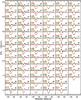 |
Fig. 3 Centred (solid red line) and off-centred (dashed green line) dipole field models superimposed on the LSD Stokes V profiles (thin solid black lines) for all phases of observation and using all but He lines, and the corresponding modelled (dashed red line) and observed (dotted black line) LSD Stokes I profiles. Above each profile, the rotation phase is indicated on the left and the number of the polarimetric sequence is indicated on the right. Typical error bars are shown next to each Stokes V profile. |
4.2. Modelling the LSD Stokes profiles
We also determined the magnetic configuration of ζ Cas by fitting synthetic LSD Stokes V and I profiles to the observed profiles for a centred dipole oblique rotator model. The free parameters of the model are the stellar inclination angle i (in degrees), the magnetic obliquity angle β (in degrees), and the dipole magnetic intensity Bpol (in Gauss). Afterwards, we checked whether a better fit is obtained with a dipole off-centred along the magnetic axis by a distance d (in stellar radius). A distance d = 0 corresponds to a centred dipole and d = 1 corresponds to a centre of the dipole at the surface of the star.
In our model, we use Gaussian local intensity profiles with a width calculated using the resolving power of Narval, a macroturbulence value of 2 km s-1, and a vsini of 20 km s-1. The depth is determined by fitting the observed LSD Stokes I profiles. The local Stokes V profiles are calculated assuming the weak-field case and using the weighted mean Landé factor and wavelength of the lines derived from the LSD mask (see Sect. 3.2). The synthetic Stokes V profiles are obtained by integrating over the visible stellar surface by using a linear limb darkening law with a parameter equal to 0.3. The Stokes V profiles are then normalised to the intensity continuum.
By varying the free parameters mentioned above, we calculated a grid of Stokes V profiles for each phase of observation for the rotation period Prot = 5.370447 d and the reference date HJD0 = 2 446 871.89 corresponding to the time of minimum equivalent width of the wind-sensitive UV line, used in Neiner et al. (2003a). In our fitting procedure, a phase shift compared to the UV ephemeris ΔΨ is allowed. We applied a χ2 minimisation to determine the model that best matches our 82 observed profiles simultaneously. The fitting was applied to observed LSD profiles obtained with all but He lines. We did not model the LSD Stokes profiles for the masks including He lines because a Gaussian intrinsic profile is not suited in those cases. The fitting to LSD profiles computed with the nitrogen lines led to similar parameter values as when using all but He lines, however with larger error bars, as expected from the lower S/N.
The parameter values obtained for a centred and off-centred model are listed in Table 2. The polar field strength obtained is of the order of 100 G, i is about 30°, and β around 105°. The values of the phase shift ΔΨ of <0.08 remains compatible with the ephemeris deduced from the UV data. The errors on the model parameters were determined with the help of the Minuit library, a physics analysis tool for function minimisation developed at conseil européen pour la recherche nucléaire (CERN1). The algorithm consists in varying a parameter at a time, and the three or four other parameters are held fixed to find the two values of the parameter for which the χ2 function is equal to its minimum (with respect to all parameters) plus a constant equal to 9 for 3σ errors. This algorithm takes into consideration the non-linearities of the χ2 function with respect to its parameters, i.e. the deviation of the χ2 profile from a perfect parabola at its minimum. Therefore, it provides slightly asymmetrical errors (not visible within our precision however). We checked that determining the errors for each parameter independently is justified by computing the Hessian matrix. We indeed find that the correlation terms are small.
The small value of the decentring parameter d along with the only slightly better reduced χ2-values for the off-centred cases imply that our data are fully consistent with a dipolar magnetic field at the centre of the star. Figure 3 shows the comparison between the observed and synthetic LSD V and I profiles for a centred and off-centred dipole for all phases of observation.
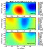 |
Fig. 4 Magnetic map of ζ Cas. The three panels illustrate the field components in spherical coordinates (from top to bottom: radial, azimuthal, meridional). The magnetic field strength (colour scale) is expressed in Gauss. The vertical ticks on top of the radial map show the phases of observations. |
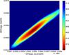 |
Fig. 5 Map of the mean surface magnetic field in Gauss in the differential rotation parameter plane. |
4.3. Zeeman-Doppler imaging
To determine the surface map of the magnetic field, we also used the ZDI technique (Donati & Brown 1997) following the procedure presented in Petit et al. (2010) and using the LSD Stokes profiles for all but He lines. In this procedure, the model assumes a constant Stokes I profile, which is not the case for ζ Cas. To avoid artefacts in the magnetic map due to the deformed intensity profiles, the spherical harmonic expansion was restricted to ℓ< 3. The best model has a reduced χ2 of 1.83 and is obtained for a stellar inclination of 30°. The corresponding ZDI map is shown in Fig. 4: the radial, azimuthal, and meridional components are shown. We find that the field has a simple configuration, compatible with an oblique dipole field, as expected for these kinds of stars. The mean field strength at the surface amounts to 82 G and the maximum field strength is 148 G at a latitude of 23°.
As a result of our very good phase coverage and our long time base of observations, we can measure the surface differential rotation of the star with high accuracy. To this end, we used the method developed by Petit et al. (2002), assuming a simplified solar rotation law Ω(ℓ) = Ωeq − dΩsin2ℓ, where Ω(ℓ) is the rotation rate at latitude ℓ, Ωeq is the rotation rate of the equator and dΩ is the difference in rotation rate between the pole and equator. As shown in Fig. 5, we obtain Ωeq = 1.16999 ± 0.00002 rad d-1 and dΩ = −0.0002 ± 0.0004 rad d-1. The parameter dΩ is found to be compatible with zero, which means that our Narval data are fully compatible with a solid body rotation at the surface, given the very low error bar. If differential rotation is present at a level below our detection threshold, our result is in favour of an anti-solar differential rotation, meaning that the pole would rotate faster than the equator.
4.4. Comparison of the modelling results
The best ZDI model is obtained for a stellar inclination of 30°, which is in perfect agreement with the value derived from our forward modelling (Sect. 4.2). In addition, the β angle (105°) obtained from the Bl values is similar to that deduced from the LSD Stokes modelling. However, the Bpol value found from fitting the LSD Stokes profiles (around 100 G, see Table 2) is lower than the value obtained from the Bl values or from the ZDI models, which are both compatible (around 150 G). However, one can consider an uncertainty of a factor of 2 on the magnetic strength reconstructed through ZDI (Vidotto et al. 2014).
For their magnetic field modelling, Neiner et al. (2003a) used an inclination angle i of 18° ± 6° while we obtained i ~ 30°. Their value was computed from Prot, vsini = 17 ± 3 km s-1 and a stellar radius of R = 5.9 ± 0.7 R⊙. The inclination angle adopted in Neiner et al. (2003a) is underestimated, because their vsini value was underestimated. Our spectra of higher precision led to vsini = 20 ± 3 km s-1, also obtained by Nieva & Przybilla (2012), which is compatible with our value of i ~ 30°. We conclude that a dipole oblique rotator model with i ~ 30°, β ~ 105° and Bpol ~ 100–150 G reproduces our spectropolarimetric measurements.
5. Discussion
5.1. Weak magnetic fields among B-type stars
Current spectropolarimetric data give us new insights about main-sequence stars with radiative envelopes (see Briquet 2015 for a review). Among intermediate-mass stars, there is evidence for two classes of magnetism: the Ap-like strong magnetism and the Vega-like ultra-weak magnetism. For the first group, the observed field is always higher than a threshold of 100 G for the longitudinal field, which corresponds to a polar field strength higher than 300 G (Aurière et al. 2010). In the second group, sub-Gauss longitudinal fields have been convincingly detected (Lignières et al. 2009; Petit et al. 2010; Blazère et al. 2016). Between both groups, no star is observed and one speaks of a magnetic desert (Lignières et al. 2014).
This raises the question of whether this dichotomy also holds for higher mass stars of spectral type O and B. For the latter, there are Bp stars, an extension of the Ap stars, i.e. stars with a typical polar strength of the order of kiloGauss, but no ultra-weak field has been observed so far. In fact, for massive stars, detecting fields with a longitudinal component below 1 Gauss requires the co-addition of even more high-resolution spectropolarimetric data than for A stars to reach the necessary S/N. This has only been attempted for two stars so far: γ Peg (Neiner et al. 2014b) and ι Her (Wade et al. 2014); hence, further investigation to search for Vega-like fields in OB stars is underway (Neiner et al. 2014a). Moreover, evidence for fields with intermediate polar strength of the order of tens or a couple hundred Gauss (weak fields) is increasingly observed in OB stars. So far, such weak fields have been observed in HD 37742 (ζ OriAa) (Blazère et al. 2015a,b), τ Sco (Donati et al. 2006), ϵ CMa (Fossati et al. 2015), and β CMa (Fossati et al. 2015). However, most of these targets are rather special: ζ OriAa is a young O supergiant and ϵ CMa is an evolved B star at the end of the main sequence. The increased radius of evolved stars explains their weak field compared to main-sequence stars because of magnetic flux conservation. In addition, τ Sco has a complex field, therefore the disk-integrated field is weaker because of cancellation effects on the visible surface hemisphere. β CMa seems to be a more normal B star, but it has not been studied in detail yet, so that its polar field strength is not clearly known. Our study of ζ Cas thus provides the first definite case of a weak polar field in a normal B star, based on a large amount of data that allows for modelling of its magnetic field configuration. As already pointed out in Fossati et al. (2015), our finding indicates a possible lack of a magnetic desert in massive stars, contrary to what is observed in main-sequence A-type stars or a field strength threshold in massive stars lower than that observed in intermediate-mass stars. In any case, ζ Cas exhibits the lowest polar field observed so far in a main-sequence B-type star.
5.2. Evidence for solid-envelope rotation
As discussed in Mathis & Neiner (2015) and Neiner et al. (2015b), there is increasing theoretical and observational evidence that the magnetic fields observed at the surface of intermediate and high-mass stars are remnants of an early phase of the life of the star. They are called fossil fields and reside inside the star without being continuously renewed. Furthermore, these magnetic fields deeply modify the transport of angular momentum and the mixing of chemicals. Above a critical field limit, the fields enforce a uniform rotation along field lines and mixing is inhibited (Mathis & Zahn 2005; Zahn 2011). The inhibition of mixing in the radiative zone by a magnetic field has been observed in the β Cep star V2052 Oph using the combination of spectropolarimetry and asteroseismology (Neiner et al. 2012a; Briquet et al. 2012). For the latter, the field strength observed (Bpol ~ 400 G) is six to ten times higher than the critical field limit needed to inhibit mixing as determined from theory.
As in Briquet et al. (2012), we determined the critical field strength at the surface Bcrit,surf for ζ Cas above which mixing is suppressed. In the criterion by Zahn (2011), one makes use of the time already spent by ζ Cas on the main sequence t, its radius R and mass M, as well as the surface rotation velocity. With i = 30° ± 1°, vsini = 20 ± 3 km s-1, and Prot = 5.37045 d, we have veq = 40 ± 7.5 km s-1 and R = 4.2 ± 0.8 R⊙. To estimate t and M, we computed main-sequence stellar models accounting for Teff = 20750 ± 200 K and log g = 3.80 ± 0.05 dex (Nieva & Przybilla 2012), within 3σ. To this end, we used the evolutionary code CLÉS (Code Liégeois d’Évolution Stellaire; Scuflaire et al. 2008) with the input physics described in Briquet et al. (2011). The hydrogen mass fraction X is set to 0.7. Allowing a core overshooting parameter value αov between 0 and 0.4 (expressed in local pressure scale heights) and a metallicity between 0.01 and 0.02, we obtain M ∈ [ 6.7,9.5 ] M⊙, R ∈ [ 4.5,7.6 ] R⊙, and t ∈ [ 19,40 ] Myr. If we limit to R ∈ [ 4.5,5.0 ] R⊙ to be compatible with the observational constraints on the stellar radius, we obtain M ∈ [ 6.7,8.0 ] M⊙, t ∈ [ 22,40 ] Myr, and log g ∈ [ 3.88,3.95 ]. Furthermore, if we set αov = 0, we get M ∈ [ 7.1,8.0 ] M⊙, t ∈ [ 22,29 ] Myr, and log g ∈ [ 3.89,3.95 ].
We found that the mean critical field strength in the radiative zone for suppressing differential rotation in this star is Bcrit = 45 G according to the criterion from Eq. (3.6) in Zahn (2011). According to the ratio (30) between internal and surface fields derived by Braithwaite (2008, see Fig. 8 therein), this corresponds to a critical field strength at the surface of Bcrit,surf = 1.5 G.
Considering that the observed field strength is 100−150 G, we expect rigid envelope rotation and no core overshooting for ζ Cas. We point out that the adopted criterion by Zahn (2011) is applicable only in the case of a magnetic obliquity angle β = 0, while ζ Cas has a large obliquity. Therefore, our result needs to be confirmed whenever a similar critical field criterion taking the obliquity angle into account is available (Neiner et al. 2015a; Mathis et al., in prep.). Nevertheless, the conclusion still holds when considering another criterion from Eq. (22) defined by Spruit (1999), which does take obliquity into account and yields Bcrit,surf< 35 G. Therefore, it is likely that the envelope of the star rotates uniformly. The above two criteria could also be influenced by the effect of waves, but this has never been studied. Therefore, we conclude that our study provides the first evidence for a solid body rotation in the envelope of a weak-field B-type star, but that this conclusion must be confirmed in the future with more elaborated critical field criteria.
5.3. Surface N-enrichment in early B-type stars
Early B-type stars are ideal indicators for present-day cosmic abundances (Nieva & Przybilla 2012) but, in a fraction of them, the stellar surface is found to be enriched with the products from hydrogen burning such as nitrogen (e.g. Morel et al. 2006). This is the case of ζ Cas. An explanation of the surface enrichment of certain chemical species is that internal mixing can lead to the dredge up of some core-processed CNO material. The usual interpretation is that rotationally induced mixing is responsible for the N-enrichment observed in massive stars (Meynet & Maeder 2000). Such a mixing is enhanced when magnetic braking occurs in models with interior differential rotation (Meynet et al. 2011) and the predicted N-enrichments depend on the rotation velocity, but also on the mass, age, binarity, metallicity, and magnetic field (Maeder & Meynet 2015). As discussed in the previous section, we proved that the envelope of ζ Cas rotates as a solid body. Therefore, the nitrogen overabundance in its stellar surface cannot be explained by rotationally induced mixing. This conclusion was also reached for the other magnetic N-rich β Cep pulsator V2052 Oph. For this star, an asteroseismic study showed that the stellar models reproducing the observed pulsational behaviour do not have any convective core overshooting and the observed fossil magnetic field is strong enough to inhibit interior mixing and enforce rigid rotation in the envelope (Briquet et al. 2012; Neiner et al. 2012a).
A surface N-enhancement linked to binarity (Langer 2008) is also ruled out by our observations for both ζ Cas and V2052 Oph. Therefore, yet another mechanism must be invoked to explain the abundance peculiarity. As discussed in Aerts et al. (2014), recent studies suggest that internal gravity waves might also play a role to account for the surface abundances. Indeed, theoretical and numerical simulations show that large-scale, low-frequency internal gravity waves are excited by the convective core and can transport angular momentum (Mathis 2013; Rogers et al. 2013). Such waves were revealed by high-precision, space-based CoRoT photometric data in several Be (Neiner et al. 2012b) and O-type stars. For the latter, a red noise power excess of physical origin was detected by Blomme et al. (2011) and then interpreted as internal gravity waves by Aerts & Rogers (2015). Clearly, such waves are present in massive stars and their transport modify the mixing in their radiative zone. Contrary to the case of solar-like stars (Press 1981; Schatzman 1996), the chemical transport that such waves induce in massive stars remains to be computed, so that a comparison between theoretical predictions and observations is currently not possible. However, our observational study of ζ Cas leads us to conclude that the most likely explanation for the nitrogen enrichment at its surface is the transport of chemicals from the core to the surface by internal gravity waves.
Several authors (Shiode et al. 2013; Rogers et al. 2013; Lee et al. 2014) have already demonstrated, thanks to analytical work or simulations, that the amplitude of these waves is sufficient to propagate to the surface and thus transport angular momentum and chemicals. Internal gravity waves propagate in the radiation zone and deposit or extract, depending on whether they are prograde or retrograde, angular momentum at the location where they are dissipated (Goldreich & Nicholson 1989; Zahn et al. 1997). Assuming the convective core rotates faster than the radiative envelope, the net angular momentum transport leads to an acceleration of surface layers (Lee et al. 2014). In the case of ζ Cas, we showed that rotation is likely uniform in the envelope because of the presence of the magnetic field. However, the rotation of the core could be higher or lower than the rotation of the envelope, and waves could locally increase differential rotation just below the surface.
Moreover, the magnetic field transforms gravity waves into magneto-gravity waves. However, if the frequency of the waves are higher than the Alfvén frequency, the properties of the waves are only slightly modified by a weak magnetic field, such as that observed in ζ Cas (Mathis & de Brye 2012; Mathis & Alvan 2013). In particular, radiative damping increases with the magnetic field strength; the angular momentum transport by waves thus becomes an inverse function of the field strength (Mathis & de Brye 2012). However, the weak magnetic field of ζ Cas does not hamper transport by waves much.
6. Summary
With the aim of better constraining the magnetic field configuration of ζ Cas, we made use of 82 Narval spectropolarimetric data well distributed over the accurately known rotation cycle of this N-rich magnetic B-type pulsator. Zeeman signatures typical of the presence of a magnetic field are seen in almost all LSD Stokes V profiles, while the diagnosis null spectra do not show any signature. This confirms that the signatures are of magnetic origin.
To model the magnetic field, we considered a dipole oblique rotator model and we fitted both the longitudinal measurements and the LSD Stokes V and I profiles to derive the parameter values of the model. Besides this forward approach, we also used the ZDI method to derive the surface map of the magnetic field of the star. Our magnetic modelling leads to a stellar inclination angle i of 30°, a magnetic obliquity angle β of 105°, and a polar field strength Bpol of 100−150 G.
Although weak magnetic fields have already been reported for several massive stars, ζ Cas is the only firmly established case of a weak polar field in a normal B star and exhibits the lowest field observed so far in a massive main-sequence star. We also point out that ζ Cas has a polar field strength in the range where a so-called magnetic desert between about 1 G and 300 G is observed for intermediate-mass stars. This indicates that either there is no magnetic desert for massive stars or such a desert is less extended for massive stars than for intermediate-mass stars.
In addition, owing to our intensive dataset, our ZDI modelling allowed us to test whether the star shows surface differential rotation. Besides that, a theoretical criterion was used to determine the critical field strength above which mixing is suppressed. Both approaches led to the conclusion that ζ Cas rotates as a solid body in the envelope. Indeed, our Narval data prove that there is no surface differential rotation, while theory predicts that the magnetic field enforced an interior rigid rotation in the radiative zone.
To explain the nitrogen enrichment that is observed at the surface of a fraction of massive stars, and in ζ Cas, the proposed explanations are rotationally induced mixing, a binarity origin, or a pulsational cause. For ζ Cas, the first two hypothesis are ruled out as a result of our study since interior differential rotation is excluded and there is no evidence of binarity in the high-resolution high S/N spectropolarimetry taken on a long time base. Therefore, the pulsational origin remains the most convincing explanation for the observed peculiarity. ζ Cas is likely N-rich because of the transport of core-processed CNO material from the core to the surface by internal gravity waves.
Acknowledgments
The authors would like to thank Stéphane Mathis for useful discussions. C.N. acknowledges support from the ANR (Agence Nationale de la Recherche) project Imagine. This research has made use of the SIMBAD database operated at CDS, Strasbourg (France), and of NASA’s Astrophysics Data System (ADS).
References
- Aerts, C., & Rogers, T. M. 2015, ApJ, 806, L33 [NASA ADS] [CrossRef] [Google Scholar]
- Aerts, C., Molenberghs, G., Kenward, M. G., & Neiner, C. 2014, ApJ, 781, 88 [NASA ADS] [CrossRef] [Google Scholar]
- Alecian, E., Kochukhov, O., Neiner, C., et al. 2011, A&A, 536, L6 [NASA ADS] [CrossRef] [EDP Sciences] [Google Scholar]
- Aurière, M., Wade, G. A., Lignières, F., et al. 2010, A&A, 523, A40 [NASA ADS] [CrossRef] [EDP Sciences] [Google Scholar]
- Blazère, A., Neiner, C., Bouret, J.-C., & Tkachenko, A. 2015a, in IAU Symp. 307, eds. G. Meynet, C. Georgy, J. Groh, & P. Stee, 367 [Google Scholar]
- Blazère, A., Neiner, C., Tkachenko, A., Bouret, J.-C., & Rivinius, T. 2015b, A&A, 582, A110 [NASA ADS] [CrossRef] [EDP Sciences] [Google Scholar]
- Blazère, A., Petit, P., Lignières, F., et al. 2016, A&A, 586, A97 [NASA ADS] [CrossRef] [EDP Sciences] [Google Scholar]
- Blomme, R., Mahy, L., Catala, C., et al. 2011, A&A, 533, A4 [NASA ADS] [CrossRef] [EDP Sciences] [Google Scholar]
- Borra, E. F., & Landstreet, J. D. 1980, ApJS, 42, 421 [NASA ADS] [CrossRef] [Google Scholar]
- Braithwaite, J. 2008, MNRAS, 386, 1947 [NASA ADS] [CrossRef] [Google Scholar]
- Briquet, M. 2015, EPJ, 101, 5001 [Google Scholar]
- Briquet, M., & Morel, T. 2007, Comm. Asteroseismol., 150, 183 [Google Scholar]
- Briquet, M., Aerts, C., Baglin, A., et al. 2011, A&A, 527, A112 [NASA ADS] [CrossRef] [EDP Sciences] [Google Scholar]
- Briquet, M., Neiner, C., Aerts, C., et al. 2012, MNRAS, 427, 483 [NASA ADS] [CrossRef] [Google Scholar]
- Briquet, M., Neiner, C., Leroy, B., Pápics, P. I., & MiMeS collaboration 2013, A&A, 557, L16 [NASA ADS] [CrossRef] [EDP Sciences] [Google Scholar]
- Donati, J.-F., & Brown, S. F. 1997, A&A, 326, 1135 [NASA ADS] [Google Scholar]
- Donati, J.-F., Semel, M., Carter, B. D., Rees, D. E., & Collier Cameron, A. 1997, MNRAS, 291, 658 [NASA ADS] [CrossRef] [MathSciNet] [Google Scholar]
- Donati, J.-F., Howarth, I. D., Jardine, M. M., et al. 2006, MNRAS, 370, 629 [NASA ADS] [CrossRef] [Google Scholar]
- Fossati, L., Castro, N., Morel, T., et al. 2015, A&A, 574, A20 [NASA ADS] [CrossRef] [EDP Sciences] [Google Scholar]
- Gies, D. R., & Lambert, D. L. 1992, ApJ, 387, 673 [NASA ADS] [CrossRef] [Google Scholar]
- Goldreich, P., & Nicholson, P. D. 1989, ApJ, 342, 1075 [NASA ADS] [CrossRef] [Google Scholar]
- Henrichs, H. F., de Jong, J. A., Donati, D.-F., et al. 2000, in Magnetic Fields of Chemically Peculiar and Related Stars, eds. Y. V. Glagolevskij, & I. I. Romanyuk, 57 [Google Scholar]
- Henrichs, H. F., Neiner, C., Schnerr, R. S., et al. 2009, in IAU Symp. 259, eds. K. G. Strassmeier, A. G. Kosovichev, & J. E. Beckman, 393 [Google Scholar]
- Henrichs, H. F., Kolenberg, K., Plaggenborg, B., et al. 2012, A&A, 545, A119 [NASA ADS] [CrossRef] [EDP Sciences] [Google Scholar]
- Hubrig, S., Briquet, M., Schöller, M., et al. 2006, MNRAS, 369, L61 [NASA ADS] [CrossRef] [Google Scholar]
- Hubrig, S., Briquet, M., De Cat, P., et al. 2009, Astron. Nachr., 330, 317 [NASA ADS] [CrossRef] [Google Scholar]
- Hubrig, S., Ilyin, I., Schöller, M., et al. 2011, ApJ, 726, L5 [NASA ADS] [CrossRef] [Google Scholar]
- Langer, N. 2008, in IAU Symp. 252, eds. L. Deng, & K. L. Chan, 467 [Google Scholar]
- Lee, U., Neiner, C., & Mathis, S. 2014, MNRAS, 443, 1515 [NASA ADS] [CrossRef] [Google Scholar]
- Lefever, K., Puls, J., Morel, T., et al. 2010, A&A, 515, A74 [NASA ADS] [CrossRef] [EDP Sciences] [Google Scholar]
- Lignières, F., Petit, P., Böhm, T., & Aurière, M. 2009, A&A, 500, L41 [NASA ADS] [CrossRef] [EDP Sciences] [Google Scholar]
- Lignières, F., Petit, P., Aurière, M., Wade, G. A., & Böhm, T. 2014, in IAU Symp. 302, eds. P. Petit, M. Jardine, & H. C. Spruit, 338 [Google Scholar]
- Maeder, A., & Meynet, G. 2015, in IAU Symp. 307, eds. G. Meynet, C. Georgy, J. Groh, & P. Stee, 9 [Google Scholar]
- Martins, F., Escolano, C., Wade, G. A., et al. 2012, A&A, 538, A29 [NASA ADS] [CrossRef] [EDP Sciences] [Google Scholar]
- Mathis, S. 2013, in EAS PS 63, eds. G. Alecian, Y. Lebreton, O. Richard, & G. Vauclair, 269 [Google Scholar]
- Mathis, S., & Alvan, L. 2013, in Progress in Physics of the Sun and Stars: A New Era in Helio- and Asteroseismology, eds. H. Shibahashi, & A. E. Lynas-Gray, ASP Conf. Ser., 479, 295 [Google Scholar]
- Mathis, S., & de Brye, N. 2012, A&A, 540, A37 [NASA ADS] [CrossRef] [EDP Sciences] [Google Scholar]
- Mathis, S., & Neiner, C. 2015, in IAU Symp. 307, eds. G. Meynet, C. Georgy, J. Groh, & P. Stee, 420 [Google Scholar]
- Mathis, S., & Zahn, J.-P. 2005, A&A, 440, 653 [NASA ADS] [CrossRef] [EDP Sciences] [Google Scholar]
- Meynet, G., & Maeder, A. 2000, A&A, 361, 101 [NASA ADS] [Google Scholar]
- Meynet, G., Eggenberger, P., & Maeder, A. 2011, A&A, 525, L11 [NASA ADS] [CrossRef] [EDP Sciences] [Google Scholar]
- Morel, T., Butler, K., Aerts, C., Neiner, C., & Briquet, M. 2006, A&A, 457, 651 [NASA ADS] [CrossRef] [EDP Sciences] [Google Scholar]
- Morel, T., Hubrig, S., & Briquet, M. 2008, A&A, 481, 453 [NASA ADS] [CrossRef] [EDP Sciences] [Google Scholar]
- Neiner, C., Geers, V. C., Henrichs, H. F., et al. 2003a, A&A, 406, 1019 [NASA ADS] [CrossRef] [EDP Sciences] [Google Scholar]
- Neiner, C., Henrichs, H. F., Floquet, M., et al. 2003b, A&A, 411, 565 [NASA ADS] [CrossRef] [EDP Sciences] [Google Scholar]
- Neiner, C., Alecian, E., Briquet, M., et al. 2012a, A&A, 537, A148 [NASA ADS] [CrossRef] [EDP Sciences] [Google Scholar]
- Neiner, C., Floquet, M., Samadi, R., et al. 2012b, A&A, 546, A47 [NASA ADS] [CrossRef] [EDP Sciences] [Google Scholar]
- Neiner, C., Folsom, C. P., & Blazere, A. 2014a, in SF2A-2014: Proceedings of the Annual meeting of the French Society of Astronomy and Astrophysics, eds. J. Ballet, F. Martins, F. Bournaud, R. Monier, & C. Reylé, 163 [Google Scholar]
- Neiner, C., Monin, D., Leroy, B., Mathis, S., & Bohlender, D. 2014b, A&A, 562, A59 [NASA ADS] [CrossRef] [EDP Sciences] [Google Scholar]
- Neiner, C., Tkachenko, A., & MiMeS Collaboration. 2014c, A&A, 563, L7 [NASA ADS] [CrossRef] [EDP Sciences] [Google Scholar]
- Neiner, C., Briquet, M., Mathis, S., & Degroote, P. 2015a, in IAU Symp. 307, eds. G. Meynet, C. Georgy, J. Groh, & P. Stee, 443 [Google Scholar]
- Neiner, C., Mathis, S., Alecian, E., et al. 2015b, in IAU Symp., 305, 61 [Google Scholar]
- Nieva, M.-F., & Przybilla, N. 2012, A&A, 539, A143 [NASA ADS] [CrossRef] [EDP Sciences] [Google Scholar]
- Petit, P., Donati, J.-F., & Collier Cameron, A. 2002, MNRAS, 334, 374 [NASA ADS] [CrossRef] [MathSciNet] [Google Scholar]
- Petit, P., Lignières, F., Wade, G. A., et al. 2010, A&A, 523, A41 [NASA ADS] [CrossRef] [EDP Sciences] [Google Scholar]
- Press, W. H. 1981, ApJ, 245, 286 [NASA ADS] [CrossRef] [Google Scholar]
- Rees, D. E., & Semel, M. D. 1979, A&A, 74, 1 [NASA ADS] [Google Scholar]
- Rogers, T. M., Lin, D. N. C., McElwaine, J. N., & Lau, H. H. B. 2013, ApJ, 772, 21 [NASA ADS] [CrossRef] [Google Scholar]
- Sadsaoud, H., Le Contel, J. M., Chapellier, E., Le Contel, D., & Gonzalez-Bedolla, S. 1994, A&A, 287, 509 [NASA ADS] [Google Scholar]
- Schatzman, E. 1996, Sol. Phys., 169, 245 [NASA ADS] [CrossRef] [Google Scholar]
- Scuflaire, R., Théado, S., Montalbán, J., et al. 2008, Ap&SS, 316, 83 [NASA ADS] [CrossRef] [Google Scholar]
- Shiode, J. H., Quataert, E., Cantiello, M., & Bildsten, L. 2013, MNRAS, 430, 1736 [NASA ADS] [CrossRef] [Google Scholar]
- Silvester, J., Neiner, C., Henrichs, H. F., et al. 2009, MNRAS, 398, 1505 [NASA ADS] [CrossRef] [Google Scholar]
- Smith, M. A. 1980, in Nonradial and Nonlinear Stellar Pulsation, eds. H. A. Hill, & W. A. Dziembowski (Berlin: Springer Verlag), Lect. Notes Phys., 125, 60 [Google Scholar]
- Sódor, Á., De Cat, P., Wright, D. J., et al. 2014, MNRAS, 438, 3535 [NASA ADS] [CrossRef] [Google Scholar]
- Spruit, H. C. 1999, A&A, 349, 189 [NASA ADS] [Google Scholar]
- Vidotto, A. A., Gregory, S. G., Jardine, M., et al. 2014, MNRAS, 441, 2361 [NASA ADS] [CrossRef] [Google Scholar]
- Wade, G. A., Donati, J.-F., Landstreet, J. D., & Shorlin, S. L. S. 2000, MNRAS, 313, 851 [NASA ADS] [CrossRef] [Google Scholar]
- Wade, G. A., Folsom, C. P., Petit, P., et al. 2014, MNRAS, 444, 1993 [NASA ADS] [CrossRef] [Google Scholar]
- Zahn, J.-P. 2011, in IAU Symp. 272, eds. C. Neiner, G. Wade, G. Meynet, & G. Peters, 14 [Google Scholar]
- Zahn, J.-P., Talon, S., & Matias, J. 1997, A&A, 322, 320 [Google Scholar]
Appendix A: Journal of Narval/TBL observations and magnetic field measurements
Journal of Narval/TBL observations of ζ Cas. Column 1/8 indicates the number of the polarimetric sequence.
Magnetic field measurements of ζ Cas.
continued.
All Tables
Results of a dipole fit on the longitudinal magnetic field values using the five groups of lines.
Magnetic field configuration obtained by modelling LSD Stokes profiles for a mask, including all but He lines, with a centred or off-centred oblique dipole magnetic field.
Journal of Narval/TBL observations of ζ Cas. Column 1/8 indicates the number of the polarimetric sequence.
All Figures
|
Fig. 1 Examples of LSD Stokes V (black) and N (blue) profiles taken at four typical rotational phases and for the five different line masks. The y-axis has been multiplied by 104. |
| In the text | |
|
Fig. 2 Longitudinal magnetic field values plotted in phase with Prot = 5.370447 d and HJD0 = 2 446 871.89 d for the different groups of lines (from top to bottom: all photospheric He and metal lines, all photospheric lines except He lines, all photospheric lines except N lines, He-only lines, and N-only lines). A fit of the data for a dipole model (red line) is shown in each panel. |
| In the text | |
|
Fig. 3 Centred (solid red line) and off-centred (dashed green line) dipole field models superimposed on the LSD Stokes V profiles (thin solid black lines) for all phases of observation and using all but He lines, and the corresponding modelled (dashed red line) and observed (dotted black line) LSD Stokes I profiles. Above each profile, the rotation phase is indicated on the left and the number of the polarimetric sequence is indicated on the right. Typical error bars are shown next to each Stokes V profile. |
| In the text | |
|
Fig. 4 Magnetic map of ζ Cas. The three panels illustrate the field components in spherical coordinates (from top to bottom: radial, azimuthal, meridional). The magnetic field strength (colour scale) is expressed in Gauss. The vertical ticks on top of the radial map show the phases of observations. |
| In the text | |
|
Fig. 5 Map of the mean surface magnetic field in Gauss in the differential rotation parameter plane. |
| In the text | |
Current usage metrics show cumulative count of Article Views (full-text article views including HTML views, PDF and ePub downloads, according to the available data) and Abstracts Views on Vision4Press platform.
Data correspond to usage on the plateform after 2015. The current usage metrics is available 48-96 hours after online publication and is updated daily on week days.
Initial download of the metrics may take a while.