| Issue |
A&A
Volume 587, March 2016
|
|
|---|---|---|
| Article Number | A107 | |
| Number of page(s) | 9 | |
| Section | Atomic, molecular, and nuclear data | |
| DOI | https://doi.org/10.1051/0004-6361/201527669 | |
| Published online | 26 February 2016 | |
Rates of E1, E2, M1, and M2 transitions in Ni II⋆
School of Mathematics and Physics, Queen’s
University, Belfast,
BT7 1NN, Northern
Ireland
e-mail: This email address is being protected from spambots. You need JavaScript enabled to view it.
Received: 30 October 2015
Accepted: 15 December 2015
Abstract
Aims. We present rates for all E1, E2, M1, and M2 transitions among the 295 fine-structure levels of the configurations 3d9, 3d84s, 3d74s2, 3d84p, and 3d74s4p, determined through an extensive configuration interaction calculation.
Methods. The CIV3 code developed by Hibbert and coworkers is used to determine for these levels configuration interaction wave functions with relativistic effects introduced through the Breit-Pauli approximation.
Results. Two different sets of calculations have been undertaken with different 3d and 4d functions to ascertain the effect of such variation. The main body of the text includes a representative selection of data, chosen so that key points can be discussed. Some analysis to assess the accuracy of the present data has been undertaken, including comparison with earlier calculations and the more limited range of experimental determinations. The full set of transition data is given in the supplementary material as it is very extensive.
Conclusions. We believe that the present transition data are the best currently available.
Key words: atomic data / atomic processes
Full Table 4 and Tables 5−8 are only available at the CDS via anonymous ftp to cdsarc.u-strasbg.fr (130.79.128.5) or via http://cdsarc.u-strasbg.fr/viz-bin/qcat?J/A+A/587/A107
© ESO, 2016
1. Introduction
The greater efficiency of contemporary observational research facilities has led to the generation of huge quantities of observational data, which depend upon accurate and extensive atomic data for a range of processes for their meaningful interpretation. These observational efforts therefore require parallel theoretical efforts in order to determine the atomic parameters, including oscillator strengths and transition rates, at the accuracy required by astronomers.
The complex near-neutral Ni II ion is a member of the group of important iron-peak elements. Low-ionisation stages of these species are highly abundant in the astronomical environment, being commonly observed in a multitude of astrophysical sources including white dwarfs (Klein et al. 2011), evolved stars (Richardson et al. 2011), γ-ray bursts (Cucchiara et al. 2011; Vreeswijk et al. 2007), luminous blue variables (LBVs) (Davidson et al. 2001; Hartman et al. 2004), Seyfert galaxies (Véron-Cetty et al. 2006), quasi-stellar objects (Fynbo et al. 2010), and damped Lyα systems (DLAs; Dessauges-Zavadsky et al. 2006). There is therefore an on-going demand for accurate transition data among levels of Ni II.
This demand has inspired a number of experimental compilations over the past five decades. The first work in more recent years is by Ferrero et al. (1997) who presented transition probabilities for 59 ultraviolet (UV) lines in the spectral range λ2100−2600 Å.
The observational determinations of Zsargo & Federman (1998) followed. These authors presented a self-consistent set of relative f-values for 12 absorption resonance lines of the Ni II spectrum in the vacuum ultraviolet (VUV) spectral range λ1300−1750 Å. Comparison of these relative strengths with the compilation of Morton (1991) revealed good agreement for the stronger lines, but considerable differences for the weaker transitions.
Fedchak & Lawler (1999) reported absolute atomic transition probabilities for 59 UV and VUV lines of Ni II in the spectral range λ1700−2550 Å. It is important to note that in the work of Fedchak & Lawler (1999), the authors recommend that the relative f-values of Zsargó & Federman (1998) be put on an absolute scale by employing a reducing scaling factor of 0.534 (± 10%).
The work of Fedchak & Lawler (1999) was extended by the measurements of Fedchak et al. (2000), who reported seven relative absorption f-values for resonance transitions in Ni II. Three of the reported resonance transitions coincide with those of the 1999 analysis; however, Fedchak et al. (2000) stated that the later results are of somewhat improved accuracy.
A resonance transition neglected by Fedchak et al. (2000) was the 3d9
 transition at λ1317 Å. This transition was
re-evaluated in the more recent work of Dessauges-Zavadsky et al. (2006). The most recent experimental measurements of Ni II f-values are those of Jenkins
& Tripp (2006), with the derivation of
f-values for
the Ni II transitions at λ1317 Å and λ1370 Å. The f-value for the transition at
λ1317 Å was
found to be identical to that derived by Dessauges-Zavadsky et al. (2006), while the f-value for the transition at λ1370 Å was 0.76 times the
value of Zsargó & Federman (1998).
transition at λ1317 Å. This transition was
re-evaluated in the more recent work of Dessauges-Zavadsky et al. (2006). The most recent experimental measurements of Ni II f-values are those of Jenkins
& Tripp (2006), with the derivation of
f-values for
the Ni II transitions at λ1317 Å and λ1370 Å. The f-value for the transition at
λ1317 Å was
found to be identical to that derived by Dessauges-Zavadsky et al. (2006), while the f-value for the transition at λ1370 Å was 0.76 times the
value of Zsargó & Federman (1998).
An accurate atomic structure calculation for Ni II presents a formidable challenge to theorists. The complexity of the problem is primarily due to the open d-shell structure of the ionic system. Such an open shell arrangement gives rise to many LS states, some of which differ solely by the seniority quantum number of the 3d subshell and thus strong interaction between states is prevalent. Furthermore, the close spacing between many of the fine-structure levels makes their unique identification difficult because of the strong CI mixing, especially the levels associated with the 3d74s 4p configuration.
Early theoretical evaluations of Gruzdev (1962) and Mendlowitz (1966) reported intermediate coupling calculations of transition probabilities of 3d84p to 3d84s lines of Ni II. The Cowan code (Cowan 1967) calculations of Kurucz followed. Kurucz has completed a number of theoretical studies over the past two decades, culminating in compilations including Kurucz & Bell (1995) and Kurucz (2000). We note that the latter reference constitutes the most comprehensive theoretical analysis of structural atomic data for Ni II completed to date. The calculations of Kurucz & Bell (1995) are in reasonable agreement with the UV measurements of Fedchek & Lawler (1999). At VUV wavelengths, however, poor agreement is exhibited. Similarly, significant differences are found between the f-values determined by Kurucz & Bell (1995) and the laboratory measured values of Fedchak et al. (2000). These discrepancies perhaps highlight the inaccuracy of the former theoretical computation.
Fritzsche et al. (2000) have computed wavelengths and transition probabilities for all E1 transitions among the 3d9−3d84p and 3d84s−3d84p multiplets of Ni II, establishing a dataset comprising 450 emission lines. Multi-configuration Dirac-Fock (MCDF) wavefunctions were generated using GRASP2 (Grant et al. 1980) and the associated transition probabilities and lifetimes calculated using the relaxed-orbital REOS program (Fritzsche & Froese Fischer 1997). When compared with previously evaluated theoretical and experimental data, an accuracy of better than 25% for most strong lines was estimated; larger uncertainties are expected for weaker transitions. The oscillator strengths as derived from the transition probabilities of Fritzsche et al. (2000) were later compared to the experimental determinations of Jenkins & Tripp (2006). The theoretical f-value for the resonance transition at λ1317 Å was found to lie 18% higher than the experimental value. A difference of 13% was noted for the resonance line at λ1370 Å.
In this paper we present a new atomic structure calculation of the Ni II ion in order to yield a complete set of transition rates and oscillator strengths for the electric dipole (E1) transitions among all the 3d9, 3d84s, 3d74s2, and the 3d84p and 3d74s4p levels, calculated with an extensive set of configurations designed to provide data as accurately as possible within the constraints of our computer power. The limited extent of the available experimental measurements of Ni II transition data and the limited number of earlier theoretical compilations, in addition to some discrepancies evident among the published experimental and theoretical data, leaves a need for a large-scale CI calculation to support spectral analysis. This is further emphasized by Morton (2003) in his critical compilation of atomic data for resonance lines, where he expresses the need for improved calculations for Ni II. Transition data is also calculated, using the same wavefunctions, for E2, M1, and M2 transitions: the data is presented in the supplementary material
Radial function parameters.
2. Theoretical method
The present calculation was undertaken using the CIV3 code (Hibbert 1975; Hibbert et al. 1991) which
expresses the configuration interaction (CI) wave function in the intermediate coupling
scheme as 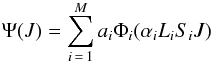 (1)In (1), Φi represents a
configuration state function (CSF), constructed from a common set of one-electron orbitals
of the form
(1)In (1), Φi represents a
configuration state function (CSF), constructed from a common set of one-electron orbitals
of the form 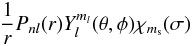 (2)where Y is a spherical harmonic,
χ is a spin
function (often denoted by α or β for
(2)where Y is a spherical harmonic,
χ is a spin
function (often denoted by α or β for  or
or  respectively) and the radial functions in
(2) are expressed in analytic form as linear combinations of normalised Slater orbitals
(STOs):
respectively) and the radial functions in
(2) are expressed in analytic form as linear combinations of normalised Slater orbitals
(STOs): 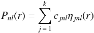 (3)and where the STOs take the form
![Mathematical equation: \begin{eqnarray} \eta_{jnl}(r)=\left[\frac {(2\xi_{jnl})^{2I_{jnl +1}}}{(2I_{jnl})!}\right]^{1/2} r^{I_{jnl}} \exp(-\xi_{jnl}r). \end{eqnarray}](/articles/aa/full_html/2016/03/aa27669-15/aa27669-15-eq31.png) (4)Also in (1), αi represents the angular
momentum coupling scheme and other necessary labelling, and ai is the corresponding
component of the eigenvector, associated with this wave function, of the diagonalised
Hamiltonian matrix whose typical element is Hij = ⟨ Φi |
H | Φj ⟩.
(4)Also in (1), αi represents the angular
momentum coupling scheme and other necessary labelling, and ai is the corresponding
component of the eigenvector, associated with this wave function, of the diagonalised
Hamiltonian matrix whose typical element is Hij = ⟨ Φi |
H | Φj ⟩.
If the eigenvalues (expressed as Ei) of the Hamiltonian
matrix are ordered to satisfy E1<E2<E3<...,
then  is a consequence of the Hylleraas-Undheim
theorem. These inequalities serve as a set of variational principles whereby the orbital
function parameters can be optimised on one or more eigenenergies of the Hamiltonian matrix,
and subject to the orthonormality conditions
is a consequence of the Hylleraas-Undheim
theorem. These inequalities serve as a set of variational principles whereby the orbital
function parameters can be optimised on one or more eigenenergies of the Hamiltonian matrix,
and subject to the orthonormality conditions
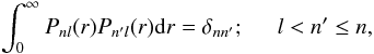 (5)so that the orbitals form an orthonormal set.
The Hamiltonian used in the optimisation process was simply the non-relativistic (LS
coupled) Schrödinger Hamiltonian. However, the Hamiltonian used to determine the final LSJ
wave functions, and therefore our oscillator strengths, consisted of the non-relativistic
Schrödinger Hamiltonian plus the following relativistic operators associated with the
Breit-Pauli approximation: mass-correction, Darwin and spin-orbit contributions, and a
one-electron approximation to the spin-other-orbit term. We found that this latter operator
gives almost identical energies to those obtained with the full spin-other-orbit operator.
(5)so that the orbitals form an orthonormal set.
The Hamiltonian used in the optimisation process was simply the non-relativistic (LS
coupled) Schrödinger Hamiltonian. However, the Hamiltonian used to determine the final LSJ
wave functions, and therefore our oscillator strengths, consisted of the non-relativistic
Schrödinger Hamiltonian plus the following relativistic operators associated with the
Breit-Pauli approximation: mass-correction, Darwin and spin-orbit contributions, and a
one-electron approximation to the spin-other-orbit term. We found that this latter operator
gives almost identical energies to those obtained with the full spin-other-orbit operator.
2.1. Optimisation of the radial functions
All the radial functions and associated orbital parameters adopted in the present analysis have been optimised using LS coupling only. Trial optimisations incorporating relativistic operators (specifically the Breit-Pauli mass correction and Darwin terms) resulted in only small changes in the mean radii of the radial functions, so we reverted to those optimised in LS coupling only.
Initially, we chose the 1s, 2s, 2p, 3s, 3p, and 3d orbitals to be the Hartree-Fock functions of the Ni II ground state (3d92D) given by Clementi & Roetti (1974). An additional four orbitals, 4s, 4p, 4d, and 4f were optimised on the energies of various states. The 4s and 4p orbitals were optimised as spectroscopic orbitals on the energy eigenvalues of the 3d8(3F)4s 2F and 3d8(3F)4p 4D° states respectively. Five (rather than the minimum of four required by (5)) STOs were included in the 4s orbital to allow some additional flexibility in the form of the radial function. One particular difficulty in undertaking calculations of near-neutral elements in the iron group is that the 3d function of the ground state is not optimal for states containing 3d8 or 3d7. Accordingly, the 4d orbital was optimised on the 3d8(1D)4s 2D eigenvalue using configurations [3d84s + 3d74s4d]. The optimal 3d orbital for this 2D state is then described by a linear combination of the Hartree-Fock 3d function of the ground state and the optimised 4d correcting function. In the present calculation, valence correlation plays an important role. A major component of valence correlation is provided by 3d2→ 4f2 replacements in key configurations. Hence we optimised our 4f orbital function on the energy of the 3d92D ground state using configurations [3d9 + 3d84s + 3d74s2 + 3d74f2 + 3d64s4f2 + 3d54s24f2]. Additionally, although originally optimised as a correcting function, the 4d orbital can be used in the role of a correlation orbital. The inclusion of further correlation orbitals would cause a substantial increase in the number of CSFs. Trial calculations suggested to us that this did not warrant the appreciable extension to the computational effort; as we shall see in a later section, even the orbitals up to n = 4 resulted in a very large set of CSFs. We refer to the use of this set of orbitals as Calculation A. The optimised radial function parameters of 3d and the n = 4 orbitals are shown in Table 1.
We found that, in the calculation of energy levels, the energy order of a few of the states, particularly some of 3d8nl, did not match those of the experimental energy level data. So we also undertook Calculation B, in which we started with the orbitals used in Calculation A, but reoptimised 3d on the energy of 3d8(3F)4p 2D°, and then 4d on the ground state using configurations 3d9 and 3d84d. Additionally, we included 5s as a correcting orbital for 4s, and 5p and 6p for the 4p. Again the parameters of the new orbitals are shown in Table 1.
2.2. Choice of configurations
In addition to the process of orbital optimisation, it is necessary to make a careful selection of associated basis CSF sets for inclusion in the CI expansions of the wavefunctions (1). In Calculaton A, the configurations required for the construction of the CSFs were generated by permitting all single and double orbital replacements from the outer subshells (beyond 3p) of a reference set comprising 3d9, 3d84s, 3d74s2 even parity and 3d84p, 3d74s4p odd parity configurations, to all of the available orbitals. We also found that opening the 3s and 3p subshells had a favourable effect on the theoretical transition energies and so, as a second stage, we allowed single and double orbital replacements from these subshells also. Thus only a 1s22s22p6 core was retained in all the CSFs.
The ensuing sets of CSFs associated with the even parity symmetries are of manageable size, but some of those for the odd parity symmetries are much larger. Although our analysis certainly permits CI expansions of considerable size, many of the CSFs proved to have very small mixing coefficients and their omission made very little difference either to the energy eigenvalues or to the mixing coefficients of the remaining CSFs. So before performing an LSJ calculation, we omitted those CSFs for which | ai | < 0.001 in all relevant eigenvalues of the odd parity LS states under investigation in this work. A computationally manageable calculation was thus achieved without losing significant accuracy.
The approach in Calculation B was slightly different. Again, we generated CSFs by permitting all single and double replacements from the same reference set which was used in Calculation A, but we augmented those only by CSFs arising from the replacements 3s → 3d, 3s2 → 3d2, 3p2 → 3d2. However, we did not exclude CSFs with small mixing coefficients.
2.3. Inclusion of relativistic effects
For the LSJ calculations, we have incorporated relativistic effects via the Breit-Pauli
approximation. CIV3 includes the spin-independent one-body Darwin and mass correction
terms, which affect only the overall energy of each LS coupled term, and three
spin-dependent fine-structure terms, representing the one-body spin-orbit (SO) interaction
and the two-body spin-other-orbit (SOO) and spin-spin (SS) interactions, which split each
LS state into separate J-dependent levels. However, in our work, due to the extensive CSF
sets employed, the calculation of the SOO and SS matrix elements would have proved
prohibitively time-consuming. For systems such as Ni II with a several closed subshells,
Hibbert & Bailie (1992) showed that very little
accuracy is lost by neglecting the spin-spin term and approximating the SO and SOO terms
by a modified spin-orbit operator:
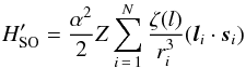 (6)where ζ(l) is a
parameter that depends only on the l-value of the interacting electrons in the
Breit-Pauli Hamiltonian matrix element, and chosen to reproduce specific matrix elements
of the full SO and SOO operators for certain key CSFs. This process is then independent of
the numbers or types of the CSFs included in the CI expansions.
(6)where ζ(l) is a
parameter that depends only on the l-value of the interacting electrons in the
Breit-Pauli Hamiltonian matrix element, and chosen to reproduce specific matrix elements
of the full SO and SOO operators for certain key CSFs. This process is then independent of
the numbers or types of the CSFs included in the CI expansions.
In order to undertake the LSJ calculation, it is first necessary to determine the ζ(l) parameters of (6). Necessarily ζ(s) = 0.0. There are really only two parameters, ζ(p) and ζ(d), that contribute significantly, so we chose ζ(l) = 0, (l> 2), since the effect of the 4f orbital on the fine-structure splittings was negligible. After evaluating the matrix elements of the full SOO operators for a range of interactions, both diagonal and off-diagonal, involving p-electrons, we found that values of ζ(p) = 0.865 and ζ(d) = 0.6 in (6) gave a close representation of the full operators.
2.4. Fine-tuning
An ab initio CI calculation is necessarily approximate and even with the extensive sets of CSFs we have employed, the calculated energy differences deviate to some extent from the experimental values. Such deviations normally imply some inaccuracy in the CI mixing coefficients, ai in (1). So, prior to the calculation of the oscillator strengths, we customarily make small adjustments to certain of the diagonal elements of the final Hamiltonian matrix to bring the calculated energies into line with experimental values, a process we have termed “fine-tuning” (Hibbert 1996). This process, while aiming to obtain accurate calculated energy levels, does not lead necessarily to accurate oscillator strengths. But our experience is that, assuming the corrections to the Hamiltonian matrix elements are not too large, the oscillator strengths are thereby improved.
Comparison of a selection of our fine-tuned LSJ Breit-Pauli oscillator strengths (both length fl and velocity fv gauges) with some of the currently available theoretical predictions.
3. Results and discussion
In the present calculation, we evaluate oscillator strengths and transition rates for all 5023 E1 optically allowed and intercombination transitions among the 295 fine-structure levels associated with the 3d9, 3d84s, 3d74s2, 3d84p, and 3d74s4p configurations, in both the length (fl, Al) and velocity (fv, Av) gauges. The purpose of using both gauges is to provide some assessment of the reliability of the results. For calculations of complex ions, of which Ni II is one, only limited agreement can be expected because only a limited amount of core correlation can be included, and this can affect particularly the velocity form. So we also need to consider other indicators of accuracy. One indicator is the accuracy of the energy levels. Another is the comparison between different calculations and between theory and experiment or observation. We consider these issues below.
3.1. Wave functions and energies
The wave functions used in these calculations were obtained as described above, including the application of our fine-tuning technique. For this process, we need the experimental energy levels, only some of which are included in the NIST tabulations (Kramida et al. 2012). For those not given in those tabulations, we estimated the experimental energies (relative to the ground state) by assuming that the correction needed for those levels would be similar in magnitude to the corrections we needed to use for levels which were given by NIST. Clearly that is not as reliable for these levels as the fine tuning process might be for the known levels, but it should lead to improved CI mixing coefficients, compared with purely ab initio ones.
Comparison of our fine-tuned LSJ oscillator strengths in the length gauge with the limited experimental determinations currently available.
For many of the lower-lying levels, the CI expansions are dominated by a single CSF, particularly those levels arising from the 3d9, 3d84s, and 3d84p configurations. The ab initio energies of these excited levels were within a few hundred cm-1 of the NIST values (Kramida et al. 2012), and usually it was easy to fine-tune to the energies of those levels. However, for some levels of the 3d74s4p configuration, there was substantial mixing between the different angular momentum couplings of the electrons: then the fine-tuning had to be done systematically to avoid as much as possible spurious mixings. Even so, there were some levels for which we are uncertain both of the mixings and also of the accuracy of our calculated energy levels. We would pick out the following NIST levels where because of very strong mixing we were unable to reach even close agreement via our fine-tuning process: 115 000, 116 894, 117 574, 117 972, 134 965, 135 383 cm-1, and particularly the level 3d7(2F)4s4p(1P) 2G9/2 listed as 138 496 cm-1 which we found to be some 16 000 cm-1 higher, above the ionisation limit. But this is a small proportion of the 295 levels: mostly we were able through fine-tuning to reproduce the NIST energy values.
The full set of energy levels which we have used, and their main designations and principal CI percentage mixings are given in Table 5 of the electronic material accompanying this paper. It is clear that while many of the levels are dominated by a single CSF, making them spectroscopically fairly pure, there are also quite a number of levels which exhibit considerable CI mixing, especially (though not exclusively) among the CSFs arising from the 3d74s4p configuration. When CI mixing is strong, especially when the largest percentage composition is well below 50%, the designations are not all that meaningful and we then use them simply as labels for the tabulation of the oscillator strengths in Table 4. Moreover, the calculated CI mixing coefficients then tend to be very sensitive to the extent to which the relevant types of correlation have been captured. The fine-tuning process is one way of helping us to achieve a degree of convergence, in the sense of improving upon ab initio results, though the final calculated CI coefficients are always open to improvement. As we shall see below, the volatility of mixing coefficients can in certain circumstances lead to a similar volatility in the values of oscillator strengths.
3.2. Oscillator strengths
We used each of the two sets of wave functions and energy levels, one for Calculation A and one for Calculation B, to evaluate electric dipole (E1) oscillator strengths between all 295 levels. In Table 2, we present results for a number of transitions for both Calculations and compare the results with those of two other theoretical methods: the Cowan code results of Kurucz (2000) (also used by Ferrero et al. 1997) and the REOS calculation of Fritzsche et al. (2000) based on extensive MCDF wavefunctions, for the more limited range of transitions between 3d9, 3d84s, and 3d84p. These two compilations, along with our own, have employed contrasting methodologies in the calculation of Ni II atomic transition data, and such a comparison is useful in assessing the accuracy of the results. Fritzsche et al. (2000) have computed transition probabilities using both ab initio theoretical and experimental wavelengths. However, we were unable to see how for some of the transitions the “experimental” results were arrived at from the use of experimental rather than theoretical energies alone. Consequently, we quote their results obtained using theoretical energies.
E1 transitions in Ni II.
continued.
Some general observations can be made from the results in Table 2. There is quite good agreement between length and velocity forms for many of the transitions, for both our Calculations. That is also true of the results of Fritzsche et al. (2000), although in other transitions their length/velocity agreement is not as good as is ours. Our results are in somewhat better agreement with Fritzsche et al. (2000) than with the HFR results of Kurucz (2000). For many of the transitions, our two sets of Calculations give quite similar results. We might have expected that for transitions from the ground state levels, the results of Calculation A would be significantly better than those of Calculation B, but it would appear not to be the case. This, together with the length/velocity agreement, leads us to believe that the degree of correlation captured by the CI expansions, as well as the extent to which they take into account the different optimal 3d functions in different configurations, is sufficient for a reasonably accurate set of oscillator strengths.
In Table 3, we compare our results with those determined experimentally or from observation, again for a limited range of transitions. There is reasonable agreement between our results and the experimental results, particularly those of Fedchak & Lawler (1999), although we remark that experimental values do differ among themselves. For the transitions listed in Table 3, the results of Calculation B are generally in closer agreement with experiment, though for some transitions it is Calculation A which gives the closer agreement.
In Table 4, we present a small section of our oscillator strengths, for allowed transitions, from Calculation B. The comparison between length and velocity forms is meaningful really only for allowed transitions, and not for intercombination lines, because in the latter case relativistic corrections to the velocity operator would be needed (Drake 1976). Calculation A is based on a 3d function optimised on the ground state. Most of the transitions are from 3d84ℓ levels and in Calculation B, we have used the 3d function optimised on one such level. So we have preferred the oscillator strengths of Calculation B over those of Calculation A to recommend as our best estimates of the true values.
3.2.1. Some problem transitions
For a number of transitions, there is much wider disparity between our two sets of calculations and also with other theoretical or experimental work. Where differences between sets of calculations occur, it is often because either the radial functions used to describe the orbitals are different or, more frequently, because different CI mixing coefficients are obtained, especially when those mixings are very strong.
We present below an example of such a situation, for oscillator strengths (length form)
of a very small selection of 4s−4p lines which have a common lower level of 3d8(3P)4s 2P .
.
| Upper Level | Calc A | Calc B | (a) | (b) |
(3P) 2P
|
0.0870 | 0.1639 | 0.2511 | 0.2264 |
| (1D) 2P
|
0.0602 | 0.0323 | 0.0271 | 0.0321 |
| (3P) 2D
|
0.3904 | 0.3760 | 0.3008 | 0.3062 |
| (3P) 4S
|
0.0098 | 0.0058 | 0.0002 | 0.0035 |
| Total | 0.5474 | 0.5780 | 0.5782 | 0.5682 |
where the values in the column headed (a) are taken from Fritzsche et al. (2000), while those in the column headed (b) are from
Kurucz (2000). We see that, although the total of
the four f-values is almost the same, there is a significant
variation in the distribution of the oscillator strength, due to different CI mixings in
the upper levels. For example, for the 3d8(3P)4p 2P level, the main percentage compositions
are ![Mathematical equation: \begin{eqnarray*} &&\text{Calc~A} \quad 45((^3{\rm P})^2{\rm P}^{\rm o}_{1.5}) + 29((^1{\rm D})^2{\rm P}^{\rm o}_{1.5}) + 14((^3{\rm P})^4{\rm S}^{\rm o}_{1.5}) \\ &&\text{Calc~B} \quad 63((^3{\rm P})^2{\rm P}^{\rm o}_{1.5}) + 17((^1{\rm D})^2{\rm P}^{\rm o}_{1.5}) + 6((^3{\rm P})^4{\rm S}^{\rm o}_{1.5}) \\ &&\text{Kurucz} \quad 69((^3{\rm P})^2{\rm P}^{\rm o}_{1.5}) + 15((^1{\rm D})^2{\rm P}^{\rm o}_{1.5}) + 9((^3{\rm P})^2{\rm D}^{\rm o}_{1.5}). \\[0.2cm] \end{eqnarray*}](/articles/aa/full_html/2016/03/aa27669-15/aa27669-15-eq118.png) One of the main contributions to the
f-value
of the first transition comes from the (3P)2D component, since the third transition is
so strong. In Kurucz (2000), there is a 9%
component, whereas in Calculation B, this is reduced to 4% and, for Calculation A, to
1%. So although the mixing coefficients for the largest components are similar in
Calculation B and Kurucz (2000), it is this small
component of 2D which gives such a wide variation of
f-values.
One of the main contributions to the
f-value
of the first transition comes from the (3P)2D component, since the third transition is
so strong. In Kurucz (2000), there is a 9%
component, whereas in Calculation B, this is reduced to 4% and, for Calculation A, to
1%. So although the mixing coefficients for the largest components are similar in
Calculation B and Kurucz (2000), it is this small
component of 2D which gives such a wide variation of
f-values.
4. Supplementary material
The 295 levels are indexed in Table 5, along with the main percentage compositions, their calculated lifetimes and the spectroscopic description of the dominant configuration. The complete set of E1 transition data (of which the Table 4 above is a small part) is given in Table 5. We also present three further machine-readable files, in ascii format. Table 6 also contains E1 data, giving the gf- and gA-values for the E1 transitions, together with their wavelengths. Table 7 gives the transition rates (A-values) for the E1 and M2 together with their sum, while Table 8 contains the equivalent material for E2 and M1 transitions.
5. Conclusions
In this paper we present a new and extensive calculation of atomic structure data for the complex Ni II ion, using the code CIV3 (Hibbert 1975; Hibbert et al. 1991). This work results in transition rates and oscillator strengths for the 5023 electric dipole (E1) optically allowed and intercombination transitions among the 3d9, 3d84s, 3d74s2, 3d84p, and 3d74s4p levels. The 3d functions vary quite significantly from state to state and, to a lesser extent, so do 4s and 4p. Two different sets of calculations have been undertaken with different 3d and 4d functions to ascertain the effect of such variation. We have also included different levels of correlation in our choice of configuration state functions, and the orbitals necessitated by that choice. We find that the results arising in our two sets of calculations are quite close, suggesting that there is a reasonable degree of convergence achieved in our work. There are, however, certain levels which exhibit rather different (and strong) CI mixing and these mixings can lead to rather different values for the oscillator strengths of some transitions involving those levels.
It is difficult to provide a measure of the uncertainties in these large-scale CI calculations which would cover all transitions. The extent of agreement gives some measure of accuracy, although the length form is likely to be the more reliable of the two, since the velocity form is more susceptible to change if further correlation CSFs were to be introduced. But when strong mixings occur, agreement between length and velocity, while giving some measure of confidence in the convergence of the results with regard to electron correlation, can still give rise to substantial differences in oscillator strength values due to uncertainties in the mixings, as we saw in Sect. 3.2.1. We would, however, claim that the present transition data are the best currently available and mostly will meet the accuracy currently demanded for astrophysical applications.
Acknowledgments
The work presented in this paper was supported by STFC, through grants ST/H001778/1, ST/K000802/1, and STFC L0000709/1). C.M. Cassidy was supported by a Studentship from the Northern Ireland Department of Employment and Learning.
References
- Clementi, E., & Roetti, C. 1974, Atom. Data Nucl. Data Tables, 14, 177 [Google Scholar]
- Cowan, R. D. 1967, Phys. Rev., 163, 54 [NASA ADS] [CrossRef] [Google Scholar]
- Cucchiara, A., Cenko, S. B., Bloom, J. S., et al. 2011, ApJ, 743, 154 [NASA ADS] [CrossRef] [Google Scholar]
- Davidson, K., Smith, N., Gull, T. R., Ishibashi, K., & Hillier, D. J. 2001, AJ, 121, 1569 [NASA ADS] [CrossRef] [Google Scholar]
- Dessauges-Zavadsky, M., Prochaska, J. X., D’Odorico, S., Calura, F., & Matteucci, F. 2006, A&A, 445, 93 [NASA ADS] [CrossRef] [EDP Sciences] [Google Scholar]
- Drake, G. W. F. 1976, J. Phys. B: At. Mol. Phys., 9, L169 [NASA ADS] [CrossRef] [Google Scholar]
- Fedchak, J. A., & Lawler, J. E. 1999, ApJ, 523, 734 [NASA ADS] [CrossRef] [Google Scholar]
- Fedchak, J. A., Wiese, L. M., & Lawler, J. E. 2000, ApJ, 538, 773 [NASA ADS] [CrossRef] [Google Scholar]
- Ferrero, F. S., Manridue, J., Zwegers, M., & Campos, K. 1997, J. Phys. B: At. Mol. Opt. Phys., 30, 893 [NASA ADS] [CrossRef] [Google Scholar]
- Fritzsche, S., & Froese Fischer, C. 1997, Comput. Phys. Commun., 99, 323 [NASA ADS] [CrossRef] [Google Scholar]
- Fritzsche, S., Dong, C. Z., & Gaigalas, G. 2000, Atom. Data Nucl. Data Tables, 76, 155 [NASA ADS] [CrossRef] [Google Scholar]
- Fynbo, J. P. U., Laursen, P., Ledoux, C. et al. 2010, MNRAS, 408, 2128 [NASA ADS] [CrossRef] [Google Scholar]
- Grant, I. P., McKenzie, B. J., Norrington, P. H., Mayers, D. F., & Pyper, N. C. 1980, Comput. Phys. Commun., 21, 207 [NASA ADS] [CrossRef] [Google Scholar]
- Gruzdev, P. F. 1962, Opt. Spectr., 13, 249 [NASA ADS] [Google Scholar]
- Hartman, H., Gull, T., Johansson, S., Smith, N., & HST Eta Carinae Treasury Project Team 2004, A&A, 419, 215 [NASA ADS] [CrossRef] [EDP Sciences] [Google Scholar]
- Hibbert, A. 1975, Comput. Phys. Commun., 9, 141 [NASA ADS] [CrossRef] [Google Scholar]
- Hibbert, A. 1996, Phys. Scr., T65, 104 [NASA ADS] [CrossRef] [Google Scholar]
- Hibbert, A., & Bailie, A. C. 1992, Phys. Scr., 45, 565 [NASA ADS] [CrossRef] [Google Scholar]
- Hibbert, A., Glass, R., & Fischer, C.F. 1991, Comput. Phys. Commun., 64, 455 [NASA ADS] [CrossRef] [Google Scholar]
- Jenkins, E. B., & Tripp, T. M. 2006, ApJ, 637, 548 [Google Scholar]
- Klein, B., Jura, M., Koester, D., & Zuckerman, B. 2011, ApJ, 741, 64 [NASA ADS] [CrossRef] [Google Scholar]
- Kramida, A., Ralchenko, Yu., Reader, J., and NIST ASD Team 2012, NIST Atomic Spectra Database (ver. 5.0), Online [Google Scholar]
- Kurucz, R. L. 2000, http://kurucz.harvard.edu/atoms.html (Ni II) [Google Scholar]
- Kurucz, R. L., & Bell, B. 1995, CD-ROM 23, Atomic Line Data (Cambridge: Smithsonian Astrophys. Obs.) [Google Scholar]
- Mendlowitz, H. 1966, ApJ, 143, 573 [NASA ADS] [CrossRef] [Google Scholar]
- Morton, D. C. 1991, ApJS, 77, 119 [NASA ADS] [CrossRef] [Google Scholar]
- Morton, D. C. 2003, ApJS, 149, 205 (Available: http://physics.nist.gov/asd. National Institute of Standards and Technology, Gaithersburg, MD) [NASA ADS] [CrossRef] [MathSciNet] [Google Scholar]
- Richardson, N. D., Gies, D. R., & Williams, S. J. 2011, AJ, 142, 201 [NASA ADS] [CrossRef] [Google Scholar]
- Véron-Cetty, M. P., Joly, M., Véron, P., Boroson, T., Lipari, S. & Ogle, P., 2006, A&A, 451, 851 [NASA ADS] [CrossRef] [EDP Sciences] [Google Scholar]
- Vreeswijk, P. M., Ledoux, C., Smette, A., et al. 2007, A&A, 468, 83 [NASA ADS] [CrossRef] [EDP Sciences] [Google Scholar]
- Zsargó, J., & Federman, S. R. 1998, ApJ, 498, 256 [NASA ADS] [CrossRef] [Google Scholar]
All Tables
Comparison of a selection of our fine-tuned LSJ Breit-Pauli oscillator strengths (both length fl and velocity fv gauges) with some of the currently available theoretical predictions.
Comparison of our fine-tuned LSJ oscillator strengths in the length gauge with the limited experimental determinations currently available.
Current usage metrics show cumulative count of Article Views (full-text article views including HTML views, PDF and ePub downloads, according to the available data) and Abstracts Views on Vision4Press platform.
Data correspond to usage on the plateform after 2015. The current usage metrics is available 48-96 hours after online publication and is updated daily on week days.
Initial download of the metrics may take a while.