| Issue |
A&A
Volume 587, March 2016
|
|
|---|---|---|
| Article Number | A119 | |
| Number of page(s) | 5 | |
| Section | Stellar structure and evolution | |
| DOI | https://doi.org/10.1051/0004-6361/201526628 | |
| Published online | 29 February 2016 | |
Research Note
Masses and luminosities for 342 stars from the PennState-Toruń Centre for Astronomy Planet Search⋆
Toruń Centre for Astronomy, Nicolaus Copernicus University in
Toruń,
Grudziadzka 5,
87-100
Toruń,
Poland
e-mail:
This email address is being protected from spambots. You need JavaScript enabled to view it.
Received: 29 May 2015
Accepted: 5 October 2015
Abstract
Aims. We present revised basic astrophysical stellar parameters: the masses, luminosities, ages, and radii for 342 stars from the PennState-Toruń Centre for Astronomy Planet Search. For 327 stars the atmospheric parameters were already available in the literature. For the other 15 objects we also present spectroscopic atmospheric parameters: the effective temperatures, surface gravities, and iron abundances.
Methods. Spectroscopic atmospheric parameters were obtained with a standard spectroscopic analysis procedure, using ARES and MOOG, or TGVIT codes. To refine the stellar masses, ages, and luminosities, we applied a Bayesian method.
Results. The revised stellar masses for 342 stars and their uncertainties are generally lower than previous estimates. Atmospheric parameters for 13 objects are determined here for the first time.
Key words: stars: low-mass / stars: late-type / stars: fundamental parameters / stars: statistics
Table 3 is only available at the CDS via anonymous ftp to cdsarc.u-strasbg.fr (130.79.128.5) or via http://cdsarc.u-strasbg.fr/viz-bin/qcat?J/A+A/587/A119
© ESO, 2016
1. Introduction
Since the discovery of the first exoplanet, the technique of using precise radial velocity measurements (Mayor & Queloz 1995) has proved to be the most versatile. Today it has resulted in the detection of over 430 extrasolar planetary systems around stars at various evolutionary stages. By nature, the planetary masses delivered by this technique are uncertain to the sini factor, because of the unknown orbital plane inclination, and related to the stellar masses. From the perspective of a proper interpretation of the nature of the extrasolar planetary systems, being able to precisely determine the mass of their hosts is therefore invaluable.
One, indirect, approach for obtaining stellar mass is to compare the available observational data, e.g. detailed spectroscopically determined atmospheric parameters, photometry, or luminosities, to theoretic stellar evolutionary models, e.g. isochrone fitting (Flannery & Johnson 1982).
Given the very approximate methodology applied in Zieliński et al. (2012) for deriving stellar masses, we decided to revise the previous results using a more sophisticated approach. The purpose of this paper is to find a better way to constrain masses, ages, radii and, when no parallax is available, also luminosities for red giants, as presented in Zieliński et al. (2012). We do this using a Bayesian probability approach (da Silva et al. 2006).
The stars we consider all come from the red giant clump subsample of the ongoing PennState-Toruń Centre for Astronomy Planet Search (PTPS, Niedzielski et al. 2007; Niedzielski & Wolszczan 2008), a long-term project focused on the detection and characterisation of planetary systems around stars at various evolutionary stages. Stellar atmospheric parameters, together with uncertainties (required in further mass, age, and luminosity determination) were taken from Zieliński et al. (2012) where, the effective temperatures, surface gravities, metallicities and microturbulence velocities were derived using TGVIT (Takeda et al. 2005) from spectra obtained with the Hobby-Eberly Telescope (HET, Ramsey et al. 1998) and its High Resolution Spectrograph (HRS, Tull 1998) that was operated in the queue scheduled mode (Shetrone et al. 2007).
This paper is organised as follows: in Sect. 2 we describe the sample and the method used to determine stellar atmospheric parameters. In Sect. 3 mathematical formalism and examples of the constructed probability distribution function are provided. The results, a comparison with parameters obtained by Zieliński et al. (2012) and others is presented in Sect. 4 while Sect. 5 contains our conclusions.
2. The sample and atmospheric parameters
After we published the results of the spectroscopic analysis for the first group of stars observed in our project (Zieliński et al. 2012), eight of the objects then became targets of other studies. These revealed near perfect agreement in effective temperatures, log g, and metallicities. Three objects (HD 102272, BD+20 2457, and BD+48 738) were studied by Mortier et al. (2013) who found our atmospheric parameters to agree within 1σ, except [Fe/H] for BD+20 2457 that was found to be ~3σ lower. Another five objects (HD 17092, HD 240210, HD 240237, HD 96127, and HD 219415) were studied by Sousa et al. (2015). Again, very good agreement was found in all parameters. Given the variety of input data and the methods applied, we are confident that our atmospheric parameters are robust.
All available data on the program stars are summarised in Zieliński et al. (2012), where stellar masses were estimated by χ2 fitting of stellar atmospheric parameters to Girardi et al. (2000) tracks for the nearest metallicity.
2.1. Cross-correlation function analysis
In the search for the nature of the 16 stars for which the spectroscopic analysis of Zieliński et al. (2012) resulted in very uncertain data, we check the complete sample discussed here for additional components and/or variable/peculiar cross-correlation functions (CCF, Nowak 2012; Nowak et al. 2013). We found two objects which we consider to be multiple system because of their variable CCF: TYC 0435-01209-1 and TYC 4421-01996-1 (see Fig. 1). We also found that TYC 3930-01790-1 and three out of 16 stars with incomplete data in Zieliński et al. (2012): TYC 0405-01700-1, TYC 3226-01083-1, TYC 3318-00020-1 are fast rotators with weak and variable CCF (see Fig. 1), which is in good agreement with the results of Adamów et al. (2014) for the last three objects. All other stars presented in Zieliński et al. (2012) show stable single CCF, which makes them either single or SB1.
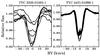 |
Fig. 1 CCFs for TYC 3226-01083-1 and TYC 4421-01996-1. Left panel: weak and highly variable CCF. Right panel: apparently unresolved spectroscopic binary. |
2.2. Atmospheric parameters
We adopted the atmospheric parameters for 327 stars from the paper by Zieliński et al. (2012). Stars with variable or weak CCF that were identified in the previous section were omitted for further analysis since their equivalent widths are very uncertain.
We also obtained atmospheric parameters for 13 stars (Table 1) from Zieliński et al. (2012), for which these authors only give rough estimates of stellar parameters, although our CCF analysis reveals a steady profile. We used ARES (Sousa et al. 2007) to measure equivalent widths (EWs) for neutral (Fe I) and ionized (Fe II) iron absorption lines from the line list of Takeda et al. (2005) as being the most suitable for our HET/HRS spectra (Adamów et al. 2015). Next, we used the resulting EWs to determine the atmospheric parameters with MOOG (Sneden 1973).
Furthermore, using an identical procedure to the one described in Zieliński et al. (2012), we obtained new atmospheric parameters for TYC 3011-00791-11, for which a better quality spectrum was available, and for TYC 4444-00200-1, which was misidentified by Zieliński et al. (2012; see Table 2).
The sample that we consider here contains 342 relatively bright field stars in total, mostly giants with Teff between 4055 K and 6239 K (G8-K2 spectral type), log g between 1.39 and 4.78, and the [Fe/H] between −1.0 to +0.45.
Updated stellar atmospheric parameters for 13 objects from red clump PTPS sample stars.
New stellar atmospheric parameters for two misidentified objects from red clump PTPS sample stars.
3. Construction of the probability distribution function
For the Bayesian analysis we adopted theoretical stellar models from Bressan et al. (2012) that were gathered from the interactive interface on Osservatorio Astronomico di Padova website2. We used isochrones with metallicity Z = 0.0001, 0.0004, 0.0008, 0.001, 0.002, 0.004, 0.006, 0.008, 0.01, 0.0152, 0.02, 0.025, 0.03, 0.04, 0.05, 0.06, and 0.008 interval in log (age/yr). The adopted solar distribution of heavy elements corresponds to the Sun’s metallicity: Z ≃ 0.0152 (Caffau et al. 2011). The helium abundance for a given metallicity was obtained from the relation Y = 0.2485 + 1.78 Z.
3.1. Mathematical formalism
We implemented the Bayesian method based on Jørgensen & Lindegren (2005) formalism and modified by da Silva et al. (2006) to avoid statistical biases and to take uncertainty estimates of observed quantities into consideration. For a given star, represented by full set of available atmospheric parameters (and its luminosity if the parallax was available): [ Fe/H ] ± σ[ Fe/H ], log Teff ± σlog Teff, log g ± σlog g, log L ± σlog L, isochrone of [Fe/H] and age t we calculated the probability of belonging to a given mass range.
The initial mass function for single star was taken from Salpeter (1955). Instead of an absolute magnitude like da Silva et al. (2006), we used the luminosity (if the parallax was available) and a logarithm of surface gravity. We further followed the procedure detailed in da Silva et al. (2006) and calculated searched quantities (e.g. mass, luminosity and age) and their uncertainties from basic parameters (mean, variance, etc.) of the normalised probability distribution functions (PDFs).
For stars with Hipparcos (van Leeuwen 2007) parallaxes, for which π>σπ, stellar luminosities were calculated directly and only stellar mass and age were obtained from PDFs.
3.2. Stellar radii
Using either stellar mass or luminosity derived from the Bayesian analysis and available atmospheric parameters, one can calculate stellar radii as either 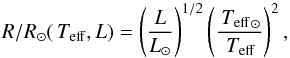 (1)or
(1)or  (2)where R⊙,M⊙,L⊙,Teff⊙ are solar values of radius, mass, luminosity, and effective temperature.
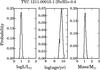 |
Fig. 2 Probability distribution functions for luminosity, mass, and age of TYC 1211-00015-1. |
4. Results
Typical examples of PDFs for luminosity, age, and mass – with an apparently unique set of solutions – are presented in Fig. 2. Compared with other parameters, the widest distribution and the lowest probability peak is present in the case of log (age/yr). As a consequence, the stellar ages obtained here are most uncertain. For 11 objects the PDF shows double peaks (see Fig. 3). For such stars we estimate two separate sets of solutions, the one with a higher value of PDF for stellar mass is listed first. The reason for this ambiguity is higher density (degeneracy) of stellar evolutionary tracks on the part of the Hertzsprung-Russell diagram that is occupied by many of our stars. The probability of obtaining non-unique and well-separated solutions is higher for red giant clump stars, that are common in our sample. The resulting stellar parameters with their uncertainties, are presented in Table 3.
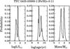 |
Fig. 3 Double peak probability distribution functions for luminosity, mass, and age of TYC 0435-03989-1. |
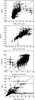 |
Fig. 4 Comparison of masses, luminosities, ages, and radii with their uncertainties from this work and with those from Zieliński et al. (2012). |
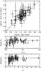 |
Fig. 5 Comparison of luminosities calculated from trigonometric parallaxes with our Bayesian estimates. |
The stellar masses that were obtained range from between 0.88 and 3.75 solar masses with the vast majority of stars (240 stars) having masses between 1.0 and 1.5 M⊙. The mean uncertainty in stellar mass is 0.19 M⊙. For log L/L⊙ we obtained values between 0.04 and 3.1, with 164 objects having luminosities between log L/L⊙ 1.5 and 2.0. For most of the stars, the uncertainty in log L/L⊙ is lower than 0.3. For 288 stars, with no trigonometric parallaxes, the mean uncertainty in log L/L⊙ is 0.13. Stellar ages, log (age/yr), range from 8.36 to 10.09 with mean uncertainty of ~0.18 dex.
The radii determined from Eq. (1) differ in most cases from those derived from Eq. (2) by more than the estimated uncertainties. In most cases (54%) the difference is lower than 10% of the mean value. For 80% of stars it stays within 30%, but uncertainties as high as 100% may occur. In Table 3 we present the mean values of radii derived from both equations and the total derivative as the estimate of the radius uncertainty. The resulting radii range from 1.32 to 50.24 solar radius, with the mean uncertainty of 3.16 solar radius.
4.1. Comparison with Zieliński et al. (2012)
For 288 objects without a trigonometric parallax, the available luminosities derived by Zieliński et al. (2012) agree very well with ours, with Pearsons correlation coefficient of r = 0.80. Our findings are, however, more precise. The estimated uncertainties are nearly two times lower than those of Zieliński et al. (2012). As a consequence, for these stars the radii calculated from Eq. (1) are also in good agreement. Our log (age/yr) determinations are in general larger by 0.15 dex, where r = 0.733.
Stellar masses obtained here, with an average value of 1.35 M⊙, are generally lower by over 0.1 M⊙ than those of Zieliński et al. (2012) – 1.5 M⊙, but at the same time the abundant population of stars with masses below solar is now absent. The resulting stellar masses are also more precise since the average uncertainty in Zieliński et al. (2012) is 0.28 M⊙. A comparison of stellar masses, as well as other parameters that were derived here with those of Zieliński et al. (2012), is presented in Fig. 4.
4.2. Comparison with other determinations
For eight stars our stellar masses can be compared with the findings of other authors. For HD 102272, BD+20 2457 and BD+48 740 we note good agreement with Mortier et al. (2013), well within 1σ of uncertainty. Out of five stars for which stellar masses were obtained by Sousa et al. (2015), all but one of ours have good agreement, within 1σ as well. The only exception is HD 240237, for which our new estimated stellar mass, 1.46 ± 0.32 M⊙, agrees within estimated uncertainties with those presented in Gettel et al. (2012) and Zieliński et al. (2012), while Sousa et al. (2015) found a mass of 0.614 ± 0.076 M⊙ for this star. We find their result rather uncertain as it is hard to believe that a star of that mass is already a giant with log g = 1.66 ± 0.15. Indeed, for the stellar mass of Sousa et al. (2015), the web interface for the Bayesian estimation of stellar parameters4 returns log g = 4.662 ± 0.358 for this object, which is contrary to the finding these authors present.
4.3. Comparison with luminosities from trigonometric parallaxes
For 54 objects with trigonometric parallaxes we compared our Bayesian luminosity estimates (using only log Teff, log g and [Fe/H], with their uncertainties as a stellar parameter input) with those calculated directly from trigonometric parallaxes (Fig. 5) and we found a relation log L/L⊙ ,π = (0.68 ± 0.11)log L/L⊙ + (0.72 ± 0.18) and the Pearson correlation coefficient of r = 0.66. As expected, the highest scatter is present for stars with the lowest parallaxes π< 5 mas. It is clear that the Gaia (Perryman et al. 2001) will provide parallaxes with high-level accuracy, which will allow better luminosities to be determined and, as a consequence, stellar masses for the stars presented here.
5. Conclusions
We presented stellar masses, luminosities and log (age/yr), obtained through a Bayesian analysis of atmospheric parameters available from Zieliński et al. (2012), as well as new estimates of radii for 342 stars, the targets of the PTPS. For 13 stars we present atmospheric parameters for the first time. For another two, we provide updated ones. The results, as based on a specific set of stellar evolutionary models, are obviously model-dependent. Based on the results of Thompson et al. (2014), we anticipate, however, that this introduces inaccuracy below estimated uncertainties in the mass range occupied by our targets.
As a consequence of the adopted stellar models our stellar masses take into consideration the mass-loss at the red giant branch but the resulting masses represent zero age main sequence masses for all stars. This obvious simplification is justified by the stellar mass range that we deal with in this project. A solar-mass star is not expected to lose more than 0.09 ± 0.03 M⊙ during its evolution up to the horizontal branch (Miglio et al. 2012), the effect of which contributes to only a small fraction of its estimated uncertainties.
As presented here, the stellar masses represent a significant improvement over previous findings because of the application of a much denser set of stellar models, and more detailed treatment of metallicities. As a result, a significant decrease in the uncertainty of stellar masses was achieved. An important result is also a thorough testing of an improved tool to derive stellar masses from available stellar atmospheric parameters in the PTPS sample.
The results for this star were already published in Niedzielski et al. (2015).
To compare with Zieliński et al. (2012) results for objects for which a range in log (age/yr) was presented, the maximum value of log (age/yr) from that paper was taken into consideration.
Acknowledgments
We acknowledge financial support from the Polish National Science Centre through grant 2012/07/B/ST9/04415. The Hobby-Eberly Telescope is a joint project of the University of Texas at Austin, the Pennsylvania State University, Stanford University, Ludwig-Maximilians-Universität München, and Georg-August-Universität Göttingen. The HET is named in honor of its principal benefactors, William P. Hobby and Robert E. Eberly.
References
- Adamów, M., Niedzielski, A., Villaver, E., Wolszczan, A., & Nowak, G. 2014, A&A, 569, A55 [NASA ADS] [CrossRef] [EDP Sciences] [Google Scholar]
- Adamów, M., Niedzielski, A., Villaver, E., et al. 2015, A&A, 581, A94 [NASA ADS] [CrossRef] [EDP Sciences] [Google Scholar]
- Bressan, A., Marigo, P., Girardi, L., et al. 2012, MNRAS, 427, 127 [NASA ADS] [CrossRef] [Google Scholar]
- Caffau, E., Ludwig, H.-G., Steffen, M., Freytag, B., & Bonifacio, P. 2011, Sol. Phys., 268, 255 [NASA ADS] [CrossRef] [Google Scholar]
- da Silva, L., Girardi, L., Pasquini, L., et al. 2006, A&A, 458, 609 [NASA ADS] [CrossRef] [EDP Sciences] [Google Scholar]
- Flannery, B. P., & Johnson, B. C. 1982, ApJ, 263, 166 [NASA ADS] [CrossRef] [Google Scholar]
- Gettel, S., Wolszczan, A., Niedzielski, A., et al. 2012, ApJ, 745, 28 [NASA ADS] [CrossRef] [Google Scholar]
- Girardi, L., Bressan, A., Bertelli, G., & Chiosi, C. 2000, A&AS, 141, 371 [NASA ADS] [CrossRef] [EDP Sciences] [Google Scholar]
- Jørgensen, B. R., & Lindegren, L. 2005, A&A, 436, 127 [NASA ADS] [CrossRef] [EDP Sciences] [Google Scholar]
- Mayor, M., & Queloz, D. 1995, Nature, 378, 355 [NASA ADS] [CrossRef] [Google Scholar]
- Miglio, A., Brogaard, K., Stello, D., et al. 2012, MNRAS, 419, 2077 [NASA ADS] [CrossRef] [Google Scholar]
- Mortier, A., Santos, N. C., Sousa, S. G., et al. 2013, A&A, 557, A70 [NASA ADS] [CrossRef] [EDP Sciences] [Google Scholar]
- Niedzielski, A., & Wolszczan, A. 2008, in IAU Symp. 249, eds. Y.-S. Sun, S. Ferraz-Mello, & J.-L. Zhou, 43 [Google Scholar]
- Niedzielski, A., Konacki, M., Wolszczan, A., et al. 2007, ApJ, 669, 1354 [NASA ADS] [CrossRef] [Google Scholar]
- Niedzielski, A., Wolszczan, A., Nowak, G., et al. 2015, ApJ, 803, 1 [Google Scholar]
- Nowak, G. 2012, Ph.D. Thesis, Nicolaus Copernicus University in Torun [Google Scholar]
- Nowak, G., Niedzielski, A., Wolszczan, A., Adamów, M., & Maciejewski, G. 2013, ApJ, 770, 53 [Google Scholar]
- Perryman, M. A. C., de Boer, K. S., Gilmore, G., et al. 2001, A&A, 369, 339 [NASA ADS] [CrossRef] [EDP Sciences] [Google Scholar]
- Ramsey, L. W., Adams, M. T., Barnes, T. G., et al. 1998, in Advanced Technology Optical/IR Telescopes VI, ed. L. M. Stepp, SPIE Conf. Ser., 3352, 34 [Google Scholar]
- Salpeter, E. E. 1955, ApJ, 121, 161 [Google Scholar]
- Shetrone, M., Cornell, M. E., Fowler, J. R., et al. 2007, PASP, 119, 556 [NASA ADS] [CrossRef] [Google Scholar]
- Sneden, C. A. 1973, Ph.D. Thesis, the university of Texas at Austin [Google Scholar]
- Sousa, S. G., Santos, N. C., Israelian, G., Mayor, M., & Monteiro, M. J. P. F. G. 2007, A&A, 469, 783 [NASA ADS] [CrossRef] [EDP Sciences] [Google Scholar]
- Sousa, S. G., Santos, N. C., Mortier, A., et al. 2015, A&A, 576, A94 [NASA ADS] [CrossRef] [EDP Sciences] [Google Scholar]
- Takeda, Y., Sato, B., Kambe, E., et al. 2005, PASJ, 57, 109 [Google Scholar]
- Thompson, B., Frinchaboy, P., Kinemuchi, K., Sarajedini, A., & Cohen, R. 2014, AJ, 148, 85 [NASA ADS] [CrossRef] [Google Scholar]
- Tull, R. G. 1998, in Optical Astronomical Instrumentation, ed. S. D’Odorico, SPIE Conf. Ser., 3355, 387 [Google Scholar]
- van Leeuwen, F. 2007, A&A, 474, 653 [NASA ADS] [CrossRef] [EDP Sciences] [Google Scholar]
- Zieliński, P., Niedzielski, A., Wolszczan, A., Adamów, M., & Nowak, G. 2012, A&A, 547, A91 [NASA ADS] [CrossRef] [EDP Sciences] [Google Scholar]
All Tables
Updated stellar atmospheric parameters for 13 objects from red clump PTPS sample stars.
New stellar atmospheric parameters for two misidentified objects from red clump PTPS sample stars.
All Figures
|
Fig. 1 CCFs for TYC 3226-01083-1 and TYC 4421-01996-1. Left panel: weak and highly variable CCF. Right panel: apparently unresolved spectroscopic binary. |
| In the text | |
|
Fig. 2 Probability distribution functions for luminosity, mass, and age of TYC 1211-00015-1. |
| In the text | |
|
Fig. 3 Double peak probability distribution functions for luminosity, mass, and age of TYC 0435-03989-1. |
| In the text | |
|
Fig. 4 Comparison of masses, luminosities, ages, and radii with their uncertainties from this work and with those from Zieliński et al. (2012). |
| In the text | |
|
Fig. 5 Comparison of luminosities calculated from trigonometric parallaxes with our Bayesian estimates. |
| In the text | |
Current usage metrics show cumulative count of Article Views (full-text article views including HTML views, PDF and ePub downloads, according to the available data) and Abstracts Views on Vision4Press platform.
Data correspond to usage on the plateform after 2015. The current usage metrics is available 48-96 hours after online publication and is updated daily on week days.
Initial download of the metrics may take a while.