| Issue |
A&A
Volume 586, February 2016
|
|
|---|---|---|
| Article Number | A38 | |
| Number of page(s) | 15 | |
| Section | Astrophysical processes | |
| DOI | https://doi.org/10.1051/0004-6361/201526630 | |
| Published online | 22 January 2016 | |
General relativistic magnetohydrodynamical simulations of the jet in M 87
1 Department of Astrophysics/IMAPP, Radboud University Nijmegen, PO Box 9010, 6500 GL Nijmegen, The Netherlands
e-mail: m.moscibrodzka@astro.ru.nl
2 ASTRON, Oude Hoogeveensedijk 4, 7991 PD Dwingeloo, The Netherlands
3 Department of Physics & Astronomy, The Johns Hopkins University, 3400 N. Charles Street, Baltimore, MD 21218, USA
Received: 29 May 2015
Accepted: 24 October 2015
Context. The connection between black hole, accretion disk, and radio jet can be constrained best by fitting models to observations of nearby low-luminosity galactic nuclei, in particular the well-studied sources Sgr A* and M 87. There has been considerable progress in modeling the central engine of active galactic nuclei by an accreting supermassive black hole coupled to a relativistic plasma jet. However, can a single model be applied to a range of black hole masses and accretion rates?
Aims. Here we want to compare the latest three-dimensional numerical model, originally developed for Sgr A* in the center of the Milky Way, to radio observations of the much more powerful and more massive black hole in M 87.
Methods. We postprocess three-dimensional GRMHD models of a jet-producing radiatively inefficient accretion flow around a spinning black hole using relativistic radiative transfer and ray-tracing to produce model spectra and images. As a key new ingredient in these models, we allow the proton-electron coupling in these simulations depend on the magnetic properties of the plasma.
Results. We find that the radio emission in M 87 is described well by a combination of a two-temperature accretion flow and a hot single-temperature jet. Most of the radio emission in our simulations comes from the jet sheath. The model fits the basic observed characteristics of the M 87 radio core: it is “edge-brightened”, starts subluminally, has a flat spectrum, and increases in size with wavelength. The best fit model has a mass-accretion rate of Ṁ ~ 9 × 10⁻³M⊙ yr-1 and a total jet power of Pj ~ 1043 erg s-1. Emission at λ = 1.3 mm is produced by the counter-jet close to the event horizon. Its characteristic crescent shape surrounding the black hole shadow could be resolved by future millimeter-wave VLBI experiments.
Conclusions. The model was successfully derived from one for the supermassive black hole in the center of the Milky Way by appropriately scaling mass and accretion rate. This suggests the possibility that this model could also apply to a wider range of low-luminosity black holes.
Key words: accretion, accretion disks / black hole physics / relativistic processes / galaxies: jets / galaxies: nuclei
© ESO, 2016
1. Introduction
The most notable signature of an active black hole (BH) is a radio jet, but the exact processes of jet production by an accretion disk around a spinning BH, as well as its collimation and acceleration, has not been fully established. The radio core in the center of the Milky Way (hereafter Sgr A*) and in the center of the massive elliptical galaxy M 87 – two sources that can be observed with unprecedented resolution – display nearly flat radio spectra that are characteristic of relativistic jets (Blandford & Königl 1979; Falcke & Biermann 1995). For both objects, the combination of the putative central BH mass (MBH) and distance (D) provide an expected angular size of the BH on the sky ( and 38 μas, for Sgr A* and M 87, respectively). In principle, therefore, they can be resolved (together with the surrounding plasma) with current radio and millimeter very long baseline interferometers (VLBI). Millimeter-VLBI observations promise to provide essential clues about the jet-disk-BH connection because they will probe plasma in the immediate vicinity of a BH in these two sources. Since Sgr A*’s intrinsic geometry is smeared out by an interstellar scattering screen (e.g., Bower et al. 2014), the nature of the radio emission near the central supermassive black hole (SMBH) remains hidden, so it is somewhat difficult to probe its putative jet intrinsic geometry and properties. On the other hand, the radio core of M 87 is resolved into a clear jet structure and can be readily used as a laboratory for testing various theoretical models of the magnetized plasma flows onto compact objects.
The M 87 core is a prototype of a radio loud low-luminosity active galactic nuclei (Ho 2008, and references therein). The bolometric luminosity of the core is estimated to be L/LEdd ≈ 10-7, which suggests that the powerful (the jet power is Pj ≈ 1045 erg s-1, de Gasperin et al. 2012) kpc-scale jet emerges from a radiatively inefficient accretion flow (RIAF) onto the supermassive BH (Yuan & Narayan 2014). A similar, downsized model is often used to explain the L/LEdd ≈ 10-9 emission from Sgr A*. In fact, radio cores seem to be rather ubiquitous in low-luminosity AGN (LLAGN; Nagar et al. 2000) and scale with mass and accretion rate in a simple way (Merloni et al. 2003; Körding et al. 2006). One would therefore expect a generic RIAF+jet model to equally scale between AGN of different masses and accretion rates.
Advances in the field of numerical astrophysics now allows magnetized RIAFs and their jets to be simulated almost from the first principles (e.g., Abramowicz & Fragile 2013; Yuan & Narayan 2014; and references therein). General relativistic radiative transfer (GRRT) models can predict the general relativistic magnetohydrodynamical (GRMHD) simulation spectrum and appearance. This allows us to compare dynamical models directly to VLBI observations (e.g., Dexter et al. 2012; Hilburn & Liang 2012; Mościbrodzka et al. 2014).
However, a few crucial uncertainties in the GRMHD simulations and GR radiative transfer simulations do not yet allow one to tightly constrain these models and to closely examine whether the BH spin or the magnetic fields play the most critical role in jet formation. One of the main uncertainties in GRMHD simulation is associated with the distribution function (DF) of radiating particles (electrons). Electron DF is not explicitly computed in any of the current GRMHD simulations. Moreover, as shown in Mościbrodzka et al. (2014), the appearance of a GRMHD model strongly depends on the details of the assumed electron temperature (the so-called “painting” of GRMHD simulations). Moreover, the true electron DF in the magnetized plasma can vary with space and time, which leaves us many degrees of freedom in the interpretations of observational data.
Recently, we have phenomenologically found a simplified but natural, location-dependent prescription for electron DFs in the GRMHD models that is able to reproduce observational characteristics of Sgr A* (Mościbrodzka & Falcke 2013; Mościbrodzka et al. 2014). In particular, the flat spectrum of the source can be reproduced when we assume that electrons along the jet funnel (i.e., in the jet sheath) produced by the RIAF are hotter than those in the RIAF (accretion disk) itself. In this electron model, we assumed that electrons in the accretion disk have a thermal, Maxwellian distribution function, but they are weakly coupled to protons, so the plasma is two-temperature in the disk, and electrons are rather cool. At the same time, to account for radio emission of Sgr A*, we assumed that the electrons in the jet and in the jet wall are much hotter than in the accretion disk. Under this assumption, the strongly magnetized jet becomes brighter than the relatively weakly magnetized disk in radio wavelengths. In other words, the model appears to the observers as a jet-dominated advective system (JDAF).
We have also found that the emission from the tenuous jet wall in the simulations can account for the entire radio spectrum of Sgr A* (when the jet extends by 2−3 orders of magnitude in radius) and the two-temperature disk is visible around millimeter wavelengths and shorter. The jet images were edge-brightened in a similar way because it is observed in the M 87 jet (e.g., Ly et al. 2007). The next logical step is thus to scale the same model to M 87 to test if the model can reproduce the radio observations of the M 87 jet. Furthermore, the M 87 core is also a target of the Event Horizon Telescope (EHT, Doeleman et al. 2012), which is a millimeter Very Long Baseline Interferometric experiment to image the central BH and its surrounding in Sgr A* and M 87. It is natural to ask whether the BH illuminated by the footprint of a relativistic jet is detectable by the EHT (Dexter et al. 2012).
The goal of this work is to examine how the footprint of the jet would appear in radio observations and to study how the apparent size of the jet depends on wavelength. Ultimately, the model should be constrained by the multi-wavelength VLBI data at 7 mm, 3.5 mm, and 1.3 mm, which is already available. In this work, we use the same three-dimensional (3D) GRMHD model that was used by us to model Sgr A* (Mościbrodzka et al. 2014), but rescaled to the mass of the BH in M 87.
The paper is organized as follows. In Sect. 2, we briefly present the 3D GRMHD model and radiative transfer technique and describe how we scale the model to the M 87 system. We also introduce some of the observational constraints used in our models. In Sect. 3, we compare the model spectra and radio images directly to λ = 7, 3.5, and 1.3 mm observations of the inner jet in M 87. We discuss our results in the context of results found in the literature in Sect. 4. We conclude in Sect. 5.
2. Models of a jet
2.1. Dynamics of plasma and magnetic fields
Our time-dependent model of a radiatively inefficient accretion flow onto a BH is based on the fully, three-dimensional (3D) GRMHD simulation carried out by Shiokawa (2013) (run b0-high in Table 5.1 in Shiokawa 2013). The simulation started from a torus in hydrodynamic equilibrium in the equatorial orbit around a rotating BH (Fishbone & Moncrief 1976). The torus initially had a pressure maximum at 24 GMBH/c2 and an inner edge at 12 GMBH/c2. It was seeded with a weak poloidal field that follows the isodensity contours (single-loop model, see Gammie et al. 2003). The dimensionless BH spin was a∗ ≃ 0.94. The corresponding radius of the event horizon was rh = 1.348 GMBH/c2 and the innermost stable circular orbit (ISCO) was located at rISCO = 2.044 GMBH/c2. The inner boundary of the computational domain was just inside the event horizon and the outer boundary was at Rout = 240 GMBH/c2. The model was evolved for 14 000 GMBH/c3, which is equivalent to about 19 orbital periods at r = 24 GMBH/c2.
Jets are naturally produced in the GRMHD simulation and are defined as the strongly magnetized and nearly empty regions above the BH poles. We refer to this region as the jet spine. Close to the BH, most of the energy of the jet spine is stored in the magnetic fields that cannot be radiated away efficiently. Although it is uncertain, the plasma density in the jet spine is most likely very low; as a result, this region would not produce any significant radio or synchrotron emission (see, e.g., Mościbrodzka et al. 2011). However, as noted by Mościbrodzka & Falcke (2013) and Mościbrodzka et al. (2014), the jet definition should also include the jet sheath, which is a tenuous layer of gas that moves along the jet spine. The jet sheath is less magnetized in comparison to the spine (the plasma β parameter decreases with radius from 50 to 1 in the jet sheath, while β ≲ 1 in the spine), but has higher matter content that can be constantly resupplied by an accretion disk.
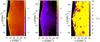 |
Fig. 1 Dimensionless electron temperature, Θe = kTe/mec2, in the model with Rhigh = 1 (left panel) and Rhigh = 100 (middle panel). The right panel shows the proton-to-electron temperature ratio in the model with Rhigh = 100. The maps show the slices through the 3D GRMHD model (run b0-high in Table 5.1 in Shiokawa 2013) along the BH spin axis. |
2.2. Emission model
The radiative properties of the dynamical model are studied by post-processing the GRMHD model with radiative transfer (RT) computations. Calculations are carried out using the same tools as in Mościbrodzka et al. (2009). The spectral energy distributions (SEDs) are computed using a Monte Carlo code for relativistic radiative transfer grmonty (Dolence et al. 2009) that includes radiative processes, such as synchrotron emission, self-absorption, and inverse-Compton processes. To create model images, a ray-tracing radiative transfer scheme is used (Noble et al. 2007). Both RT schemes solve RT equations for total (unpolarized) intensity along null-geodesics trajectories.
Local plasma synchrotron emissivity (jν) and absorptivity (αν) depend on the assumed electron distribution function, the angle between magnetic field and the plasma velocity vectors, the magnetic field strength, and the electron number density. The resulting spectrum detected by an observer will therefore depend on the observer’s orientation with respect to the synchrotron source, structure, and bulk speed of plasma and magnetic field geometries. Near a BH, the emission is also affected by spacetime curvature. In our models, we take all these effects into account; i.e., the radiative transfer code includes all the variables mentioned earlier, except the electron distribution function (see next section), directly from the GRMHD accretion flow model.
2.3. Electron DF in the disk and in jets
It is almost certain that electron DFs are non-thermal, power-law functions, but for simplicity, in our modeling, electrons are described by a Maxwell-Jüttner distribution parameterized by Θe = kTe/mec2. While the proton temperature Tp is provided by the GRMHD simulation, we assume that the electron temperature Te depends on plasma magnetization. The electron temperature is calculated from the following formula:  (1)where b = β/βcrit, β = Pgas/Pmag, and Pmag = B2/ 2. We assume that βcrit = 1, and Rhigh and Rlow are temperature ratios that describe the electron-to-proton coupling in the weakly magnetized (disk, high β regions) and strongly magnetized regions (jet, low β regions), respectively. In Eq. (1), the proton-to-electron temperature ratio scales with β2, which guarantees that the regions of strong and weak proton-to-electron coupling are clearly defined, and their radiations are easy to distinguish and to interpret, which would not be the case if the temperature ratio scaled linearly with β. In our RT model, the accurate synchrotron emissivities for thermal, relativistic electrons are adopted from Leung et al. (2011).
Our new electron temperature definition (Eq. (1)), which describes the electron temperatures in the jet and disk zones, has been slightly modified compared to the one used in Mościbrodzka et al. 2014, (in which we defined the jet zones as unbound plasma, and electrons in the jet had constant temperature). This is done to avoid artifacts such as sharp boundaries between the disk and jet zones. Nevertheless, the current model is similar to the one in Mościbrodzka et al. (2014), where the accretion disk and the jets are described as a two-temperature and a single-temperature plasma, respectively. Here, we simply associate the plasma temperatures with plasma magnetization, which is physically more intuitive.
We consider six models with fixed Rlow = 1 and varying Rhigh = 1,5,10,20,40,100. In Figs. 1 and 2, we show maps of electron temperature calculated using Eq. (1) for two extreme cases (Rhigh = 1 and 100) and the proton-to-electron temperature ratio when Rhigh = 100. The electron temperature is expressed in units of electron rest mass, Θe = kTe/mec2, and Θe ≳ 0.1 for plasma to emit synchrotron radiation. In models with Rhigh = 100, the plasma with temperatures Θe> 1 occupies the tenuous jet wall (see Fig. 1, right panel).
For fixed Rlow = 1 and Rhigh> 100, the electron temperature in the jet wall becomes sub-relativistic and does not produce any continuum synchrotron emission. Values of Rlow that are less than unity are also physically possible when electrons are additionally heated up, such as in magnetic field reconnection events or by turbulence. Our models assume ideal-MHD conditions, and turbulence in the tenous jet wall is unresolved. For the self-consistency of models, we do not consider models with Rlow< 1.
Summary of the radiative transfer models.
2.4. Scaling the model to M 87 core
The core and jet of M 87 have been observed mostly in radio but also in optical and X-ray bands. An excellent overview of M 87 jet properties and a list of references to the source observations is given in Biretta & Junor (1995) and more recently in Nakamura & Asada (2013).
To scale the dimensionless GRMHD simulation to astrophysical sources, one has to provide the central BH mass, its distance to the observer, and the mass of the accretion disk around the BH (which is equivalent to changing the mass accretion rate onto the SMBH). Based on the stellar or gas dynamics in the core, the mass of the M 87 central BH has been estimated as MBH = 3.2,3.5, and 6.2 × 10⁹M⊙ (by Macchetto et al. 1997; Gebhardt et al. 2011; Walsh et al. 2013, respectively). Here, we adopt the most recent value from the observations, MBH = 6.2 × 10⁹M⊙, in all of our models. The distance to M 87 is assumed to be the same as the mean distance to the Virgo cluster: D = 16.7 Mpc (Mei et al. 2007).
The BH mass MBH sets the length unit (the gravitational radius) GMBH/c2 = 9.2 × 1014 cm = 2.89 × 10⁻⁴ pc and sets the model time unit to be GMBH/c3 = 8.5 h. The GRMHD snapshots used in the radiative transfer modeling were evolved for 10 000 GMBH/c3 time units, which corresponds to approximately 10 yr. We analyzed the GRMHD simulation time slices for a short time interval of about 1000 GMBH/c3 ≡ 350 d dumped by the code every 10 GMBH/c3 ≡ 3.5 d. The GRMHD model diameter of 480 GMBH/c2 corresponds to about 1.8 mas on the sky for the chosen MBH and D.
The orientation of the source with respect to the observer is described by two angles: inclination angle, i, and position angle, PA. These can be estimated from the observations of the M 87 jet at radio and optical wavelengths. However, we simply assume two inclination (viewing) angles, i = 20 and 160°. At the viewing angle of 160°, the model rotates in the opposite direction to i = 20°. The direction of the rotation of the system is also examined. In the models presented in this paper, we adopted the position angle of the BH spin on the sky as PA = 290°, estimated from radio observations by Reid et al. (1982).
The mass accretion rate onto the SMBH, Ṁ, is a free parameter. The accretion rate can be estimated by fitting the model SED to the multiwavelength observational data points.
The X-ray luminosity of the central region (<2′′) around the BH is estimated as 4−7 × 1040 erg s-1 (Marshall et al. 2002; Di Matteo et al. 2003). The radio spectrum is nearly flat with the flux FR ~ 1 Jy. Our SED models, computed for a range of Rhigh values, are normalized such that the flux at λ = 1.3 mm is 1 Jy (see Doeleman et al. 2012). The normalization can be achieved by adjusting Ṁ. In the models presented in this work, Ṁ ranges from 10-4 to 10-2M⊙ yr-1, and Rhigh from 1 to 100.
The mass accretion rate in the model is changed by multiplying the plasma density by a constant number. The magnetic field strength in the model is described by a dimensionless plasma parameter β, therefore by changing the model density normalization, we automatically change the strength of the magnetic field in the entire model ( ). The observational constraint on the accretion rate can also be inferred from the observed Faraday rotation at λ = 1.3 mm, and RM = ± a few × 105 rad m-2 (Kuo et al. 2014). However, the Ṁ derived based on RM is strongly model dependent. We calculate RM self-consistently based directly on the GRMHD and RT models (see Sect. 4.1).
 |
Fig. 3 Electromagnetic spectrum of GRMHD models computed at i = 20° and i = 90° based on models RH1-RH100 overplotted with the observations of M 87 collected in Abdo et al. (2009). Synchrotron emission appears in the SED as a hump around 230 GHz, and the higher order humps (second and third ones) are due to inverse-Compton emission. |
 |
Fig. 4 Intensity map of our fiducial model RH100 at λ = 7 mm (ν = 43 GHz) for a viewing angle of i = 20° (left panel) and i = 160° (right panel). The color scale is normalized to unity. See Table 1 for the total fluxes in units of Jansky for each model (Col. 7). The position angle of the jet axis/black hole spin is set to PA = 290° (Reid et al. 1982) E of N for both models. The size of each panel is 200 × 200 GMBH/c2 in the plane of the black hole. At a distance of D = 16.7 Mpc, this corresponds to an angular size of about 0.8 × 0.8 mas. |
3. Results
3.1. Modeling radiative efficiency and SEDs data
Here, we present model spectra for six different combinations of Rhigh and Rlow (in Eq. (1)). Table 1 summarized the parameters used in these models. Figure 3 shows SEDs of models RH1-RH100 for i = 20° and for i = 90°. The SEDs for i = 90° are given as reference to demonstrate that most of the higher (than 230 GHz) energy radiation is emitted from the system in the direction (along the equatorial plane) away from our fixed line of sight. The numerical code includes radiative processes, such as the synchrotron emission and self-absorption, which appears in the SED as a hump around (230 GHz) and the inverse-Compton scatterings (higher order humps).
Another important process is bremsstrahlung from electron-proton and relativistic electron-electron collisions. We have implemented bremsstrahlung in our radiative transfer code (details presented in Appendix D of Mościbrodzka et al. 2011). Our calculations of bremsstrahlung emission from all presented 3D models indicate that the majority of the bremsstrahlung radiation is produced in the accretion disk regions at radii r> 24 GMBH/c2 (beyond the pressure maximum of the initial torus configuration). However, we note that the accretion disk structure and dynamics at r> 24 GMBH/c2 are simply artifacts of the adopted initial plasma configuration (the torus). This makes any bremsstrahlung emission highly uncertain and therefore omitted in the current work. Bremsstrahlung emitted from within 24 GMBH/c2 is negligible compared to the inverse-Compton emission.
In Fig. 3, we also plot the observational data points from Abdo et al. (2009) and Doeleman et al. (2012). As already mentioned, our models are normalized to reproduce the flux of 1 Jy at 1.3 mm (230 GHz). In Fig. 3, the angular resolution of Fermi (data points at E> 100 MeV, or 1022 Hz) is large ( ), and data points include flux from the entire jet including its radio lobes (e.g., include HST-1 and other knots located further downstream of the jet, which are prime locations for the particle acceleration, hence the high-energy emission). Therefore the high-energy spectrum is used in this work as an upper limit. The proton-to-electron temperature ratio in the accretion disk has to be Rhigh ≥ 100 to produce a flux of 1 Jy at 1.3 mm, but not to overpredict the source luminosity measured at high energies.
In the rest of the paper, we therefore focus on modeling images of the fiducial model RH100 whose SED agrees with the observational data points. The radiative efficiencies for all models and the importance of the radiative cooling is discussed in Sect. 4.2. The radio maps’ appearance as a function of Rhigh is presented and briefly discussed in the Appendix.
 |
Fig. 5 Evolution of the intensity profile across (left panel) and along (right panel) the jet at λ = 7 mm (ν = 43 GHz). Color lines represent intensity at various times spaced by 20M ≡ 7 days. |
 |
Fig. 6 Contour maps of the model images (RH100) at λ = 7 mm (ν = 43 GHz) for viewing angles of i = 20° (left panel) and i = 160° (right panel) convolved with the telescope beam to simulate observations by Hada et al. (2011). The contour levels were chosen to match those from observations (contours decrease by a factor of 21 / 2 from the maximum intensity). The image size here is 480 × 480GMBH/c2 ≡ 1.8 × 1.8 mas, which is about twice the size used in Fig. 4 (images at λ = 7 mm). |
3.2. Emission at λ = 7 mm and 3.5 mm
Figure 4 shows the appearance of our fiducial model RH100 at λ = 7 mm for i = 20° (left panel) and i = 160° (right panel). The images show the intensity distributions on the sky that are normalized to unity. They are computed on the GRMHD model snapshot base and then time-averaged over a duration of about 35 d. At 7 mm, the plasma around the maximum of the intensity distribution is optically thick (the synchrotron photosphere, τabs = 1 surface, is located at a distance of about 10−25 GMBH/c2 from the BH). The images display extended and complex structures that are evidently edge-brightened. Moreover, there is the brightness asymmetry between the two rims on both sides of the jet. The jet is corotating with the BH and the disk. (The angular momentum vector of the BH, and the disk is pointing in the N-W direction in the images.) The brightness assymetry is due to Doppler boosting. In both cases shown in Fig. 4, the emission from the counter-jet is strongly suppressed.
 |
Fig. 7 Same as Fig. 4 but for λ = 3.5 mm (ν = 86 GHz). Here the panel size is 100 × 100GMBH/c2 in the plane of the black hole, which corresponds to an angular size of about 480 × 480 μas. |
The edge-brightening of the jet images is illustrated in Fig. 5 (left panel), which shows the radiation intensity profile across the jet axis at a distance of 25GMBH/c2 away from the SMBH. Figure 5 (left panel) shows how the intensity profile evolves in time. Lines with different colors indicate the intensity profile at various times. The time span between the black and magenta lines corresponds to about 28 d. The ratio of the intensity of the two rims is about two and is roughly constant in time. Figure 5 (right panel) also shows the evolution of intensity profile along the jet. The profile along the jet shows two intensity enhancements that apparently move upstream of the jet (“knots” located at x ~ 45 and 65GMBH/c2). We find that these two intensity “knots” have subluminal apparent speeds of v/c = 0.13 and 0.4, which indicate jet acceleration.
A robust comparison of Fig. 4 to observations of the source at 7 mm is presented in Hada et al. (2011). In Fig. 6, we convolve our theoretical intensity maps (Fig. 4) with the telescope beam size (FWHMbeam = 0.3 and 0.14 mas, see Hada et al. 2011) and contour them in the same fashion as Fig. 3b in Hada et al. (2011). There is overall good qualitative agreement, but also some remaining differences. Our jet model is somewhat more compact in the direction along the jet axis to account for the extended low-surface brightness jet features observed at 7 mm. Also our jet model does not display the characteristic two rims when convolved with the telescope beam, even though the underlying theoretical model is clearly edge-brightened. An even better agreement between our model and observations could probably be achieved (1) by using GRMHD models with a higher spatial resolution that resolves the jet boundary better; (2) by increasing the size of the computational domain since we are only simulating the innermost parts of the jet at 43 GHz; and (3) by including particle acceleration mechanisms, i.e., power laws in electron DFs, which are omitted here for the sake of simplicity. Adding a power law to the thermal energy distribution will amplify the optical part of the emission, hence also enhance the extended jet emission, which is optically thin after all.
Figure 7 shows two models’ (i = 20° and 160°) images at 3.5 mm. The emission from the jet has a parabolic shape (consistent with Hada et al. 2011), and it is edge-brightened as in the 7 mm images (Fig. 4). The emission from the counter-jet is more pronounced compared to the 7 mm images. However, owing to lensing effects, the counter-jet images resemble a disk structure. Overall, the emission becomes more compact at λ = 3.5 mm compared to the one in the 7 mm image, indicating the well-known λ dependency of the apparent sizes.
3.3. Emission near the BH horizon at λ = 1.3 mm
In Fig. 8 the lefthand panels display 1.3 mm images of model RH100 for i = 20° and i = 160°. At 1.3 mm the images are dominated by the emission from the counter-jet, while the emission from the jet on the near side (the one approaching the observer) is notably weaker. The emission is produced near the jet launching point and is compact. The emission around the BH has a shape of a crescent, which is simply a lensed image of the counter-jet1. However, the approaching-jet appears as an additional circle in front of the crescent. For our adopted position angle of the BH spin (PA = 290°; Reid et al. 1982), the emitting region is elongated in the E-W direction on the sky. In both images the BH shadow size is about 40 μas, as expected.
The core of M 87 has been detected at 1.3 mm with VLBI (Doeleman et al. 2012). The reconstruction of a 1.3 mm radio map using these observations was not possible because of an insufficient number of mm-VLBI stations. In this section, the comparison of 1.3 mm emission maps and the observations will be done in terms of interferometric observables.
 |
Fig. 8 Intensity maps of model RH100 for i = 20° (upper left panel) and i = 160° (lower left panel) at λ = 1.3 mm (ν = 230 GHz). The total fluxes (at 1.3 mm) in these models are 1 Jansky. The position angle of the black hole spin is set to PA = 290° E of N for all models. The image size is 40 × 40 GMBH/c2 in the plane of the black hole, which at a distance of D = 16.7 Mpc, corresponds to an angular size of about 140 × 140 μas. Middle panels: the corresponding visibility amplitude on a u−v plane in units of Jy. Right panels: the visibility phase map in degrees. The arrows in the left and middle panels indicate the orientation of our coordinate system. |
The interferometric observables are the visibility amplitude and phase as a function of u−v coordinates (distances between pairs of millimeter telescopes or spacial frequencies). The complex visibility function that an interferometer “detects” (Fourier transformation of the intensity distribution on the sky) is defined as follows 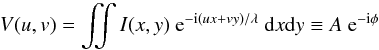 (2)where I(x,y) is the intensity distribution at a given set of lefthanded coordinates on the sky (i.e., x and y are positive in E and N directions on the sky, respectively), and u,v are the projected lefthanded baseline lengths (i.e., u and v are positive in eastern and northern directions on the Earth, respectively). Our intensity distributions based on GRMHD models are strongly non-Gaussian and so V(u,v) is a complex function that has non-trivial amplitude, A, and a non-zero phase, φ. In Fig. 8 the middle and righthand panels show the complex visibility amplitude and phase of the 1.3 mm intensity maps (displayed in the left panels), respectively.
In the middle panel of Fig. 8, the visibility amplitude maps show two minima for baselines with sizes 5000−6500 Gλ, which correspond to the angular size of the BH shadow. Figure 9 shows a cut of the visibility amplitude along E-W and N-S baselines. Evidently, along E-W baselines, the model displays two minima (at baselines of about about 4000−5000 and 10 000−8000 Mλ, where Mλ = 1.3 km) for both inclinations. Along N-S oriented interferometric baselines, there are no visible minima.
The core emission of M 87 has been detected at 1.3 mm on VLBI baselines between the Arizona Radio Observatory’s Submillimeter Telescope (SMT), the Combined Array for Research in Millimeter-wave Astronomy (CARMA), and the James Clerk Maxwell Telescope in Hawaii (Doeleman et al. 2012). The baselines of the telescope pairs are on the order of 800, 3500, and 4300 km (or equivalently 620, 2600, and 3300 Mλ). In Fig. 10, we make a crude comparison of our model visibility amplitudes to those observed by the EHT to test whether model RM100 is roughly consistent with the data for both inclination angles (i = 20° and 160°).
The visibility phase and, in particular, the so-called closure phase, which contains information on the source structure, can also constrain the model. The closure phase is the sum of visibility phases for a triangle of interferometric baselines:  (3)For a symmetrical Gaussian intensity distributions on the sky, the visibility phase is expected to be zero and so is the closure phase. Any deviation from a zero closure phase will indicate the source deviation from a Gaussian or point-like structure, and this observable can in principle be used to compare the model and observed emission shape without reconstructing the radio maps.
We have calculated the theoretical visibility closure phases. For the model with i = 20°, which shows the crescent on the N side of the BH (see Fig. 8), the closure phases are positive; φclosure = 11°,19°,11°,11°, where the four values correspond to different time moments of the observation. The φclosure evolution is caused by the rotation of the Earth, and it is probing slightly different u−v values. A typical observation duration is two to three hours. This is about three times shorter than the dynamical time scale of the source (8.5 h) with its BH mass, 6.2 × 10⁹M⊙. For i = 160°, for which the crescent is on the S side of the BH (Fig. 8), the closure phases are negative: φclosure = −21°, − 21°, − 12°, − 9.5°. In both cases, the values are consistent with the observed value: φclosure ≈ ± 20° (Akiyama, priv. comm.).
In summary, for the fiducial model RH100 (for both viewing angles of i = 20° and 160°), visibility amplitudes and closure phases are roughly consistent with the preliminary observations of the M 87 core obtained by the EHT (visibility amplitudes and closure phases on a single VLBI triangle).
 |
Fig. 9 Theoretical visibility amplitudes along E-W (left) and N-S (right) baselines, computed for model RH100 with i = 20°(solid lines) and 160°(dashed lines). |
4. Discussions
Deriving the appearance of a jet in the direct vicinity of a SMBH is not straightforward. The jet formation mechanism, as well as particle acceleration in jets, is generally not understood well. Moreover, one has to take spacetime curvature into account, which affects the plasma dynamics and light propagation. Using GRMHD simulations of a weakly magnetized accretion flow, a jet appears naturally, and we calculate the appearance of the M 87 jet base at radio and millimeter wavelengths. For the electron heating, we assume that the electrons are weakly coupled to protons in the accretion disk and strongly coupled in the jet – a simple, but crucial concept that we have already used successfully to explain the appearance of the SMBH in the center of the Milky Way. Below we discuss our results in a context of observational constraints. We also discuss the model limitations.
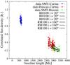 |
Fig. 10 Comparisons of the visibility amplitudes from our models and those from the EHT observations. The visibility amplitudes, computed at λ = 1.3 mm (ν = 230 GHz), along three baselines (SMT-CARMA, SMT-HAWAII, and CARMA-HAWAII) are shown for model RH100 with i = 20°(solid lines) and 160° (dashed lines). The distance between the VLBI stations is expressed in units of Mλ (1Mλ ≡ 1.3 km). The observed visibility amplitudes (points) and the u−v tracks are taken from Doeleman et al. (2012). |
4.1. Mass-accretion rate
The accretion rate onto M 87 is estimated by fitting the GRMHD model SED to the observed data points. The resulting best fit Ṁ will vary depending upon the underlying electron distribution functions in the accretion disk and jet. They typically vary between Ṁ = 10-4−10-2M⊙ yr-1 (Mościbrodzka et al. 2011, Hilburn & Liang 2012, Dexter et al. 2012). In our fiducial model RH100, we find Ṁ = 9 × 10⁻³M⊙ yr-1.
The mass-accretion rate can be also inferred from the observed Faraday rotation (e.g., at 1.3 mm). For example, Kuo et al. (2014) measured RM = ± afew × 105 rad m-2. They claim that this RM puts an upper limit on the accretion rate of Ṁmax ≈ 10-3M⊙ yr-1. However, the Ṁ derived from RM is strongly model dependent. We therefore directly calculate the RM from our GRMHD models to test whether our model agrees with the observed value by Kuo et al. (2014). The Faraday rotation measure is defined as  (4)where Θe, ne, and B|| are the dimensionless plasma electron temperature, density, and magnetic field component projected along the null geodesics. For a relativistically hot plasma, the correction term in Eq. (4) becomes
  . Density and field strength in Eq. (4) are given in c.g.s. units.
The integration of RM is performed along the null geodesics from the observer to the τλ = 1.3 mm = 1 surface. The synchrotron photosphere at 1.3 mm is located near the event horizon, where the emission contribution is mainly from the counter-jet. For models RH1-RH100, the time-averaged and intensity-weighted RM are 4 × 103,8 × 104,−7 × 10⁵,−6 × 10⁶,−6 × 10⁸, and−1 × 10¹⁰ rad m-2, respectively. As a result, model RH10 matches the observational RM best. Consequently, the mass-accretion rate of model RM10 is also similar to the value estimate in Kuo et al. (2014). The RM in model RH100 is too large. However, it is important to realize that the Faraday rotation measured in our simulation is certainly overestimated and somewhat meaningless because of the initial conditions of the torus (see, e.g., the density profile in the accretion disk in Fig. 2 top left panel in Mościbrodzka et al. 2014). This setup was chosen to provide a large mass reservoir from which the SMBH is fed on small scales without the need for a continuous mass flow from the outer boundary.
A reliable RM can therefore not be derived from our model, but requires simulations that self-consistently feed the BH on large scales. While this is computationally very expensive, this will be important to check in the future.
4.2. Importance of radiative cooling
Our GRMHD simulation is decoupled from radiative transfer calculations. To test that the radiation affects the dynamics of plasma in the simulation, we first examine the radiative efficiency of our models. The radiative efficiency can be measured with a simplified formula: ϵr = LBol/Ṁc2, where Ṁ is the time-averaged mass accretion rate computed at the event horizon of the BH. The ϵr are presented in Table 1 (sixth column). One would hope that ϵr< 1, however, for most of the models (RH1-RH20) ϵr> 1. These apparently too high radiative efficiencies are unphysical and indicate either that models with RH1-RH20 are self-inconsistent or that the method of computing the radiative efficiency is oversimplified. The high luminosities could be produced by a few localized places in the flow that contribute to the total luminosity significantly, which might not be reflected in the time-averaged mass accretion rate at the event horizon. We can either discard the self-inconsistent models or propose more accurate ways of measuring radiative efficiency of the accretion flow.
A more appropriate and accurate test for the importance of the radiative losses is to compute the radiative cooling timescale τrad = u/ Λ, where u is the specific energy density of gas and Λ the cooling rate, and compare it to the local dynamical timescale,  . The basic radiative process is synchrotron cooling, Λsyn. Following Mościbrodzka et al. (2011), we use
 ![\begin{equation} \Lambda_{\mathrm{syn}}= \frac{4 e^4 }{3 c^3 m_{\rm e}^2 } n_{\rm e} B^2 \left[\Theta_{\mathrm{e}}^{4/3} + (2\Theta_{\mathrm{e}})^{8/3}\right]^{3/4} \, \, {\rm erg\,cm}^{-3} \, {\rm s}^{-1}. \end{equation}](/articles/aa/full_html/2016/02/aa26630-15/aa26630-15-eq175.png) (5)We notice that Λsyn should be reduced to account for the synchrotron self-absorption and should be increased to account for the cooling in the inverse-Compton process. The current Λsyn is a crude approximation of the real cooling function, which might be a few times larger.
(5)We notice that Λsyn should be reduced to account for the synchrotron self-absorption and should be increased to account for the cooling in the inverse-Compton process. The current Λsyn is a crude approximation of the real cooling function, which might be a few times larger.
Here we only use the simplified formula. Mimicking full RT (coupling GRMHD with GRRT is beyond the scope of the present paper) could introduce further uncertainties into the model. The uncertainties are due to the non-local, multiwavelength, multidimensional, time-dependent nature of radiative transfer equations. Using the simplified formula, in models RH1-RH10 we find the synchrotron cooling rate to be shorter than the dynamical time scale only within a few localized regions inside of r = 10 GMBH/c2. In other regions, it is ten times and even longer than the dynamical timescale. In these models, including radiation might indeed cool the disk and, for example, increase the proton and electron temperature contrast there. See Mościbrodzka et al. (2011) and Dibi et al. (2012) for examples. In models RH20-RH100, within 50 M, the cooling rate is a few to 1000 times longer than the dynamical time scale. Our fiducial model RH100 is therefore self-consistent.
In summary, we predict that including radiative cooling in the GRMHD simulation will only cool electrons in the very inner disk. Owing to uncertainty in the proton-electron coupling, the radiative cooling might or might not influence the overall dynamics of the model. This too needs to be investigated more thoroughly in the future, but it is also very compute intensive. This does not, however, completely invalidate conclusions on the jet parameters.
4.3. The jet power
Another observational constraint on the M 87 central engine is the kinetic and magnetic power of the jet. Based on LOFAR observations, for example, the large scale jet power is Pj = 6−10 × 1044 erg s-1 (de Gasperin et al. 2012). We notice that these jet power estimates are plasma model dependent and that they are based on analysis of the emission from the halo surrounding M 87. These observations can constrain our model of the M 87 core, but one has to note that the halo power is averaged over several million years, while the inner jet could change on much shorter time scales. In the following we calculate the instantaneous jet power in our simulations.
The jet power is  , where
  and
and  are dimensionless matter and electromagnetic radial energy fluxes defined as
  and
and  , respectively. The integration is done over the jet spine and sheath zones. Since there is a significant baryonic matter content in the jet sheath, the matter part of the flux in the jet does not vanish. It does indeed dominate near the core. In fiducial model RH100, the jet total power is Pj = 3 × 1043 erg s-1, or Pj = 4 × 1042 erg s-1 if the rest mass flux is subtracted.
Our core jet power is therefore about 20–200 times lower than the model-dependent average power needed to support the radio halo of M 87. On the other hand, our value is quite consistent with the jet power, Pj ~ 1043 erg s-1, derived by Reynolds et al. (1996) from VLBI observations of the radio core itself.
As already mentioned, we studied models with a fixed BH spin (a∗ ≈ 0.94). Assuming that the jet power increases with BH spin as  (McKinney & Gammie 2004; Blandford & Znajek 1977), the discrepancy between halo and core jet power cannot be removed even if an extremely fast-rotating BH (a∗ = 0.998) is assumed. The most likely explanation is probably that the accretion rate is much lower now than it was a few million years ago. Alternatively, the jet could be way out of equipartition by transporting much more energy in either protons or magnetic fields and having a much lower radiative efficiency, but this would also require a much higher accretion rate and produce more Faraday rotation.
4.4. Equation of state
In the GRMHD simulation, we have used the gamma-law equation of state (EOS) with the adiabatic index γad = 13 / 9. This value is appropriate for a gas with relativistic electrons with Te> 6 × 10⁹ and non-relativistic protons with Tp< 1013 K, i.e., assuming that their temperature ratio is fixed to 1 (Shapiro 1973). For model RH100, this is only valid in the jet zones. In the disk, an EOS with γad = 5 / 3 should be used instead. However, simulations analogous to our model but with different adiabatic indices do not show any noticeable difference in their dynamics (Shiokawa 2013).
4.5. Predictions for 1.3 mm VLBI observations and detecting the black hole shadow
Our 1.3 mm images are dominated by emission from the counter-jet (see Fig. 8). If model RH100 is reasonable, we expect the BH shadow to be detected by the EHT with a baseline in the E-W direction and a length of about 6500 km. There should be a second minimum in the visibility around the 10 400 km baseline, also along the E-W direction. The possible mm-VLBI stations involved in the detection of the BH shadow would then be Hawaii-LMT (first minimum) and PV-CARMA or PV-Arizona (second minimum). Moreover, here we find that the exact position of the visibility minimum could be sensitive to the direction of rotation of the jet (and the BH spin) on the sky.
Our conclusions about the detectability of the BH shadow are consistent with those of Dexter et al. (2012), who focus on modeling the emission from the core of M 87 emission using their 3D GRMHD model. Their electron DF is a power-law function, and the electron acceleration efficiency is a function of plasma magnetization; i.e., the efficiency is stronger in highly magnetized jet zones. Such assumptions also make the jet brighter.
 |
Fig. 11 43 GHz images of model RH100 observed at various inclination angles. |
Broderick & Loeb (2009) have presented semi-analytical GRMHD models to fit SED, radio, and mm images of the M 87 radio core. Their study is more comprehensive because they include modeling of polarized synchrotron emission. Most of their models have an extremely fast-rotating BH (a∗ = 0.998), but in this case the BH shadow at millimeter wavelengths is also illuminated by the counter-jet, which is geometrically more extended compared to our GRMHD numerical models. Broderick & Loeb (2009) did not restrict the orientation of appropriate baselines to E-W direction in their analysis because their counter-jet emission is more uniform and extended compared to ours. At 7 mm, the size of the jet emission in their model is sensitive to the jet collimation parameter, ξ. It is quite possible that our model will also be sensitive to the exact value of the BH spin or the disk size that may control the jet collimation. We leave this issue for a future study.
4.6. Matter content of the jet funnel
Unlike those by Broderick & Loeb (2009) and Dexter et al. (2012), our model does not make any assumption about the jet matter content. At the jet wall (sheath), the plasma is baryonic, and it is constantly supplied from the accretion disk. Inside of the jet funnel, electron-positron pairs are produced in γγ collisions. We calculate the pair production rate directly from the RT model following Mościbrodzka et al. (2011). In model RH100, the pair production rate near the SMBH horizon is ṅ± = 7 × 10⁻⁴ (based on Eq. (26) in Mościbrodzka et al. 2011, assuming that the luminosity of the source around the electron rest-mass energies is L512 keV,M 87 ≈ 1041 erg s-1). This gives an estimate for the pair plasma density near the event horizon  . Using Eq. 45 in Mościbrodzka et al. (2011), we can calculate the Goldreich–Julian density nGJ, i.e. the pair density required to enforce the ideal MHD condition (E = 0) in the rest frame of the plasma (Goldreich & Julian 1969). We find that nGJ ≈ 5 × 10⁻⁶cm-3 in model RH100; i.e., the pairs cannot be produced in cascades and multiply themselves. In summary, the pair density in the jet funnel (spine) remains low.
4.7. Emission from the jet sheath in radio
Finally, we briefly discuss the effect of the jet vertical stratification (jet spine and sheath) on the observational properties of jets in general. A recent work by Boccardi et al. (2015) reports the detection of the edge-brightened jet in Cyg A. The jet in Cyg A jet is not resolved by radio observations as well as is the M 87 jet. Therefore we should keep in mind that their scales are different and their inclination angles are also probably different. The authors report that the counter-jet is narrower than the approaching jet. To clarify what our models predict we plot our 43 GHz images of the M 87 jet at various inclination angles in Fig. 11. Here we do not notice any evident difference in the opening angle of the jet and counter-jet owing to the geometrical effects of light propagation. However, we find that the jet edge-brightening depends on inclination, and it becomes more notable for i ≲ 30°.
In the images presented in Sect. 3, the signal-to-noise ratio is greatly improved thanks to the time-averaging of many frames. However, we notice that single images of the jet at longer wavelengths exhibit some numerical artifacts. These are most visible in the upper panels in Fig. 11. The influence of the jet-wall resolution on the emitted radiation should be addressed in the future. Figure 12 shows that in our simulation, the jet wall is indeed poorly resolved numerically.
 |
Fig. 12 Dimensionless electron temperature, Θe = kTe/mec2, in model RH100 overplotted with numerical grid. Maps show a cut through the 3D model along the BH spin axis. |
5. Conclusions
We find that our radiative GRMHD simulations can account for many of the observational characteristics of the M 87 radio core and jet, such as the edge-brightening, the size-wavelength relation, and the subluminal apparent motion of the jet near the BH. The jet in the GRMHD simulations is naturally produced if a poloidal magnetic field is accreted. The sheath surrounding this jet carries most of the energy and is best identified with the jets observed in radio observations.
In fact, the jet sheath (or “funnel wall”) we find in the GRMHD simulations recovers the basic properties of flat-spectrum radio cores as described by the simple analytic solutions for the jets of Blandford & Königl (1979) and Falcke & Biermann (1995) and hence may be of interest for flat spectrum radio cores in general. A noticeable requirement to explain the jet dominance of the accreting system is – apart from relativistic beaming – the need to have cooler two-temperature plasma in the accretion flow and hot proton-electron plasma in the jet. Obviously, had jet and disk the same electron temperature, the latter would always dominate in a coupled jet-disk system since it simply contains more particles. Electron-positron pairs in the jet are neither needed nor naturally produced in this picture.
The current model is consistent with the size of the M 87 core measured at 1.3 mm with VLBI on three baselines (Doeleman et al. 2012). Our best-fit model reveals that the emission at 1.3 mm is also likely to be produced by the plasma in the jet and not by the accretion disk. Our model suggests that the BH is in fact illuminated by the counter-jet at 1.3 mm. Owing to strong gravitational lensing effects, the image of the counter-jet has a shape of a crescent, therefore the BH shadow could be only detectable on interferometric baselines oriented in certain directions. For position angles of the jet axis (which coincide with the BH spin axis) at PA = 290°, the source at 1.3 mm is expected to be elongated in the E-W direction. Based on our current models, we conjecture that the minimum in the visibility amplitude, which corresponds to the shadow of the BH, could be observed along the E-W interferometric baselines of the EHT.
Our jet models are still a bit too compact to accurately match the extended and large-scale radio images of M 87 at 3.5 and 7 mm. We speculate that one reason could be the neglect of non-thermal power-law electrons in our calculations. Better agreements between our models and observed jet image sizes and power could probably be achieved by (1) adopting different values of the BH spin; (2) including additional particle acceleration mechanisms; and (3) using a higher grid resolution that can resolve the jet wall better.
It is interesting to note that our GRMHD model was initially developed for the Galactic center SMBH Sgr A* and scaled to M 87. This seems to work in a relatively straightforward manner despite many orders of magnitude difference in accretion rate and mass. M 87 may need a somewhat hotter jet than Sgr A*. The main properties of the M 87 jet can be reproduced when we assume that the proton-to-electron temperature ratio in the relatively weakly magnetized (advection-dominated) accretion disk is rather large (Tp/Te = 100), while in the jet, one has a single temperature (Tp/Te = 1). The high temperature ratio in the disk was postulated in the early advection-dominated accretion flow models by Narayan et al. (1995), and the potential difference in Tp/Te between jet and disk was later suggested by Yuan et al. (2002). As a result, we are not presenting radically new ideas. However, combining both ideas and integrating them into large numerical simulations seems to represent an important step forward toward understanding the appearance of jets.
In the future, the following issues should be addressed: the grid resolution in the jet wall, the electron acceleration along the jet wall, dependence of the jet radiative properties on a BH spin, and feeding BH from self-consistent boundary conditions instead of a torus.
The emission from an accretion disk will also produce crescent-like images when Rhigh is relatively low, see Appendix or, e.g., Mościbrodzka et al. (2009, 2014), and Dexter et al. (2012).
Acknowledgments
This work is supported by the ERC Synergy Grant “BlackHoleCam: Imaging the Event Horizon of Black Holes” awarded by the ERC in 2013 (Grant 610058). We would like to acknowledge Scott Noble for providing HARM-3D, which was used to run 3D-GRMHD model. We thank Charles F. Gammie for providing computational resources to run the GRMHD model on XSEDE (supported by NSF grant ACI-1053575). We thank Charles F. Gammie, Jonathan McKinney and Ryuichi Kurosawa for their comments.
References
- Abdo, A. A., Ackermann, M., Ajello, M., et al. 2009, ApJ, 707, 55 [NASA ADS] [CrossRef] [Google Scholar]
- Abramowicz, M. A., & Fragile, P. C. 2013, Liv. Rev. Relat., 16, 1 [Google Scholar]
- Biretta, J. A., & Junor, W. 1995, PNAS, 92, 11364 [Google Scholar]
- Blandford, R. D., & Königl, A. 1979, ApJ, 232, 34 [NASA ADS] [CrossRef] [Google Scholar]
- Blandford, R. D., & Znajek, R. L. 1977, MNRAS, 179, 433 [NASA ADS] [CrossRef] [Google Scholar]
- Boccardi, B., Krichbaum, T., Bach, U., Ros, E., & Zensus, J. A. 2015, ArXiv e-prints [arXiv:1504.01272] [Google Scholar]
- Bower, G. C., Markoff, S., Brunthaler, A., et al. 2014, ApJ, 790, 1 [Google Scholar]
- Broderick, A. E., & Loeb, A. 2009, ApJ, 697, 1164 [NASA ADS] [CrossRef] [Google Scholar]
- de Gasperin, F., Orrú, E., Murgia, M., et al. 2012, A&A, 547, A56 [NASA ADS] [CrossRef] [EDP Sciences] [Google Scholar]
- Dexter, J., McKinney, J. C., & Agol, E. 2012, MNRAS, 421, 1517 [NASA ADS] [CrossRef] [Google Scholar]
- Dibi, S., Drappeau, S., Fragile, P. C., Markoff, S., & Dexter, J. 2012, MNRAS, 426, 1928 [NASA ADS] [CrossRef] [Google Scholar]
- Di Matteo, T., Allen, S. W., Fabian, A. C., Wilson, A. S., & Young, A. J. 2003, ApJ, 582, 133 [NASA ADS] [CrossRef] [Google Scholar]
- Doeleman, S. S., Fish, V. L., Schenck, D. E., et al. 2012, Science, 338, 355 [NASA ADS] [CrossRef] [PubMed] [Google Scholar]
- Dolence, J. C., Gammie, C. F., Mościbrodzka, M., & Leung, P. K. 2009, ApJS, 184, 387 [NASA ADS] [CrossRef] [Google Scholar]
- Falcke, H., & Biermann, P. L. 1995, A&A, 293, 665 [NASA ADS] [Google Scholar]
- Fishbone, L. G., & Moncrief, V. 1976, ApJ, 207, 962 [NASA ADS] [CrossRef] [Google Scholar]
- Gammie, C. F., McKinney, J. C., & Tóth, G. 2003, ApJ, 589, 444 [Google Scholar]
- Gebhardt, K., Adams, J., Richstone, D., et al. 2011, ApJ, 729, 119 [NASA ADS] [CrossRef] [Google Scholar]
- Goldreich, P., & Julian, W. H. 1969, ApJ, 157, 869 [NASA ADS] [CrossRef] [Google Scholar]
- Hada, K., Doi, A., Kino, M., et al. 2011, Nature, 477, 185 [NASA ADS] [CrossRef] [PubMed] [Google Scholar]
- Hilburn, G., & Liang, E. P. 2012, ApJ, 746, 87 [NASA ADS] [CrossRef] [Google Scholar]
- Ho, L. C. 2008, ARA&A, 46, 475 [NASA ADS] [CrossRef] [Google Scholar]
- Körding, E., Falcke, H., & Corbel, S. 2006, A&A, 456, 439 [NASA ADS] [CrossRef] [EDP Sciences] [Google Scholar]
- Kuo, C. Y., Asada, K., Rao, R., et al. 2014, ApJ, 783, L33 [NASA ADS] [CrossRef] [Google Scholar]
- Leung, P. K., Gammie, C. F., & Noble, S. C. 2011, ApJ, 737, 21 [NASA ADS] [CrossRef] [Google Scholar]
- Ly, C., Walker, R. C., & Junor, W. 2007, ApJ, 660, 200 [NASA ADS] [CrossRef] [Google Scholar]
- Macchetto, F., Marconi, A., Axon, D. J., et al. 1997, ApJ, 489, 579 [NASA ADS] [CrossRef] [Google Scholar]
- Marshall, H. L., Miller, B. P., Davis, D. S., et al. 2002, ApJ, 564, 683 [NASA ADS] [CrossRef] [Google Scholar]
- McKinney, J. C., & Gammie, C. F. 2004, ApJ, 611, 977 [NASA ADS] [CrossRef] [Google Scholar]
- Mei, S., Blakeslee, J. P., Côté, P., et al. 2007, ApJ, 655, 144 [NASA ADS] [CrossRef] [Google Scholar]
- Merloni, A., Heinz, S., & di Matteo, T. 2003, MNRAS, 345, 1057 [NASA ADS] [CrossRef] [Google Scholar]
- Mościbrodzka, M., & Falcke, H. 2013, A&A, 559, L3 [NASA ADS] [CrossRef] [EDP Sciences] [Google Scholar]
- Mościbrodzka, M., Gammie, C. F., Dolence, J. C., Shiokawa, H., & Leung, P. K. 2009, ApJ, 706, 497 [NASA ADS] [CrossRef] [Google Scholar]
- Mościbrodzka, M., Gammie, C. F., Dolence, J. C., & Shiokawa, H. 2011, ApJ, 735, 9 [NASA ADS] [CrossRef] [Google Scholar]
- Mościbrodzka, M., Falcke, H., Shiokawa, H., & Gammie, C. F. 2014, A&A, 570, A7 [NASA ADS] [CrossRef] [EDP Sciences] [Google Scholar]
- Nagar, N. M., Falcke, H., Wilson, A. S., & Ho, L. C. 2000, ApJ, 542, 186 [NASA ADS] [CrossRef] [Google Scholar]
- Nakamura, M., & Asada, K. 2013, ApJ, 775, 118 [NASA ADS] [CrossRef] [Google Scholar]
- Narayan, R., Yi, I., & Mahadevan, R. 1995, Nature, 374, 623 [NASA ADS] [CrossRef] [Google Scholar]
- Noble, S. C., Leung, P. K., Gammie, C. F., & Book, L. G. 2007, Class. Quant. Grav., 24, 259 [Google Scholar]
- Reid, M. J., Schmitt, J. H. M. M., Owen, F. N., et al. 1982, ApJ, 263, 615 [NASA ADS] [CrossRef] [Google Scholar]
- Reynolds, C. S., Fabian, A. C., Celotti, A., & Rees, M. J. 1996, MNRAS, 283, 873 [NASA ADS] [Google Scholar]
- Shiokawa, H. 2013, Ph.D. Thesis, University of Illinois at Urbana-Champaign [Google Scholar]
- Walsh, J. L., Barth, A. J., Ho, L. C., & Sarzi, M. 2013, ApJ, 770, 86 [NASA ADS] [CrossRef] [Google Scholar]
- Yuan, F., & Narayan, R. 2014, ARA&A, 52, 529 [NASA ADS] [CrossRef] [Google Scholar]
- Yuan, F., Markoff, S., & Falcke, H. 2002, A&A, 383, 854 [NASA ADS] [CrossRef] [EDP Sciences] [Google Scholar]
Appendix A: Radio emission at 3.5 and 1.3 mm as a function of model parameters
Figures A.1 and A.2 show model RH1-RH100 intensity maps at 1.3 and 3.5 mm, respectively. The color scales on each panel are scaled linearly normalized to unity to clearly show the dynamical range of the radio maps. The total flux at 1.3 mm images is always one Jansky (since all models are normalized to reproduce it), and total fluxes for 86 GHz emission are provided in Table 1. All images have been rotated so that the BH spin has a positional angle on the sky oriented at PA = 290°.
The strongly Doppler-beamed and gravitationally lensed 1.3 mm (230 GHz) images show crescents and rings in all cases. Models with low Rhigh are dominated at this frequency by emission from the very inner parts of the accretion disk (within the ISCO). Models with higher Rhigh are dominated by the counter-jet emission. Models with higher values of Rhigh (e.g., RH20, RH40, and RH100) also display additional features that are
produced by the jet wall on the near side, and the feature shape resembles the shape of the number “6”. The shape of the near-side jet emission is due to the combined effects of the parabolic jet-wall shape and Doppler boosting.
 |
Fig. A.1 Radio maps of models RH1-100 observed at λ = 1.3 mm (ν = 230 GHz). Upper panels from left to right are models RH1, RH5, RH10 and lower panels from left to right are models RH20, RH40, RH100. |
At a longer wavelengths 3.5 mm (ν = 86 GHz), the difference between models with low (RH1-10) and high Rhigh (RH20-100) becomes significant. For low Rhigh (upper panels in Fig. A.2), the radio emission is primarily produced by the accretion disk and so the Doppler boosting and gravitational lensing are weaker. For high values of Rhigh (lower panels), the radio maps are dominated by the emission from jets. The BH shadow (black circle in the center of all maps) is visible in all 86 GHz radio maps, and its size is apparently changing because of obscuration effects. The plasma in front of the BH is optically thick and is partially blocking our view. In models with higher values of Rhigh, the emission is more optically thin, and the BH shadow has its expected size of about 40 μas.
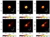 |
Fig. A.2 Radio maps of models RH1-100 observed at λ = 3.5 mm (ν = 86 GHz). Upper panels from left to right are models RH1, RH5, RH10 and lower panels from left to right are models RH20, RH40, RH100. |
All Tables
All Figures
|
Fig. 1 Dimensionless electron temperature, Θe = kTe/mec2, in the model with Rhigh = 1 (left panel) and Rhigh = 100 (middle panel). The right panel shows the proton-to-electron temperature ratio in the model with Rhigh = 100. The maps show the slices through the 3D GRMHD model (run b0-high in Table 5.1 in Shiokawa 2013) along the BH spin axis. |
| In the text | |
 |
Fig. 2 Same as in Fig. 1, but for the slices through the disk equatorial plane. |
| In the text | |
|
Fig. 3 Electromagnetic spectrum of GRMHD models computed at i = 20° and i = 90° based on models RH1-RH100 overplotted with the observations of M 87 collected in Abdo et al. (2009). Synchrotron emission appears in the SED as a hump around 230 GHz, and the higher order humps (second and third ones) are due to inverse-Compton emission. |
| In the text | |
|
Fig. 4 Intensity map of our fiducial model RH100 at λ = 7 mm (ν = 43 GHz) for a viewing angle of i = 20° (left panel) and i = 160° (right panel). The color scale is normalized to unity. See Table 1 for the total fluxes in units of Jansky for each model (Col. 7). The position angle of the jet axis/black hole spin is set to PA = 290° (Reid et al. 1982) E of N for both models. The size of each panel is 200 × 200 GMBH/c2 in the plane of the black hole. At a distance of D = 16.7 Mpc, this corresponds to an angular size of about 0.8 × 0.8 mas. |
| In the text | |
|
Fig. 5 Evolution of the intensity profile across (left panel) and along (right panel) the jet at λ = 7 mm (ν = 43 GHz). Color lines represent intensity at various times spaced by 20M ≡ 7 days. |
| In the text | |
|
Fig. 6 Contour maps of the model images (RH100) at λ = 7 mm (ν = 43 GHz) for viewing angles of i = 20° (left panel) and i = 160° (right panel) convolved with the telescope beam to simulate observations by Hada et al. (2011). The contour levels were chosen to match those from observations (contours decrease by a factor of 21 / 2 from the maximum intensity). The image size here is 480 × 480GMBH/c2 ≡ 1.8 × 1.8 mas, which is about twice the size used in Fig. 4 (images at λ = 7 mm). |
| In the text | |
|
Fig. 7 Same as Fig. 4 but for λ = 3.5 mm (ν = 86 GHz). Here the panel size is 100 × 100GMBH/c2 in the plane of the black hole, which corresponds to an angular size of about 480 × 480 μas. |
| In the text | |
|
Fig. 8 Intensity maps of model RH100 for i = 20° (upper left panel) and i = 160° (lower left panel) at λ = 1.3 mm (ν = 230 GHz). The total fluxes (at 1.3 mm) in these models are 1 Jansky. The position angle of the black hole spin is set to PA = 290° E of N for all models. The image size is 40 × 40 GMBH/c2 in the plane of the black hole, which at a distance of D = 16.7 Mpc, corresponds to an angular size of about 140 × 140 μas. Middle panels: the corresponding visibility amplitude on a u−v plane in units of Jy. Right panels: the visibility phase map in degrees. The arrows in the left and middle panels indicate the orientation of our coordinate system. |
| In the text | |
|
Fig. 9 Theoretical visibility amplitudes along E-W (left) and N-S (right) baselines, computed for model RH100 with i = 20°(solid lines) and 160°(dashed lines). |
| In the text | |
|
Fig. 10 Comparisons of the visibility amplitudes from our models and those from the EHT observations. The visibility amplitudes, computed at λ = 1.3 mm (ν = 230 GHz), along three baselines (SMT-CARMA, SMT-HAWAII, and CARMA-HAWAII) are shown for model RH100 with i = 20°(solid lines) and 160° (dashed lines). The distance between the VLBI stations is expressed in units of Mλ (1Mλ ≡ 1.3 km). The observed visibility amplitudes (points) and the u−v tracks are taken from Doeleman et al. (2012). |
| In the text | |
|
Fig. 11 43 GHz images of model RH100 observed at various inclination angles. |
| In the text | |
|
Fig. 12 Dimensionless electron temperature, Θe = kTe/mec2, in model RH100 overplotted with numerical grid. Maps show a cut through the 3D model along the BH spin axis. |
| In the text | |
|
Fig. A.1 Radio maps of models RH1-100 observed at λ = 1.3 mm (ν = 230 GHz). Upper panels from left to right are models RH1, RH5, RH10 and lower panels from left to right are models RH20, RH40, RH100. |
| In the text | |
|
Fig. A.2 Radio maps of models RH1-100 observed at λ = 3.5 mm (ν = 86 GHz). Upper panels from left to right are models RH1, RH5, RH10 and lower panels from left to right are models RH20, RH40, RH100. |
| In the text | |
Current usage metrics show cumulative count of Article Views (full-text article views including HTML views, PDF and ePub downloads, according to the available data) and Abstracts Views on Vision4Press platform.
Data correspond to usage on the plateform after 2015. The current usage metrics is available 48-96 hours after online publication and is updated daily on week days.
Initial download of the metrics may take a while.