| Issue |
A&A
Volume 585, January 2016
|
|
|---|---|---|
| Article Number | A118 | |
| Number of page(s) | 8 | |
| Section | Atomic, molecular, and nuclear data | |
| DOI | https://doi.org/10.1051/0004-6361/201527378 | |
| Published online | 06 January 2016 | |
Atomic data for astrophysics: Ni XII⋆
1
DAMTP, Centre for Mathematical Sciences, University of
Cambridge,
Wilberforce Road,
Cambridge
CB3 0WA,
UK
e-mail:
This email address is being protected from spambots. You need JavaScript enabled to view it.
2
Department of Physics, University of Strathclyde,
Glasgow, G4 0NG, UK
Received: 16 September 2015
Accepted: 5 November 2015
Abstract
We present new large-scale R-matrix (up to n = 4) scattering calculations for the electron collisional excitation of Cl-like Ni xii. We used the intermediate-coupling frame transformation method. We compare predicted and observed line intensities using laboratory and solar spectra, finding good agreement for all the main soft X-ray lines. With the exception of the three strongest transitions, large discrepancies with previous estimates are found, especially for the decays from the lowest 3s2 3p4 3d levels. This includes the forbidden UV lines. The atomic data for the n = 4 levels are the first to be calculated. We revise previous experimental energies, and suggest several new identifications. We point out the uncertainty in the wavelength of the 3s2 3p52P1/2–3s2 3p4 3d 2D3/2 transition, which is important for density diagnostics.
Key words: atomic data / techniques: spectroscopic / Sun: corona / line: identification
The full dataset is available at our APAP website (www.apapnetwork.org) and at the CDS via anonymous ftp to cdsarc.u-strasbg.fr (130.79.128.5) or via http://cdsarc.u-strasbg.fr/viz-bin/qcat?J/A+A/585/A118
© ESO, 2016
1. Introduction
Lines from Cl-like Ni xii are prominent in the soft X-rays and EUV (Gabriel et al. 1965). Several forbidden lines are also observed in the visible and UV part of the solar spectrum (Edlen & Smitt 1978). Nickel lines are also prominent in fusion plasma (see, e.g. Mattioli et al. 2004). Accurate atomic data are needed for this ion.
The most recent calculations for excitation by electron impact were carried out by Matthews et al. (1998). These authors included only the lowest 14 LS target states (31 fine-structure levels) of the 3s2 3p5, 3s 3p6, and 3s2 3p4 3d configurations in their close-coupling (CC) expansion. The CIV3 program was used to calculate the wave functions in LS coupling, and the R-matrix method (Berrington et al. 1995) was used to calculate the collision stengths in LS coupling. The j-resolved collision stengths were obtained using the JAJOM program (Saraph 1978).
The excitation rates calculated by Matthews et al. (1998) were supplemented with A-values and included in the CHIANTI database v.2 (Landi et al. 1999). They are still in the current v.8 of CHIANTI (Del Zanna et al. 2015). We note, however, that the excitation rates included in CHIANTI originated from a database that was held at Queen’s University of Belfast, and that some differences between the values in the database and those tabulated in Matthews et al. (1998) are present (E. Landi, priv. comm.).
Our recent large-scale atomic calculations for Cl-like Fe x (Del Zanna et al. 2012) have shown a significant improvement, compared to the previous smaller calculations (Del Zanna et al. 2004), in particular for the forbidden lines (see Del Zanna et al. 2014) and the decays from the 3s2 3p4 3d 4D , with typical changes larger than 50%. Del Zanna et al. (2012) included the full set of 32 configurations up to n = 4 in the configuration-interaction (CI) expansion and 218 LS terms in the CC expansion, i.e. much larger than the Matthews et al. (1998) calculation.
The aim of this paper is to present a large-scale calculation for Ni xii along the lines of the Fe x one, assess differences with the previous calculation, and benchmark the data against observations.
2. Atomic structure
The atomic structure calculations were carried out using the autostructure program (Badnell 2011) which constructs target wavefunctions using radial wavefunctions calculated in a scaled Thomas-Fermi-Dirac statistical model potential with a set of scaling parameters.
For the CI expansion we adopted the same set of 32 configurations up to n = 4 used for Fe x (Del Zanna et al. 2012), namely 3s2 3p5, 3s 3p6, 3s2 3p4 3d, 3s2 3p3 3d2, 3s 3p5 3d, 3p6 3d, 3p5 3d2 3s2 3p4 4l (l = s, p, d, f), 3s 3p5 4l (l = s, p, d, f), 3s2 3p3 3d 4l (l = s, p, d, f), 3p6 4l, 3p5 3d 4l (l = s, p, d, f). The scaling parameters λnl for the potentials in which the orbital functions are calculated are 1s: 1.40650, 2s: 1.12427, 2p: 1.06865, 3s: 1.17240, 3p: 1.14400, 3d: 1.17063, 4s: 1.17191, 4p: 1.14250, 4d: 1.15475, 4f: 1.28158.
Target level energies.
Ions such as Ni xii are particularly complex because of the strong mixing between levels having the same J-value and parity. The mixing between fine-structure levels substantially changes depending on the configurations included in the target representation, and, more importantly, on the relative position of the levels, which we improved with the term energy correction (TEC) method, introduced by Zeippen et al. (1977) and Nussbaumer & Storey (1978).
Unfortunately, only very few level energies are well known. We list the few experimental level energies Eexp in Table 1. From these, we obtained a set of “best guess” energies Ebest by linear interpolation. We then used the Ebest values to obtain the TEC values, then re-run autostructure to obtain the target energies ETEC, with the TEC applied. The ETEC and Eexp energies were used to calculate the radiative data.
We note that after having run the scattering calculations we have calculated the intensities of the strongest lines and then tentatively identified several levels, as we describe below. These tentative new energies are also listed in Table 1, with a “T” in the last column. We have not refined the TEC and re-run the calculations because of the uncertainty in the identifications of the lines and the corresponding level energies.
3. R-matrix scattering calculation
The R-matrix method used in the scattering calculation is described in Hummer et al. (1993) and Berrington et al. (1995). We performed the calculation in the inner region in LS coupling and included mass and Darwin relativistic energy corrections. The outer region calculation used the intermediate-coupling frame transformation method (ICFT) described by Griffin et al. (1998).
For the close-coupling expansion, we have retained the lowest 312 LS terms. This represents a significant improvement over the 14 LS target states included by Matthews et al. (1998), and an improvement over the 218 LS terms we included for Fe x (Del Zanna et al. 2012). We recall that Matthews et al. (1998) adopted the LS R-matrix + JAJOM programs.
Given that our CC expansion is much smaller than the CI expansion, the highest levels in the CC expansion do not have reliable collision strengths, mostly because of mixing with other levels not included in the CC expansion. We have calculated the collision strengths of the fine-structure levels associated with the 312 LS terms, but we only provide those associated with the lowest 589 levels, which include all the spectroscopically important levels (the No. 589 is the last 3s2 3p4 4f level).
Collision strengths for a selection of transitions.
The expansion of each scattered electron partial wave was done over a basis of 22 functions within the R-matrix boundary and the partial wave expansion extended to a maximum total orbital angular momentum quantum number of L = 16. This produced accurate collision strengths up to about 80 Ryd.
The outer region calculation includes exchange up to a total angular momentum quantum number J = 26/2. We have supplemented the exchange contributions with a non-exchange calculation extending from J = 28/2 to J = 74/2. Collision strengths were “topped-up” to infinite partial waves following Burgess (1974), Badnell & Griffin (2001).
The resonance region was calculated with 5400 points. A coarse energy mesh was chosen above all resonances.
To improve the collision strengths of the strongly mixed levels, we have included the TEC into the ICFT method as described in Del Zanna & Badnell (2014). This method can affect some decays from highly mixed levels. Table 2 lists a selection of collision strengths for the main transitions, for incident electron energies above thresholds, where resonance enhancements are not present.
Finally, the collision strengths were extended to high energies by interpolation using the appropriate high-energy limits in the Burgess & Tully (1992) scaled domain. The high-energy limits were calculated with autostructure (see Burgess et al. 1997; Chidichimo et al. 2003), including the TEC.
The temperature-dependent effective collisions strengths Υ(i − j) were calculated by assuming a Maxwellian electron distribution and linear integration with the final energy of the colliding electron. Figure 1 shows a few examples, compared to those calculated by Matthews et al. (1998) and those tabulated in the CHIANTI database. We only show a few collision strengths that are populating some of the most important levels, as described in the next Section. The plots in Fig. 1 show significant differences with those calculated by Matthews et al. (1998).
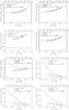 |
Fig. 1 Thermally-averaged collision strengths for a selection of transitions compared to those calculated by Matthews et al. (1998) and those tabulated in the CHIANTI database. |
A selection of the strongest Ni xii lines.
Some of the large differences in the thermally-averaged collision strengths are mostly present towards low temperatures, due to the resonance enhancements caused by our much larger CC expansion. Some examples are provided in the figure, the transitions to the 3s 3p62S1/2, 3s2 3p4 3d 4D5/2,7/2, and 3s2 3p4 3d 4F9/2 levels. In these three cases we note a discrepancy between the values published by Matthews et al. (1998) and the interpolated values in the CHIANTI database.
4. Comparison with observations
We have calculated the level populations using our collisions strengths and A-values. Proton excitation as available in the CHIANTI database v.8 (Del Zanna et al. 2015) has been included. The intensities of the strongest lines are shown in Table 3, for an electron density of 109 cm-3, typical of a solar active region, and the temperature of peak ion abundance in equilibrium. This table also shows in brackets the intensities as calculated with the CHIANTI database. There is relatively good agreement for the three strongest transitions; however, significant differences are found for all the other lines, in particular for the decays of the 3s2 3p4 3d 4D7/2,5/2. There are also significant enhancements in the forbidden lines.
We find good agreement between the predicted and observed intensities of the three main soft X-ray lines observed by Malinovsky & Heroux (1973) on the Sun, as shown in Fig. 2 (bottom). This figure shows the “emissivity ratio” curves 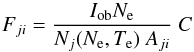 (1)for each line as a function of the electron density Ne. Iob is the observed intensity of the line (photon units), Nj(Ne,Te) is the population of the upper level j relative to the total number density of the ion, calculated at a fixed electron temperature Te = 1.8 MK, the temperature of peak ion abundance assuming ionization equilibrium. Aji is the spontaneous radiative transition probability, and C is a scaling constant chosen so the emissivity ratio is near unity. If agreement between experimental and theoretical intensities is present, all lines should be closely spaced. The crossing of the curves gives the electron density.
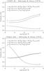 |
Fig. 2 Emissivity ratio curves relative to the soft X-ray solar Ni xii observed by Malinovsky & Heroux (1973). The observed intensities Iob are in ergs. The top plot is obtained with CHIANTI v.8, while the lower one with the present atomic data. |
The CHIANTI ion model has a small 20% discrepancy (see Fig. 2, top) in the ratio of the two strongest lines at 152.15 and 154.17 Å, decays from the 3s2 3p4 3d 2D5/2 (No. 29) and 3s2 3p4 3d 2P3/2 (No. 28) levels. The collision strengths of the allowed transitions to these levels are indeed similar to those calculated by Matthews et al. (1998; see top left plot of Fig. 1).
The 2–31 line is clearly blended in the Malinovsky & Heroux (1973) spectrum, and indeed the authors indicate that. The actual intensity of this line is likely to be lower, which would lower the emissivity curve of this line and lower the density. We note that the electron density obtained from the Fe xiv lines, which are formed over similar temperatures as Ni xii, is about 109 cm-3.
On the other hand, the CHIANTI ion model is inconsistent with the observations, as shown in Fig. 2 (top). The observed intensity of the 2–31 line would have to be twice the reported value. There is also a clear problem in the density sensitivity of the 2–31 line as calculated with the CHIANTI ion model. The upper level No. 31 (3s2 3p4 3d 2D3/2) is populated (at the density and temperature of the table) by direct excitation from the ground state 2P3/2 (49%) and the 2P1/2 (41%). As shown in Fig. 1, the stronger collision strengths from the 2P1/2 are in relative good agreement with the values calculated by Matthews et al. (1998); however, the collision strengths from the 2P3/2 are very much different. Our oscillator strength for the decay to the ground state does not vary much with the addition of the TEC, and is close to the value calculated by Fawcett (1987). Our collision strengths tend to the high-energy limits, so there seems to be a problem in the Matthews et al. (1998) calculations.
We now briefly comment on some significant differences in the predicted intensities of other lines, shown in Table 3. The 1−3 3s2 3p52P3/2–3s 3p62S1/2 transition is significantly enhanced. Only about 72% of the population of the upper level is due to direct excitation form the ground state, which is enhanced with the present calculation, as shown in Fig. 1. About 27% of its populations comes from cascading from higher levels which were not present in the previous atomic model. This is the reason for such a large difference, as we also found for Fe x (Del Zanna et al. 2012) and other coronal ions.
The 1–5 3s2 3p52P3/2–3s2 3p4 3d 4D7/2 is also very much enhanced in our model. It turns out that only 15% of its population comes from direct excitation form the ground state, which is enhanced with the present calculation, as shown in Fig. 1. About 84% comes from upper levels, for example 39% from level No. 9, 3s2 3p4 3d 4F9/2. In turn, this level No. 9 is populated by 15% from direct excitation form the ground state, which is enhanced with the present calculation, as shown in Fig. 1. The rest is due to cascading from higher levels, which are more populated because of increased collision strengths due to the larger number of resonances in our target.
Observed wavelengths of Ni xii lines.
4.1. A discussion on level energies and line identifications
We now briefly summarise the levels with known experimental energies. Table 4 lists the main wavelengths we have used to establish the experimental energies. The strongest Ni xii lines are produced by the 3s2 3p4 3d levels in the soft X-rays around 150 Å. The lines were identified by B.C. Fawcett (Gabriel et al. 1965, 1966; Fawcett & Hayes 1972), using laboratory spectra. These lines have been observed with high and moderate spectral resolution by sounding rocket flights in the 1960’s (Behring et al. 1972; Malinovsky & Heroux 1973). We adopt for the strongest lines the wavelength measurements of Sugar et al. (1992). We note a mistake in Sugar et al. (1992), the line observed at 159.970 Å is almost all due to Ni x, and not Ni xii. We also note that the wavelength of the 3s2 3p52P1/2–3s2 3p4 3d 2D3/2 (2–31) line is still somewhat uncertain, as we discuss below.
The forbidden line within the ground configuration was observed by Jefferies et al. (1971) during the 1965 eclipse. The decays from the 3s 3p62S1/2 level were identified by Fawcett & Hatter (1980).
Not all of the lower levels of the 3s2 3p4 3d configuration are known. Edlen & Smitt (1978) suggested the identification of several forbidden lines observed in the UV and visible. This established the energies of several levels (Nos. 9, 10, 18, 20, 21, 24, see Table 1) relative to the 3s2 3p4 3d 4D (level No. 5). The decay to the ground state from this 4D level is a relatively strong line with our new atomic data, so this line ought to be observable. We suggest that it is the line observed by Behring et al. (1976) at 220.247 Å. We base this suggestion on the differences between the observed and theoretical energy for this level that we obtained for Fe x, but also note that NIST suggests a similar energy. The theoretical splitting between the 4D level and the 4D
 (level No. 4) agrees within 200 Kaysers with the decay from the 4D level being the line observed by Behring et al. (1976) at 220.87 Å.
Finally, a few decays from 3s2 3p4 4s, 3s2 3p4 4d, 3s2 3p4 4f levels were identified by Fawcett et al. (1972) in the soft X-rays. As in the case of Fe x (Del Zanna et al. 2012), we predict that the decay from the 3s 3p5 4s 2P3/2 level to be stronger than the decays from the 3s2 3p4 4s. In the case of Fe x and the other coronal iron ions we were able to identify such soft X-ray transitions because they are relatively strong in solar spectra (Del Zanna 2012a), but in the case of nickel this is not simple.
4.1.1. The wavelength of the 3s2 3p52P1/2–3s2 3p4 3d 2D3/2 line
We note a puzzle regarding the wavelength of the 3s2 3p52P1/2–3s2 3p4 3d 2D3/2 (2–31) line. This line is weak at low densities, but becomes strong at high densities, as we have seen. Gabriel et al. (1965) identified this line with a laboratory line observed at 152.95 Å. The same identification is reported in Gabriel et al. (1966), Fawcett & Hayes (1972). Fawcett & Hayes (1972) actually report the observation of the decay to the ground state, at 147.60 Å.
Goldsmith & Fraenkel (1970) used a vacuum spark and remeasured the nickel lines, providing a different identification for the 2–31 line, observed at 153.174 Å. The decay to the ground state was listed with zero intensity at 147.847 Å (we note that the other lines had similar wavelengths to those measured by Fawcett).
However, the branching ratio of the two decays is 0.024, i.e. the decay to the ground state is only 2.4% the intensity of the 2–31 line. So it is questionable that the decay to the ground state was actually observed by Fawcett or Goldsmith & Fraenkel (1970). We return to this issue below.
Several laboratory spectra followed (see e.g. Wouters et al. 1988; Mattioli et al. 2004), but they did not have a sufficiently high spectral resolution to settle this issue. Mattioli et al. (2004) noted that the wavelength of the 2–31 line is consistent with the Fawcett measurement. Surprisingly, Sugar et al. (1992) does not list this transition. Keenan et al. (2000) reported observations with the Joint European Torus (JET) tokamak, and a wavelength of 152.90 Å for this line. However, we note that the profile of this line in the JET spectra looks asymmetric and the spectrometer used had a medium resolution of 0.2 Å.
To help resolve the issue we have considered the excellent vacuum spark spectra obtained by Ryabtsev (1979). The spectrograph used for the measurements had a radius of 3 m, so these spectra are the best in terms of spectral resolution. Lines from titanium were used as reference to establish the wavelength calibration. The Ryabtsev (1979) wavelengths of the strongest Ni xii lines are in agreement with those of Sugar et al. (1992) within a few mÅ.
Ryabtsev (1979) report observations of nickel lines produced by a low-induction vacuum spark, with two settings. With the “cold” setting only low charge states of nickel were present. With the “hot” setting, higher ionization stages such as Ni xii were present. The lines that are known to pertain to lower charge-state ions such as Ni x have intensities that do not change much from the “cold” to the “hot” spectrum. Several of the Ni xii lines are clearly blended with lower charge-state ions, since they have considerable intensities in the “cold” spectrum. If we assume that no blending from higher ionization stages is present, and remove the lower charge-state contribution by subtracting the intensities of the “cold” spectrum from the “hot” spectrum, we obtain the emissivity ratio curves shown in Fig. 3. The agreement between predicted and observed intensities is truly remarkable, within only 20% at high densities, as we would expect in the vacuum spark spectra (the level populations reach Boltzmann equilibrium around 1011 cm-3).
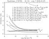 |
Fig. 3 Emissivity ratio curves relative to the soft X-ray Ni xii observed by Ryabtsev (1979). |
Ryabtsev (1979) observed a line at 147.820 Å, which is listed as the same line observed by Goldsmith & Fraenkel (1970) at 147.847 Å. As the Fig. 3 shows, this line cannot be the decay of the 3s2 3p4 3d 2D3/2 to the ground state, having an intensity about a factor of six too high, as we anticipated. This means that the previous wavelenghts of the decay to the 3s2 3p52P1/2 level (the 2–31 transition) based on the decay to the ground state should be treated with caution.
With regard to the 2–31 transition itself, Ryabtsev (1979) lists four nickel lines around 153 Å, at 152.697, 152.833, 152.929, and 153.177 Å. The line at 152.833 Å is listed as a possible Ni xi line, because of its intensity in the cold and hot spectra. Its intensity is a factor of two too low compared to our prediction, so we discard it as a possible candidate. The line at 153.177 Å is clearly the same line observed by Goldsmith & Fraenkel (1970) at 153.174 Å. However, it is unlikely that this line is the 2–31 transition, because its observed intensity is also too low.
We are then left with two possibilities, the lines at 152.697 and 152.929 Å. These lines have similar intensities, and would be blended in most medium-resolution spectra, including the solar one of Malinovsky & Heroux (1973), and the JET tokamak (Keenan et al. 2000; Mattioli et al. 2004). We have re-measured the wavelength of the line observed in the Malinovsky & Heroux (1973) spectrum, obtaining a value of 152.80 ± 0.10 Å, i.e. in between the two wavelengths of the candidate lines observed by Ryabtsev (1979).
However, the 152.697 and 152.929 Å lines would be well separated in the high-resolution solar spectrum of Behring et al. (1972). These authors only list one unidentified line at 152.703 Å, a wavelength very close to 152.697 Å. We therefore suggest this new identification. We note that most of the lines listed by Ryabtsev (1979) would not be observable in the low-density solar corona, but the 2–31 transition should be, although the approximate intensity given by Behring et al. (1972) to the 152.703 Å line is larger than what it should be.
Our suggestion is also supported by its predicted wavelength based on the theoretical splitting between the 3s2 3p4 3d 2D5/2,3/2 levels. The observed energy of the 2D5/2 level is 710 cm-1 higher than the theoretical energy obtained with the TEC (cf. Table 1). If the 153.177 Å line was the 2–31 transition, the energy of the 2D3/2 level would be 1916 cm-1 lower than predicted. If the 152.929 Å line was the 2–31 transition, the energy of the 2D3/2 level would be 857 cm-1 lower than predicted. In the case of the 152.697 Å line, the energy of the 2D3/2 level would be instead 136 cm-1 higher than predicted, in closer agreement with the energy of the 2D5/2 level. We note, however, that these levels are strongly mixed as shown in Table 1, so there is some uncertainty in the above arguments.
4.1.2. Other tentative identifications
Finally, Table 3 shows that there are several lines that fall around 190 Å and should be observable, although very weak. Several unidentified nickel lines in the EUV were observed by Beiersdorfer et al. (2014), Träbert et al. (2014) with an electron beam ion trap (EBIT), however none of them appear to be due to Ni xii.
Several coronal unidentified lines have also been observed by Del Zanna (2012b) with the Hinode EUV imaging spectrometer (EIS, see Culhane et al. 2007) in an active region. We have assumed the CHIANTI ion fractions and performed an emission measure analysis to estimate the count rates in the Ni xii that are predicted at the Hinode EIS wavelengths for the active region discussed in Del Zanna (2012b). The intensities of the strongest Ni xii lines are close to the weakest lines observed by EIS, so it is not easy to establish any identifications.
We suggest a few tentative identifications, on the following grounds: 1) the energies are close to those we expect based on the TEC of other levels; 2) the lifetimes of the levels were observed by Trabert et al. (1993) with beam-foil spectroscopy; 3) the predicted intensities are close to the observed ones. The decay from level No. 19 (2D5/2) was observed around 193.3 Å by Trabert et al. (1993). The Hinode EIS spectrum has a weak line at 193.218 Å. The decay from level No. 22 (2F5/2) was observed around 189.3 Å by Trabert et al. (1993). The Hinode EIS spectrum has a weak line at 189.26 Å. The decay from level No. 14 (4F5/2) was observed around 202 Å by Trabert et al. (1993). The decay from level No. 16 (4P3/2) was observed around 198.2 Å by Trabert et al. (1993). The Hinode EIS spectrum has a weak line at 198.289 Å.
5. Conclusions
As in the case of the Cl-like Fe x (Del Zanna et al. 2012), we have found that a large-scale R-matrix calculation for Ni xii produces significant enhancements in the intensities of all the transitions that originate from the lower levels. These results are similar to those we obtained for Fe x (Del Zanna et al. 2012), as briefly outlined in the introduction. They are partly due to resonance enhancement of the collision strengths, and partly due to increased population via cascading from higher levels. We have found similar enhancements for other coronal iron ions.
However, in some cases large differences are not simply due to the resonance enhancement but to the different CI expansion. Overall, the present data provide line intensities that are largely different than previous estimates based on the Matthews et al. (1998) calculations.
For Fe x, we were able to use laboratory plates and solar spectra to identify many of the levels of the 3s2 3p4 3d configuration (Del Zanna et al. 2004). However, for Ni xii this has not been possible. We have suggested several new identifications that have experimental energies close to our estimated ones with the use of the TEC, but they need to be confirmed with more accurate experimental data. Therefore, the adjustments to our calculations via the TEC could be improved in the future if further levels are firmly identified.
We have provided a set of complete atomic data which can be used to aid the identification process using laboratory data. In particular, further high-resolution observations would be useful to clarify the wavelength of the 3s2 3p52P1/2–3s2 3p4 3d 2D3/2 transition.
Acknowledgments
The present work was funded by STFC (UK) through the University of Cambridge DAMTP astrophysics grant and the University of Strathclyde UK APAP network grant ST/J000892/1.
References
- Badnell, N. R. 2011, Comp. Phys. Comm., 182, 1528 [Google Scholar]
- Badnell, N. R., & Griffin, D. C. 2001, J. Phys. B Atom. Mol. Phys., 34, 681 [Google Scholar]
- Behring, W. E., Cohen, L., & Feldman, U. 1972, ApJ, 175, 493 [NASA ADS] [CrossRef] [Google Scholar]
- Behring, W. E., Cohen, L., Doschek, G. A., & Feldman, U. 1976, ApJ, 203, 521 [NASA ADS] [CrossRef] [Google Scholar]
- Beiersdorfer, P., Träbert, E., Lepson, J. K., Brickhouse, N. S., & Golub, L. 2014, ApJ, 788, 25 [NASA ADS] [CrossRef] [Google Scholar]
- Berrington, K. A., Eissner, W. B., & Norrington, P. H. 1995, Comput. Phys. Comm., 92, 290 [Google Scholar]
- Burgess, A. 1974, J. Phys. B Atom. Mol. Phys., 7, L364 [Google Scholar]
- Burgess, A., & Tully, J. A. 1992, A&A, 254, 436 [NASA ADS] [Google Scholar]
- Burgess, A., Chidichimo, M. C., & Tully, J. A. 1997, J. Phys. B Atom. Mol. Phys., 30, 33 [NASA ADS] [CrossRef] [Google Scholar]
- Chidichimo, M. C., Badnell, N. R., & Tully, J. A. 2003, A&A, 401, 1177 [NASA ADS] [CrossRef] [EDP Sciences] [Google Scholar]
- Culhane, J. L., Harra, L. K., James, A. M., et al. 2007, Sol. Phys., 243, 19 [Google Scholar]
- Del Zanna, G. 2012a, A&A, 546, A97 [NASA ADS] [CrossRef] [EDP Sciences] [Google Scholar]
- Del Zanna, G. 2012b, A&A, 537, A38 [NASA ADS] [CrossRef] [EDP Sciences] [Google Scholar]
- Del Zanna, G., & Badnell, N. R. 2014, A&A, 570, A56 [NASA ADS] [CrossRef] [EDP Sciences] [Google Scholar]
- Del Zanna, G., Berrington, K. A., & Mason, H. E. 2004, A&A, 422, 731 [NASA ADS] [CrossRef] [EDP Sciences] [Google Scholar]
- Del Zanna, G., Storey, P. J., Badnell, N. R., & Mason, H. E. 2012, A&A, 541, A90 [NASA ADS] [CrossRef] [EDP Sciences] [Google Scholar]
- Del Zanna, G., Storey, P. J., Badnell, N. R., & Mason, H. E. 2014, A&A, 565, A77 [NASA ADS] [CrossRef] [EDP Sciences] [Google Scholar]
- Del Zanna, G., Dere, K. P., Young, P. R., Landi, E., & Mason, H. E. 2015, A&A, 582, A56 [NASA ADS] [CrossRef] [EDP Sciences] [Google Scholar]
- Edlen, B., & Smitt, R. 1978, Sol. Phys., 57, 329 [NASA ADS] [CrossRef] [Google Scholar]
- Fawcett, B. C. 1987, Atom. Data and Nuclear Data Tables, 36, 151 [Google Scholar]
- Fawcett, B. C., & Hatter, A. T. 1980, A&A, 84, 78 [NASA ADS] [Google Scholar]
- Fawcett, B. C., & Hayes, R. W. 1972, J. Phys. B Atom. Mol. Phys., 5, 366 [Google Scholar]
- Fawcett, B. C., Cowan, R. D., & Hayes, R. W. 1972, J. Phys. B Atom. Mol. Phys., 5, 2143 [NASA ADS] [CrossRef] [Google Scholar]
- Gabriel, A. H., Fawcett, B. C., & Jordan, C. 1965, Nature, 206, 390 [NASA ADS] [CrossRef] [Google Scholar]
- Gabriel, A. H., Fawcett, B. C., & Jordan, C. 1966, Proc. Phys. Soc., 87, 825 [NASA ADS] [CrossRef] [Google Scholar]
- Goldsmith, S., & Fraenkel, B. S. 1970, ApJ, 161, 317 [NASA ADS] [CrossRef] [Google Scholar]
- Griffin, D. C., Badnell, N. R., & Pindzola, M. S. 1998, J. Phys. B Atom. Mol. Phys., 31, 3713 [Google Scholar]
- Hummer, D. G., Berrington, K. A., Eissner, W., et al. 1993, A&A, 279, 298 [NASA ADS] [Google Scholar]
- Jefferies, J. T., Orrall, F. Q., & Zirker, J. B. 1971, Sol. Phys., 16, 103 [NASA ADS] [CrossRef] [Google Scholar]
- Keenan, F. P., Botha, G. J. J., Matthews, A., Lawson, K. D., & Coffey, I. H. 2000, MNRAS, 318, 37 [NASA ADS] [CrossRef] [Google Scholar]
- Landi, E., Landini, M., Dere, K. P., Young, P. R., & Mason, H. E. 1999, A&AS, 135, 339 [NASA ADS] [CrossRef] [EDP Sciences] [Google Scholar]
- Malinovsky, L., & Heroux, M. 1973, ApJ, 181, 1009 [NASA ADS] [CrossRef] [Google Scholar]
- Matthews, A., Ramsbottom, C. A., Bell, K. L., & Keenan, F. P. 1998, Atom. Data and Nuclear Data Tables, 70, 41 [NASA ADS] [CrossRef] [Google Scholar]
- Mattioli, M., Fournier, K. B., Coffey, I., et al. 2004, J. Phys. B Atom. Mol. Phys., 37, 13 [NASA ADS] [CrossRef] [Google Scholar]
- Nussbaumer, H., & Storey, P. J. 1978, A&A, 64, 139 [NASA ADS] [Google Scholar]
- Ryabtsev, A. N. 1979, Sov. Astron., 23, 732 [NASA ADS] [Google Scholar]
- Sandlin, G. D., & Tousey, R. 1979, ApJ, 227, L107 [NASA ADS] [CrossRef] [Google Scholar]
- Sandlin, G. D., Brueckner, G. E., & Tousey, R. 1977, ApJ, 214, 898 [NASA ADS] [CrossRef] [Google Scholar]
- Saraph, H. E. 1978, Comput. Phys. Comm., 15, 247 [NASA ADS] [CrossRef] [Google Scholar]
- Sugar, J., Kaufman, V., & Rowan, W. L. 1992, J. Opt. Soc. Am. B Opt. Phys., 9, 344 [NASA ADS] [CrossRef] [Google Scholar]
- Trabert, E., Brandt, M., Doerfert, J., et al. 1993, Phys. Scr, 48, 580 [NASA ADS] [CrossRef] [Google Scholar]
- Träbert, E., Beiersdorfer, P., Brickhouse, N. S., & Golub, L. 2014, ApJS, 215, 6 [NASA ADS] [CrossRef] [Google Scholar]
- Wouters, A. W., Schwob, J. L., Suckewer, S., et al. 1988, J. Opt. Soc. Am. B Opt. Phys., 5, 1520 [NASA ADS] [CrossRef] [Google Scholar]
- Zeippen, C. J., Seaton, M. J., & Morton, D. C. 1977, MNRAS, 181, 527 [NASA ADS] [CrossRef] [Google Scholar]
All Tables
All Figures
|
Fig. 1 Thermally-averaged collision strengths for a selection of transitions compared to those calculated by Matthews et al. (1998) and those tabulated in the CHIANTI database. |
| In the text | |
|
Fig. 2 Emissivity ratio curves relative to the soft X-ray solar Ni xii observed by Malinovsky & Heroux (1973). The observed intensities Iob are in ergs. The top plot is obtained with CHIANTI v.8, while the lower one with the present atomic data. |
| In the text | |
|
Fig. 3 Emissivity ratio curves relative to the soft X-ray Ni xii observed by Ryabtsev (1979). |
| In the text | |
Current usage metrics show cumulative count of Article Views (full-text article views including HTML views, PDF and ePub downloads, according to the available data) and Abstracts Views on Vision4Press platform.
Data correspond to usage on the plateform after 2015. The current usage metrics is available 48-96 hours after online publication and is updated daily on week days.
Initial download of the metrics may take a while.