| Issue |
A&A
Volume 584, December 2015
|
|
|---|---|---|
| Article Number | A40 | |
| Number of page(s) | 12 | |
| Section | Stellar structure and evolution | |
| DOI | https://doi.org/10.1051/0004-6361/201526102 | |
| Published online | 18 November 2015 | |
2MASS J22560844+5954299: the newly discovered cataclysmic star with the deepest eclipse⋆,⋆⋆
1
Department of PhysicsFaculty of Natural Sciences, Shumen University, 115
Universitetska Str.,
9712
Shumen,
Bulgaria
e-mail:
d.kyurkchieva@shu-bg.net
2
Moscow MV Lomonosov State University, Sternberg Astronomical
Institute, 13 Universitetskii pr., 119991
Moscow,
Russia
3
Institute of Astronomy and National Astronomical Observatory,
Bulgarian Academy of Sciences, 72
Tsarigradsko Shose Blvd., 1784
Sofia,
Bulgaria
4
Bundesdeutsche Arbeitsgemeinschaft für Veränderliche Sterne e.V.
(BAV) Munsterdamm 90, 12169
Berlin,
Germany
Received: 16 March 2015
Accepted: 12 August 2015
Context. The SW Sex stars are assumed to represent a distinguished stage in cataclysmic variable (CV) evolution, making it especially important to study them.
Aims. We discovered a new cataclysmic star and carried out prolonged and precise photometric observations, as well as medium-resolution spectral observations. Modelling these data allowed us to determine the physical parameters and to establish its peculiarities.
Methods. To obtain a light curve solution we used model whose emission sources are a white dwarf surrounded by an accretion disk with a hot spot, a gaseous stream near the disk’s lateral side, and a secondary star filling its Roche lobe. The obtained physical parameters are compared with those of other SW Sex-subtype stars.
Results. The newly discovered cataclysmic variable 2MASS J22560844+5954299 shows the deepest eclipse amongst the known nova-like stars. It was reproduced by totally covering a very luminous accretion disk by a red secondary component. The temperature distribution of the disk is flatter than that of steady-state disk. The target is unusual with the combination of a low mass ratio q ~ 1.0 (considerably below the limit q = 1.2 of stable mass transfer of CVs) and an M-star secondary. The intensity of the observed three emission lines, Hα, He 5875, and He 6678, sharply increases around phase 0.0, accompanied by a Doppler jump to the shorter wavelength. The absence of eclipses of the emission lines and their single-peaked profiles means that they originate mainly in a vertically extended hot-spot halo. The emission Hα line reveals S-wave wavelength shifts with semi-amplitude of around 210 km s-1 and phase lag of 0.03.
Conclusions. The non-steady-state emission of the luminous accretion disk of 2MASS J22560844+5954299 was attributed to the low viscosity of the disk matter caused by its unusually high temperature. The star shows all spectral properties of an SW Sex variable apart from the 0.5 central absorption.
Key words: binaries: eclipsing / stars: individual: 2MASS J22560844+5954299 / novae, cataclysmic variables / white dwarfs / accretion, accretion disks
Spectra (FITS files) are only available at the CDS via anonymous ftp to cdsarc.u-strasbg.fr (130.79.128.5) or via http://cdsarc.u-strasbg.fr/viz-bin/qcat?J/A+A/584/A40
© ESO, 2015
1. Introduction
The cataclysmic variables (CVs) consist of a white dwarf and a late main-sequence (MS) star filling its Roche lobe. The white dwarfs of the most CVs (excluding polars) are surrounded by accretion disks. The disk and/or the hot spot are dominant sources of their optical emission. These systems are natural laboratories for accretion-disk physics because the timescale of their accretion is relatively short compared to other accreting objects. Cataclysmic variables are the closest systems whose mass outflows are associated with accretion via a disk onto compact objects (Noebauer et al. 2010).
The nova-like (NLs) stars are nonmagnetic cataclysmic variables that do not show large variations like dwarf nova outbursts. Their main photometric characteristics are small humps and reduced flickering, while their optical spectra are dominated by wide Balmer emission lines and HeI/HeII emission lines (for a comprehensive description of NLs and their emission sources, see the books of Warner 1995; and Hellier 2001). Most nova-like variables have orbital periods just above the period gap where magnetic braking from the secondary star (Howell et al. 2001) is thought to be the dominant mechanism for angular momentum loss and to have a much stronger effect than gravitational radiation (which is thought to be dominant below the gap). This naturally explains the high mass-transfer rates above the gap (although one has to keep in mind that there are also dwarf novae above the gap). It is assumed that the NLs are in a state of “permanent eruption” because of their high accretion rate, producing largely ionized accretion disks in which the viscous-thermal instability (driving dwarf nova limit cycles) is suppressed (Osaki 2005). Because they stay in the high mass-transfer state for long periods of time, they may be the closest examples of steady-state accretion disks among the CVs.
A quarter century ago, a sub-class of NLs, called “SW Sex stars”, was identified (Szkody & Piche 1990; Thorstensen et al. 1991a; Dhillon et al. 2013) with contradictory properties: deep continuum eclipses (with unusual V-shaped profiles) that imply a high-inclination accretion disc and emission lines with single-peaked profiles and shallow eclipses, instead of the deeply eclipsing, double-peaked profiles one would expect (Horne & Marsh 1986). Moreover, their emission lines do not reflect the orbital motion of the white dwarf (there is a substantial orbital phase lag of ~0.2 cycle) and exhibit transient absorption features around phase 0.5, all indicative of a complex, possibly non-disk origin. Different mechanisms were proposed to explain the behaviour of the SW Sex stars (Hellier & Robinson 1994; Williams 1989; Casares et al. 1996; Horne 1999; Knigge et al. 2000). But their unusually high luminosities and accretion geometry still do not have a satisfactory explanation (Townsley & Bildsten 2003; Townsley & Gansicke 2009; Ballouz & Sion 2009, etc.).
The recent observations revealed that the SW Sex stars represent dominant fraction of all CVs in the orbital period range 3−4 h (Rodriguez-Gil et al. 2007). The prototypical NL UX UMa occasionally also exhibits SW Sex-like behavior (Neustroev et al. 2011). Dhillon et al. (2013) propose that all NLs (excepting VY Sct subtype) be classified as SW Sex stars. On the other hand, models imply that CVs evolve from longer to shorter orbital periods, driven by angular momentum loss, which means that CVs that formed with periods more than 4 h will eventually pass through the 3−4 h regime. Since most CVs in that range appear to be SW Sex stars, it is reasonable to assume that systems that evolve into that range will turn into SW Sex stars, meaning that the SW Sex phenomenon could be considered as an evolutionary stage of the CV population. The exclusive evolution role makes the SW Sex stars important astrophysical objects. Although the eclipses are no longer required to belong to the SW Sex subtype, the eclipsing SW Sex systems are of particular interest, since time-resolved observations of the eclipse provide spatial information about the disk and physical parameters of their configurations (Dhillon et al. 2013).
In this paper we report the results of our study of a newly discovered SW Sex star with deep eclipse. They are based on seven-year photometry and medium-resolution spectroscopy covering the whole orbital cycle.
2. Discovery and first observations
The photometric variability of the star GSC1 03997 00231 was discovered in 2008 during observations of NGC 7429 by an eight-inch telescope at a private observatory near Nürnberg (Groebel 2009). They revealed light minima with depth 0.4−0.5 mag and duration around 1 h repeating every 5.5 h. The initial supposition was that it is an eclipsing system consisting of two almost equal dwarf stars with orbital period of near 11 h.
GSC1 03997 00231 seemed elongated on the first low-resolution CCD images (as well as on the POSS and SDSS images). The GSC 2.3 catalogue gave the reason: there were two stars at this position at 6 arcsec separation from each other: N1CB000021 (the brighter one, 2MASS J22560768+5954286, RA = 22 56 07.68, Dec = +59 54 28.7) and N1CB002289 (the fainter one, RA = 22 56 08.44, Dec = +59 54 29.98). The next Nürnberg observations identified the fainter star as the variable one. Its designation is 2MASS J22560844+5954299, so from now on we use the shorter name J2256.
J2256 was observed regularly during 2008−2009 by the eight-inch Meade telescope and CCD camera ST6 without filter (in a semi-automated mode) and by the ten-inch telescope with ST8 camera during 2010−2012. The exposures were 60 s. The reduction of images (dark and flat field corrections) were performed by the software Muniwin (Motl 2012). An aperture of five-pixel radius corresponding to a 7.5 arcsec sky field was used for photometry. The comparison stars were selected to be similar to the variable star in magnitude and spectral type (estimated by the 2MASS (J − K) index) and to be constant within the photometric error of 0.02 mag.
The times of the individual minima were determined by the method of Kwee & van Woerden (1956). The linear fit of the obtained 73 times of eclipse minima from 2008−2012 led to the ephemeris  (1)The intensive Nürnberg observations exhibited changes both in the minimum depths and out-of-eclipse shape and in the asymmetry of the eclipses (Fig. 1). These characteristics indicated a nova-like eclipsing cataclysmic variable rather than a detached eclipsing system. The V-shaped light minimum, as well as the presence of “shoulder” on the increasing branch of some light curves, supported this supposition (Fig. 1). The star (IPHAS J225608.45+595430.0) in the IPHAS catalogue (of H-alpha emission lines source) was another indication of its classification as a cataclysmic variable (Witham et al. 2008).
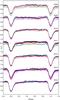 |
Fig. 1 Representative (annual) samples of the numerous Nürnberg unfiltered light curves of J2256 during 2008−2014 (the symbol sizes correspond to the photometric error of around 0.02 mag). |
To study this newly discovered cataclysmic variable we undertook follow-up photometric and spectroscopic observations at the Rozhen observatory.
Journal of the Rozhen observations.
3. Rozhen observations
The photometric observations of J2256 at the Rozhen National Astronomical Observatory were carried out with (i) the 60-cm Cassegrain telescope using the FLI PL09000 CCD camera (3056 × 3056 pixels, 12 μm/pixel, field of 27.0 × 27.0 arcmin with focal reducer); and (ii) the 2-m RCC telescope with the CCD camera VersArray 1300B (1340 × 1300 pixels, 20 μm/pixel, diameter of field of 15 arcmin).
Table 1 presents a journal of the Rozhen observations obtained under good atmospheric conditions (seeing 1−2 arcsec) and covering at least a cycle. Their average accuracy (Table 1) became three to four times bigger at the bottom of the eclipses.
The standard IDL procedures (adapted from DAOPHOT) were used for reducing the photometric data. All frames are dark-frame-subtracted and flat-field-corrected. They were analyzed using an aperture of 3 arcsec. The comparison stars (Table 2) were selected to fulfil the requirement of being constant within 0.01 mag during all observational runs and in all filters.
The spectral observations of J2256 were carried by the 2 m RCC telescope equipped with the focal reducer FoReRo 2 and grism with 720 lines/mm. The resolution of the spectra is 2 pix or 2.7 Å and they cover the range 5600−7000 Å. Most of the spectra have a S/N of 16−22 excluding those at the eclipse where the S/N value is around 7. The spectra were reduced using IRAF packages for bias subtraction, flat-fielding, cosmic ray removal, and one-dimensional spectrum extraction. For wavelength calibration, we used 30 appropriate night-sky emission lines from the spectral atlas of Osterbrock et al. (1996). They were fitted by third-order polynomials and the resulting dispersion curve was with rms ~ 0.2 Å. The spectra were normalized by dividing by the continuum value around 6500 Å.
4. Analysis of the photometric data
4.1. Initial analysis
To determine the eclipse timings of the Rozhen photometric data and their errors, we fitted the eclipses by the function Pearson IV of the software Table curve 2D (Systat Software, Inc.). The linear fit of all Nürnberg eclipse timings, including the later ones from 2013−2014 (Fig. 1), as well as those from the precise Rozhen photometry, led to improving the target period and led to a new ephemeris:  (2)whose initial epoch corresponds to the first observed minimum at Rozhen.
Coordinates and magnitudes of the comparison stars for the data of the 60 cm telescope.
Parameters of the Rozhen light curves.
We phased the Rozhen photometric observations with the ephemeris (2). Table 3 presents information on the sample consisting of two light curves in each filter (indexed by “1” and “2”) obtained by the 60 cm telescope and separated by at least approximately two months. The columns of Table 3 are as follows: set designation; NN(1) − number of the orbital cycle according to the ephemeris (1); NN(2) − number of the orbital cycle according to the ephemeris (2); date; t1, t2− times of the beginning and end of the observations; ϕ1, ϕ2− phases of the beginning and end of the observations according to (2); Tmin− time of the observed minimum; mmax and mmin− visual magnitudes corresponding to the maximum and minimum brightness during the corresponding set of observations.
The qualitative analysis of the Rozhen BVRI light curves (Fig. 2) led us to several conclusions. (i) There are changes of the light curves of the two filter sets by ~0.06−0.14 mag (bigger in V and I bands). (ii) The eclipse depths of the Rozhen data are considerably bigger (by a factor of 4−8) than those of the Nürnberg ones (Fig. 1). This effect is due to the low spatial resolution of the Nürnberg observations, leading to considerable light contribution of the neighbouring star and thus to reducing of the true amplitude of variability. (iii) There is no pre-eclipse hump, except a light curve B1 with a weak hump (Fig. 2). (iv) The light level after the eclipse is lower than the level before it. (v) There is a prolonged plateau outside the eclipse in filters B and V.
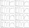 |
Fig. 2 a) Rozhen photometric data of J2256 (points with the corresponding error bars), the synthetic light curves (continuous lines), and the corresponding residuals; b) details around the eclipse minima (the error bars are smaller than the symbol size); c) details of the out-of-eclipse parts of light curves. |
The most distinguishable feature of J2256 is its deep eclipse: ~4 mag in V. The eclipse depths of the majority of the eclipsing nova-like variables are ≤1 mag. The deepest eclipses belong to the SW Sex stars. Only nine SW Sex stars in the list of Rodriguez-Gil et al. (2007) have eclipse depths more than 2.0 mag (Khruzina et al. 2013). Two SW Sex stars, DW UMa (Stanishev et al. 2004) and V1315 Aql (Papadaki et al. 2009), normally have eclipse depths less than 2.0 mag, but on rare occasions and only within two to three days do they show deeper eclipses of 3.2−3.4 mag. Dimitrov & Kjurkchieva (2012) report the SW Sex star 2MASS J01074282+4845188 with an eclipse depth of V ~ 2.9 mag, but the newly discovered cataclysmic star J2256 turned out to have an even deeper eclipse. In fact, it shows the deepest eclipse among the known eclipsing nova-like variables.
4.2. Light curve solution
The shapes of the J2256 light curves are typical of nova-like CVs. Particularly, 2MASS J01074282 + 4845188, observed by us with the same equipment, has a similar light curve (Khruzina et al. 2013). That is why we used the model applied successfully for other cataclysmic variables to determine the system parameters of J2256. A detailed description is given in Khruzina (1998, 2011). The configuration consists of a white dwarf and late-type secondary filling of its Roche lobe. The shape of the secondary is determined by the Roche potential. The effects of gravitational darkening and non-linear limb darkening are taken into account when calculating the emission of its surface elements. The emission of the white dwarf with radius Rwd is assumed for the black-body type that corresponds to effective temperature Twd. It is surrounded by an opaque, slightly elliptical accretion disk, coplanar to the orbital plane of the system. The outer (lateral) surface of the unperturbed disk presents part of ellipsoid with semi-axes a,b,c, while its inner surfaces are parts of two paraboloids with parameter A. The thickness of the disk outer edge βd is specified by the parameters a and A. Another geometrical parameter ξ(q), which was used in the solution, represents the distance between the centre of the white dwarf and L1. The collision of the gas stream from the secondary with the rotating disk results in formation of hot spot described by a half ellipse. All linear sizes of the model are in units of the binary separation a0. Furthermore, we use the unit ξ to express the disk radius in order to compare it to similar structures in other CVs (see Sect. 4.3). Moreover, ξ turns out to be a useful parameter at the first stage of the light curve solution when the mass ratio is unknown, and ξ serves to set the possible ranges for varying Rwd and Rd. (If they were in a0 there is a considerable probability the component sizes to exceed the Roche lobe that will cause stop of the calculations.)
Depths and widths of the eclipse.
The fluxes from the differential emitting areas are in conditional units because the Planck function gives the flux from 1 cm2 per unit wavelength range (in our case, centimetre), while the linear measure of the code for the light curve synthesis is the distance a0, whose value is not known in advance.
The temperature profile of the disk is determined by the parameter αg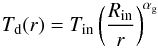 (3)(αg = 0.75 corresponds to the equilibrium state of the disk).
While the traditional models of CVs assume that the gas stream is transparent to the emission of the shock wave, and the heated region, called a “hot spot”, is the area of the interaction of the stream with the disk, the gas stream is opaque in our model. As a result, the heated region, analogue of the “classical” hot spot, consists of two components (Fig. 3): part of the hot line near the disk and disk region at the leeward side of the hot line.
The optically opaque part of the gas stream, the hot line, is approximated by part of the elongated ellipsoid with axes av,bv,cv. Its major axis bv coincides with the axis of the gas stream from the inner Lagrange point L1. The temperature of the hot-line surface changes according to a cosine law (for details, see Khruzina 2011):  (4)where ΔTww,max and ΔTlw,max are the maximum corrections to the disk temperature Td(r) corresponding to the windward and leeward sides near the disk, δr is the distance of the current hot-line point from the disk edge, and n is for ww or lw. The local temperature at the disk area inside the hot spot varies by a cosine law with the maximum value at the point U of the intersection between the hot-line axis and the disk.
The adjustable parameters of the light curve solution were: (a) parameters of the stellar components: mass ratio q = Mwd/Mred; orbital inclination i; effective temperatures of the white dwarf Twd and red star Tred; radius of the white dwarf Rwd; (b) parameters of the accretion disk: temperature Tin of the inner region (boundary layer); eccentricity e (e ≤ 0.1); large semiaxis a; parameter αg defining the temperature distribution along its radius; azimuth of the disk periastron αe; parameter of the paraboloid surface A (the thickness of the outer disk edge βd = f(A, a) is calculated); (c) parameters of the hot line: semiaxes of the ellipsoid av,bv,cv; maximum temperature corrections ΔTww,max and ΔTlw,max; (d) parameters of the hot spot: total size Rsp = Rhl + Rhs in units a0 (Rhl is the radius of the hot line in the orbital plane and Rhs the size of the hot-spot part that is not covered by the hot line in the orbital plane, Fig. 3); two additional parameters if the hot spot radius is bigger than the disk thickness (Khruzina 2011). In fact, the hot-spot centre coincides with the hot-line centre, and the hot spot presents a semi-ellipse at the outer disk surface from the leeward side of the hot line. The linear size Rsp is the distance in the orbital plane between the hot-line centre and the hot-spot periphery. The angular hot-spot size is correspondingly Δβ = 360 × Rsp/(2πRd). The radius Rhl is quite small for the most CVs because the gas stream is narrow near the disk, but J2256 is not such a case (see further).
Besides the mentioned 17(19) parameters, there are several technical model parameters: phase corrections Δϕ (chosen to make the middle of the white dwarf eclipse to be at phase zero) and parameter Fopt for normalizing the fluxes of each filter. Any additional information about the system could be used to reduce the number of free parameters or at least to limit the range of possible values of varying so many parameters in the procedure of the light curve solution. In our case we used the consideration that the modelled light curves of J2256 are obtained by the same equipment and by the same reducing procedure (Table 3). This requires the same energy unit to be used for transfer of the synthetic fluxes into visual magnitudes of the different light curves in the same filter (Khruzina et al. 2003). In the opposite case, different energy units will be necessary for different equipment suitable for their inherent characteristics (for instance, the different widths and central wavelengths of the filters cause differences in the corresponding light curves).
We used the Nelder-Mead method for the light curve solution (Press et al. 1986). Owing to the large number of independent variables, there was a set of local minima in the multi-dimensional space of parameters, and we used dozens of different initial approximations to search for the global minimum for each light curve. The estimate of the fit quality was the expression 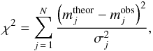 (5)where
  and
and  are the theoretical and observed magnitudes of the star at orbital phase ϕj,
  is the dispersion of the observations at orbital phase ϕj, and N the number of normal points in the curve.
The light curve solution was carried out by the following procedure. To remove the random light fluctuations, we performed preliminary averaging of the Rozhen data within the phase range of 0.01 (excluding the eclipse) for each band.
The fluxes F(ϕ) of all system components were calculated by Planck function in conditional units F(ϕ) = Fwd(ϕ) + Fred(ϕ) + Fd(ϕ) + Fhl(ϕ), and their normalization was made at phase ϕ = 0.25 of each curve by the formula m(ϕ) − m(0.25) = −2.5log [ F(ϕ) /F(0.25) ]. At the beginning of the first stage, we varied the basic system parameters freely (whose values are the same for both light curves in each filter) for each fixed value of q from the range 0.4−9.2 with step 0.1. The ranges of the basic parameters were i = 40−900, Twd = 8000−50 000 K, Tred = 2000−10 000 K, Rwd/ξ = 0.01−0.09, and Rd(max) /ξ = 0.35−0.90. By this procedure we reduced the acceptable range of q to 0.9−1.1. After that we again varied the basic parameters plus q (in the newly-obtained range) freely and obtained best solution for each curve. As a result we calculated the averaged values of the basic parameters (from their values for the all curves): q = 1.004; i = 78.8°, Rwd/ξ = 0.0227; Twd = 22 720 K. Furthermore, we fixed the basic parameters and varied the rest model parameters plus normalization parameter Fopt. Its values correspond to the same magnitudes mopt for each filter by m(ϕ) − mopt = −2.5log [ F(ϕ)) /Fopt ]. Then, Fopt was calculated as an averaged value from the two sets for each filter.
The goal of the second stage of the procedure was to search for the best solution for all eight light curves taking the normalization of the fluxes to Fopt into account for a given filter and fixed values of the basic parameters. The temperature Tred was not kept fixed because of the significant differences in its values as obtained during the first stage. The final light curve solution was obtained by varying the remaining parameters to search for the best fit ( ). The obtained parameters are given in Table 5. Figure 2 shows our synthetic light curves, the observational data, and the corresponding residuals, while Fig. 3 exhibits the geometry of the J2256 configuration.
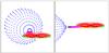 |
Fig. 3 3D configuration of J2256 at phases 0.54 (left) and 0.80 (right). Its components are shown by different colours: blue − secondary star; black point − white dwarf; red and green − inner and lateral parts of the disk; yellow − hot-spot part that is not covered by the hot line; magenta − heated part of the gas stream and black − its cold part. |
To estimate the errors of the adjusted parameters, we used the procedure described in Khruzina et al. (2013). The very small errors of the Rozhen photometric data of J2256 meant that the residuals of all obtained solutions were bigger than the critical value  . Usually, the value of the probability of rejecting the correct solution is chosen to be the level of significance α = 0.001. Thus, for our light curves with N = 68−89, we obtained
 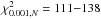 . That is why we estimated the impact of the changing of a given parameter on the solution quality. For this aim we varied each parameter around its final value until reaching (for instance) level 1.1 ( is given in Table 5), whereas all remaining parameters are kept equal to their final values. The difference between the newly obtained parameter value and its final value (Table 5) determines the corresponding error. The parameter errors obtained in this first method are given in Table 5 (the numbers in brackets).
A second, very time-consuming, approach to estimating the error of each parameter or the stability of the solution is based on arbitrary (not fixed) values of all the other parameters. For instance, to determine the precision of q one should vary the all rest parameters for each value of q (by Nelder-Mead method, see Fig. 4). The error values estimated by the second approach are an order bigger than those of the first method (for fixed rest parameters), namely: Δq ≈ 0.1, Δi ≈ 1.10, ΔRred/a0 ≈ 0.009, Δξ/a0 ≈ 0.011, ΔRwd/a0 ≈ 0.0035, ΔTwd ≈ 1500 K, and ΔTred ≈ 80 K. Usually, this second approach to estimating the parameter errors is applied for tasks with a small number of parameters or only for basic parameters.
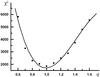 |
Fig. 4 Illustration of the q-search method for the light curve V1. |
Reproducing the observed light curves by the synthetic ones is good for the eclipses (Fig. 2), while it is acceptable for the out-of-eclipse parts. The code does not manage to describe all small features precisely, including pre-eclipse hump in B1,B2,V1. Some of these discrepancies may be attributed to the flickering that is stronger in the bluer filters, but most of them are probably result of deficiencies in our model: (i) it does not take geometric inhomogeneities of the accretion disk and possible implicit dependence of some model parameters into account; (ii) it neglects light contribution of the interstellar envelope, assuming that it has small density; (iii) the model does not take the light from the stream near L1 into account, assuming that its low temperature means low radiation in the optical range. Thus, the obtained parameter set (Table 5) should be considered as a reasonably good (but not perfect) solution to the complex multi-parametric inverse problem to reproduce numerous multi-colour data stemming from a complex multi-component configuration.
Parameters of the light curve solution of J2256 in 2013−2014.
 |
Fig. 5 Light contribution of the different energy sources of the system J2256 (in conditional units): 1 − white dwarf; 2 − normal star; 3 − accretion disk with a surface hot spot; 4 − hot line. |
Relative fluxes (in percentages) from the different emission components of J2256.
4.3. Analysis of the results
The analysis of the system parameters of J2256 (Table 5) allowed us to established which characteristics are typical of eclipsing CVs of SW Sex subtype and which are peculiar.
-
(1)
The emission of J2256 is dominated by the accretion disk withthe hot spot whose relative contributions are ~67−77%, ~69−80%, ~57−64%, and ~57−64% in the B, V, R, I bands, respectively (Table 6, Fig. 5). The biggest relative contribution of the hot spot around phases 0.7−0.85 is ~3−6%, i.e. considerably smaller than that of the disk itself. The relative contributions of the secondary star are ~10−21%, ~15−25%, ~26−32%, and ~33−37% in the B, V, R, I bands, respectively. The small (11%) contribution of the secondary in the set B1 explains the visibility of the small pre-eclipse hump on the corresponding light curve. The bigger (21%) contribution of the secondary to the curve B2 is attributed to its higher temperature. The light curve of the secondary contribution (Fig. 5) does not correspond to an ellipsoidal variability but rather to a “reflection effect” that indicates a significant heating of its surface facing to the white dwarf by the hot radiation from the disk boundary layer (Tin ~ 36 000−43 000 K). The third light contribution belongs to the hot line: biggest in the B band (~7−20%) and smallest in the I band (~6−17%). As one expects, the white dwarf makes small contribution to the emission of J2256: ~5.4%, ~3.6%, ~2.4%, and ~1.4% in filters B, V, R, and I, respectively.
-
(2)
The size of the accretion disk a/a0 ~ 0.3 (Table 5) is relatively small (Fig. 3) compared with that of the secondary component, and the disk eclipse is total. But the disk of J2256 has a relative radius Rd ~ (0.6−0.7)ξ that is similar to those of two other SW Sex stars: Rd> 0.6L1 for SW Sex (Dhillon et al. 1997) and Rd = 0.8L1 for DW UMa (Dhillon et al. 2013). The obtained value βd ~ 2−4° means that the disk of J2256 is relatively thin. The radius of the J2256 hot line near the disk is 11−28°, while the angular size of the uncovered part of the hot spot is 25−54° (Table 5).
-
(3)
The temperature Tin of the boundary layer of the disk exceeds that of the white dwarf Twd by factors of 1.5−1.7. The values of Tin in all filters are well above the standard temperatures for cataclysmic variables at quiescence (10 000−30 000 K) but are similar to those during their outbursts (Horne & Cook 1985).
- (4)
The value αg ≈ 0.5 of the parameter determining the temperature distribution along the disk radius is typical of cataclysmic variables after outbursts or in an intermediate state. The αg value of J2256 is less than that of UX UMa (0.6) but bigger than for 2MASS J01074282+4845188 (0.2). The deviation of the emission of the luminous accretion disk of J2256 from the steady-state disk emissions of NLs (with αg ≈ 0.75) may be attributed to the low viscosity of the disk matter caused by its unusually high temperature. For comparison, Rutten et al. (1992) studied accretion disks of six nova-like CVs (RW Tri, UX UMa, SW Sex, LX Ser, V1315 Aql, V363 Aur) and found that the temperatures of their disks close to the white dwarf are 10 000−30 000 K, and the temperatures of the hot spots are higher than the disk by a few thousand K. SW Sex and V1315 Aql, which are SW Sex-subtypes, exhibit a flatter temperature distribution of their disks than that of the steady-state disk (Groot et al. 2001). This result, together with our conclusions for the two SW Sex stars, 2MASS J01074282+4845188 (Khruzina et al. 2013) and J2256, imply that the non-steady-state temperature distributions of the accretion disks is an additional characteristic of the SW Sex-phenomenon.
-
(5)
The ranges in the variability of the disk parameters of J2256 in 2013−14 are: a/a0 ~ 0.27−0.33,αg ~ 0.48−0.58,Tin ~ 35 000−42 000 K. For comparison, the cataclysmic variables NZ Boo and V1239 Her show regular oscillations of the disk parameters (radius, viscosity, temperature, density) between the outbursts (steady states). Their values of αg, Tin, and βd vary notably over time even below 10 Porb, whereas the disk radii change slightly or are almost constant (Khruzina et al. 2015,b).
-
(6)
The mean temperature Twd ≈ 23 000 K of the J2256 white dwarf is in the range 19 000−50 000 K of the NLs (Warner 1995).
-
(7)
Most of the secondaries of the targets of NL, SW, UX types from the last catalogue of CVs (Ritter & Kolb 2003, update RKcat7.22, 2014) with periods in the range 0.16−0.33 d are K-type stars, but there are also M-type dwarfs (XY Ari, V373 Pup, RW Tri, UX UMa, LX Ser). The temperature of Tred ~ 3200 K of J2256 means also an M-dwarf secondary, but this value is in the range that corresponds to its binary period according to the spectral type − period relation for CVs of Knigge et al. (2011).
-
(8)
The vast majority of CVs have mass ratios that are greater than the limit q = 1.2 of a stable mass transfer of CVs (Schenker et al. 1998). The derived mass ratio of J2256 of q ~ 1.0 ± 0.1 is considerably lower. The review of the catalogue RKcat7.22 revealed two targets with small q: V363 Aur with q = 0.85 ± 0.05 and AC Cnc with q = 0.98 ± 0.04. But V363 Aur has an orbital period of 0.3212 d and a late G star as the secondary component, and AC Cnc has an orbital period of 0.3005 d and an early K star; i.e., they have quite different configurations from that of J2256. The system RW Tri seems more comparable to our target with its period of P = 0.2286 d and an early M star secondary, but its mass ratio q = 1.3 ± 0.4 cannot be considered as evidence of an exception to the rule q ≥ 1.2. Thus, the unusual combination of parameters of J2256 turned out to have no analogue amongst the known CVs.
-
(9)
The fitting of the out-of-eclipse light curves of J2256 required the emission of the hot line to be almost two times bigger at phase 0.8 than at phase 0.2 (Tables 5, 6). But this means that the temperature of its windward side is lower than that of the leeward side. This result was not expected from the theory because the numerical 3D modelling of semi-detached nonmagnetic binaries revealed that the stream from L1 causes shockless interaction with the gaseous disk at stationary outflow (Bisikalo et al. 1998; Matsuda et al. 1999; Makita et al. 2000). As a result of the interaction of the stream with the coming parts of the disk, an intensive shock wave arises at the lateral edges of the stream. Its observational appearances on the leeward stream side are equivalent to those of the hot spot on the disk. Obviously, the shock wave direction determines the higher colour temperature Tww of the matter at the windward stream part than that of its leeward side Tlw. This is true for the stationary state of the matter outflow.
The found peculiarity TIw ≥ Tww of J2256 implies non-stationary overflow from the secondary component. We have no plausible explanation of such a state during all of our observational seasons, but possible reasons could be the variable density of the gaseous stream and/or variable velocity of the outflow (owing to the highly convective envelope of the cool secondary). Some indications of this effect could be the observed narrow, blue-shifted, transient absorption features in the Balmer lines of DW UMa (Dhillon et al. 2013), which have been attributed to blobs of material ejected from the system, possibly by a magnetic propeller. Horne (1999) proposed the same explanation (magnetic propeller) on the basis of the similarity in the spectral behaviour of SW Sex stars and AE Aqr. Groot et al. (2001) went even further by considering the possibility that the SW Sex stars are intermediate polars at high inclination.
But we do not exclude the imperfections of the model as a possible reason for the J2256 peculiarity TIw ≥ Tww.
5. Analysis of the spectral data and SW Sex classification of J2256
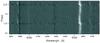 |
Fig. 6 Medium-resolution trailed spectra of J2256 covering the orbital cycle. |
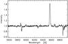 |
Fig. 7 Averaged spectrum of J2256. |
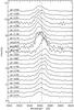 |
Fig. 8 Variability of the Hα line with the orbital phase (the laboratory wavelength is marked by a vertical dashed line). |
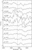 |
Fig. 9 Illustration of the variability of the HeI 5876 line with the orbital phase. |
Our medium-resolution spectra of J2256 allowed semi-quantitative analysis and led to several conclusions.
-
(a)
There are three emission lines in the observed range:Hα, HeI 5876, and HeI 6678 (Fig. 6). The Hα profiles are single-peaked (similar to those of the SW Sex-subtype stars) instead of double-peaked ones, as expected from near edge-on disks. The profiles of the HeI 5876 and HeI 6678 emission lines look double-peaked, at least at some phases (Fig. 6), but it is difficult to determine their shape for this S/N. The averaged spectrum of J2256 (Fig. 7) reveals more that the HeI 6678 line is double-peaked. We found also weak two-peaked emission lines of HeI in previous spectra of SW Sex stars: HeI 4471 and HeI 4921 of SW Sex (Dhillon et al. (1997); HeI 5785 and HeI 6678 of SW Sex at phases 0.75−0.95 (Fig. 7 in Groot et al. 2011), weak HeI lines of UU Aqr (Hoard et al. 1998), and HeI 6678 of AQ Men (Schmidtobreick et al. 2008). Dhillon et al. (1997, 2013) supposed that the dominance of the single-peaked line emission from the hot spot over the weak double-peaked disk emission leads to the strange single-peaked lines of the SW Sex-type spectra and their radial velocity curves following the motion of the bright spot. The different amplitudes of the radial velocities of the different emission lines are another confirmation of this conclusion (Tovmassian et al. 2014). The almost single-peaked emission profiles of J2256 imply considerable hot-spot contribution. However, their rotational disturbance around the mid-eclipse (Figs. 8, 9) means that part of the emission originates in the accretion disk. The secondary star successively covers the disk regions that first approaches us and then moves away from us.
-
(b)
The averaged Hα line of J2256 (Fig. 7) has an equivalent width of 29 Å. This value is less than that of SW Sex of 54 Å and close to that of DW UMa of 32 Å (Dhillon et al. 2013).
-
(c)
Both the intensity and equivalent width (EW) of the Hα line reveal phase variability (Fig. 10). The Hα and HeI 5876 emissions increase by a factor of 2 in the short phase range 0.98−0.026, i.e. at the eclipse itself. In fact, the emission lines become stronger with respect to the continuum during the eclipse because the source of continuum radiation is eclipsed (appears by the lower S/N of the spectra in Figs. 8, 9). The abrupt increase in the Hα emission at the eclipse means that the Hα emitting area is not eclipsed as strongly as the continuum emitting area; i.e., it is located above the orbital plane (Hoard et al. 2003). One can see similar behaviour during the eclipse of the Hα lines of HS 0129+2933, HS 0220+0603, and HS 0455+8513 (Rodriguez-Gil et al. 2007) as well as emission lines of UU Aqr (Hoard et al. 1998) and PG0818+513 (Thorstensen et al. 1991b). It is tempting to suppose that the increase in the emission in spectral lines at the eclipse is an additional spectral property of the SW Sex phenomenon. But we do not want to forget that at the eclipse centre itself (phase 0.00), the Hα emission seems to decrease (see Fig. 7 of PG0027+260 in Thorstensen et al. 1991a and Fig. 2 of IP Peg in Ishioka et al. 2004). Our spectra are not able to confirm the last effect because o their low time resolution. Although Fig. 10 exhibits a decrease in the Hα emission around phase 0.5, it is difficult to attribute it to the effect “phase 0.5 absorption”, which is very visible in some SW Sex stars. Absorption features of the Hβ and Hγ lines of V1315 Aql, SW Sex, and DW UMa appear in the phase range 0.4−0.7 (Szkody & Piche 1990). Thorstensen et al. (1991a) found the strong absorption at phase 0.5 for metal lines and HeI 6678 of the SW Sex star PG0027+260. The trailed spectra of HS 0220+0603 and HS 0455+8315 clearly show the effect of the “phase 0.5 absorption” of Hα, Hβ, and some HeI emission lines, but for HS 0129+2933 this effect is missing in the Balmer lines and presents in the HeI emission lines (Fig. 10, Rodriguez-Gil et al. 2007). The first deviation from the “phase 0.5 absorption” phenomenon was UU Aqr with maximum absorption in the emission lines around orbital phase 0.8 (Hoard et al. 1998). Shallow absorption dips are visible on the top of the emission Hα lines of J2256 at phases 0.7−0.9 and 0.39−0.4 (Fig. 8), which shift in phase with the wide emission profiles but with considerably lower radial velocity. These dips are rather individual peaks of the different emission sources than some appearances of the “phase 0.5 absorption” effect.
-
(d)
The trailed spectra (Fig. 6) reveal that the Hα and HeI 5876 emission lines of J2256 reveal S-wave wavelength shifts. However, the smooth Doppler shifts of these lines are disturbed by jumps (discontinuities) to the shorter wavelength around phase 0.0 (Figs. 6, 8, 9). The jump of the Hα line amounts to more than 10 Å while that of HeI 5876 seems bigger. The Doppler jumps of the Hα line around phase 0.0 were also observed for other SW Sex stars (Fig. 9 in Rodriguez-Gil et al. 2007; Fig. 4 in Tovmassian et al. 2014), as well as for the lines Hβ and HeII 4686 of the eclipsing dwarf nova IP Peg (Ishioka et al. 2004). Our medium-resolution spectra allow approximate estimations of the radial velocities during the orbital cycle. For this aim we fitted the Hα lines of J2256 by Gausians (Thorstensen 2000). Excluding the several outliers around phase 0.0, we obtained semi-amplitude of the radial velocities of the emitting material 210 ± 50 km s-1 (Fig. 11), a typical value for SW Sex type stars. The γ velocity of J2256 is −85 km s-1.
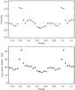
Fig. 10 Phase variability of the intensity and EW of the Hα line.
-
(e)
There is a phase discrepancy of ~0.03 between the photometric and spectral data of J2256 that is a typical property of the SW Sex stars.
-
(f)
The different widths of the emission lines of J2256 (Fig. 6) mean that they originate in different disk regions with different velocities and different temperatures.
-
(g)
The absence of total disappearance of the emission lines of J2256 means that they are formed above the disk and probably originate in a vertically extended hot-spot halo.
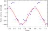
Fig. 11 Variability in the radial velocities according to the measurement of the Hα profiles.
The analysis of our medium-resolution spectra revealed that J2256 posses all spectral characteristics of the SW Sex subtype of the cataclysmic variables (defined by Thorstensen 1991, Rodriguez-Gil et al. 2007; Schmidtobreick et al. 2009) apart from the 0.5 central absorption. The value Porb = 5.5 h of J2256 is slightly higher than the period range 3.0−4.5 h of the known SW Sex stars, most of them tightly clustered just above the period gap of CVs (Rodriguez-Gil et al. 2007). But there are members with considerably longer periods (Bisol et al. 2012; Khruzina et al. 2013).
6. Conclusions
The main results of the prolonged observations of the newly discovered cataclysmic variable J2256, and their modelling and analysis led to the following conclusions.
-
1.
J2256 shows the deepest eclipse among the known eclipsing nova-like variables.
-
2.
The BVRI light curves of the target were reproduced well by a configuration consisting of a red dwarf and a white dwarf that is surrounded by an accretion disk with a hot spot and a hot line.
-
3.
The observed deep minimum of J2256 was reproduced by the eclipse of a very bright, thin, small, but hot accretion disk. The high temperature of its inner regions of ~38 000−41 000 K is typical of cataclysmic variables during outburst.
-
4.
The temperature distribution along the disk is flatter than that of steady-state disk, which is typical of NLs. It was supposed that the non-steady-state temperature distributions of the accretion disks is an additional brand of the SW Sex-phenomenon.
-
5.
The white dwarf of J2256 has a temperature around 22 000 K, while the secondary star is an M dwarf.
-
6.
The derived mass ratio of J2256 of q ~ 1.0 ± 0.1 is considerably lower than the limit q = 1.2 of the stable mass transfer of CVs. The combination of the period, mass ratio, and secondary temperature of J2256 turned out not to have an analogue amongst the known CVs.
-
7.
The radiation of J2256 in the visual spectral range is dominated by the emission of the accretion disk, whose relative contribution is around 70%, followed by that of the secondary star (around 20%) and hot line (around 10%).
-
8.
We found an unusual temperature distribution of the hot line of J2256: the temperature of its windward side is lower than that of the leeward side.
-
9.
The emission of J2256 in the lines Hα, HeI 5875, and HeI 6678 increases considerably (twice) around the eclipse centre. This effect is accompanied by large Doppler jumps of these lines. The absence of eclipses of the emission lines and their single-peaked profiles means that they originate mainly in a vertically extended hot-spot halo.
-
10.
The emission Hα line reveals S-wave wavelength shifts with semi-amplitude of around 210 km s-1 and phase lag of 0.03.
-
11.
J2256 does not exhibit “phase 0.5 absorption” phenomena, which are assumed to be a characteristic of the SW Sex stars.
Acknowledgments
This study is supported by funds of the projects: RD 08-285/2015 of Shumen University, grant 14-02-00825 of the Russian Foundation for fundamental Research and NSh-1675.2014.2 of the Programme of State Support to Leading Scientific Schools. D.K. and D.D. gratefully acknowledge observing grant support from the Institute of Astronomy and Rozhen National Astronomical Observatory, Bulgarian Academy of Sciences. The authors are very grateful to the anonymous referee for the valuable notes, advice, and suggestions. This publication makes use of data products from the Two Micron All Sky Survey, which is a joint project of the University of Massachusetts and the Infrared Processing and Analysis Center/California Institute of Technology, funded by the National Aeronautics and Space Administration and the National Science Foundation (Skrutskie et al. 2006). We have used also “The Guide Star Catalogue, Version 2.3.2” (Lasker et al. 2008) and “The USNO-B Catalog” (Monet et al. 2003). This research makes use of the SIMBAD and Vizier data bases, operated at the CDS, Strasbourg, France, and the NASA Astrophysics Data System Abstract Service. The software Table curve 2D is product of Systat Software, Inc. (info-usa@systat.com, Corporate Headquarters).
References
- Ballouz, R., Sion, E. M., & 2009, ApJ, 697, 1717 [NASA ADS] [CrossRef] [Google Scholar]
- Bisikalo, D. V., Boyarchuk, A. A., Chechetkin, V. M., et al. 1998, MNRAS, 390, 39 [NASA ADS] [CrossRef] [Google Scholar]
- Bisol, A. C., Godon, P., & Sion, E. M. 2012, PASP, 124, 158 [NASA ADS] [CrossRef] [Google Scholar]
- Casares, J., Martinez-Pais, I. G., Marsh, T. R., Charles, P. A., & Lazaro, C. 1996, MNRAS, 278, 219 [NASA ADS] [CrossRef] [Google Scholar]
- Dhillon, V. S., Marsh, T. R., Jones, D. H. P. & 1997, MNRAS, 291, 694 [NASA ADS] [CrossRef] [Google Scholar]
- Dhillon, V. S., Smith, D. A., & Marsh, T. R. 2013, MNRAS, 428, 3559 [NASA ADS] [CrossRef] [Google Scholar]
- Dimitrov, D., & Kjurkchieva, D. 2012, New Astron., 17, 34 [NASA ADS] [CrossRef] [Google Scholar]
- Groebel, R. 2009, BAVSR, 58, 80 [NASA ADS] [Google Scholar]
- Groot, P. J., Rutten, R. G. M., & van Paradijs, J. 2001, A&A, 368, 183 [NASA ADS] [CrossRef] [EDP Sciences] [Google Scholar]
- Hellier, C. 2001, Cataclysmic Variable Stars − How and Why They Vary (Springer Praxis books in Astronomy and Space Sciences) [Google Scholar]
- Hellier, C., & Robinson, E. L. 1994, ApJ, 431, L107 [NASA ADS] [CrossRef] [Google Scholar]
- Hoard, D. W., Szkody, P., Froning, C. S., Long, K. S., & Knigge, C. 2003, AJ, 126, 2473 [NASA ADS] [CrossRef] [Google Scholar]
- Hoard, D. W., Szkody, P., Still, M. D., Smith, R. C., & Buckley, D. A. H. 1998, MNRAS, 294, 689 [NASA ADS] [CrossRef] [Google Scholar]
- Horne, K., & Cook, M. C. 1985, MNRAS, 214, 307 [NASA ADS] [Google Scholar]
- Horne, K., & Marsh, T. 1986, MNRAS, 218, 761 [NASA ADS] [CrossRef] [Google Scholar]
- Horne, K. 1999, ASP Conf. Ser., 157, 349 [NASA ADS] [Google Scholar]
- Howell, S. B., Nelson, L. A., & Rappaport, S. 2001, ApJ, 550, 897 [NASA ADS] [CrossRef] [Google Scholar]
- Ishioka, R., Mineshige, S., Kato, T., Nogami, D., & Uemura, M. 2004, PASJ, 56, 481 [NASA ADS] [Google Scholar]
- Khruzina, T. S. 1998, Astron. Rep., 42, 180 [NASA ADS] [Google Scholar]
- Khruzina, T. S. 2011, Astron. Rep., 55, 425 [NASA ADS] [CrossRef] [Google Scholar]
- Khruzina, T. S., Cherepashchuk, A. M., Bisikalo, D. V., Boyarchuk, A. A., & Kuznetsov, O. A. 2003, Astron. Rep., 47, 214 [NASA ADS] [CrossRef] [Google Scholar]
- Khruzina, T., Dimitrov, D., & Kjurkchieva, D. 2013, A&A, 551, A125 [NASA ADS] [CrossRef] [EDP Sciences] [Google Scholar]
- Khruzina, T. S., Golysheva, P., Katysheva, N., Shugarov, S., & Shakura, N. I. 2015, Astron. Rep., 59, 288 [NASA ADS] [CrossRef] [Google Scholar]
- Knigge, C., Long, K. S., Hoard, D. W., Szkody, P., & Dhillon, V. S. 2000, ApJ, 539, L49 [NASA ADS] [CrossRef] [Google Scholar]
- Knigge, C., Baraffe, I., & Patterson, J. 2011, ApJS, 194, 28 [NASA ADS] [CrossRef] [Google Scholar]
- Kwee, K. K., & van Woerden, H. 1956, Bull. Astron. Inst. Neth., 9, 252 [Google Scholar]
- Lasker, B., Lattanzi, M. G., McLean, B. J., et al. 2008, AJ, 136, 735 [NASA ADS] [CrossRef] [PubMed] [Google Scholar]
- Makita, M., Miyawaki, K., & Matsuda, T. 2000, MNRAS, 316, 906 [NASA ADS] [CrossRef] [Google Scholar]
- Matsuda, T., Makita, M., & Boffin, H. M. J. 1999, Proc. of the Disk Instabilities in Close Binary Systems, October 27−30, 1998, Kioto, Japan/eds. S. Mineshige, & J. C. Wheeler (Tokio, Japan: Universal Acad. Press), 129 [Google Scholar]
- Monet, D. G., Levine, S. E., Casian, B., et al. 2003, AJ, 125, 984 [NASA ADS] [CrossRef] [Google Scholar]
- Motl, D. 2012, http://sourceforge.net/projects/c-munipack/files/ [Google Scholar]
- Neustroev, V. V., Suleimanov, V. F., Borisov, N. V., Belyakov, K. V., & Shearer, A. 2011, MNRAS, 410, 963 [NASA ADS] [CrossRef] [Google Scholar]
- Noebauer, U. M., Long, K. S., Sim, S. A., & Knigge, C. 2010, ApJ, 719, 1932 [NASA ADS] [CrossRef] [Google Scholar]
- Osaki, Y. 2005, Proc. Jpn. Acad. Ser. B, 81, 291 [NASA ADS] [CrossRef] [Google Scholar]
- Osterbrock, D. E., Fulbright, J. P., Martel, A. R., et al. 1996, PASP, 108, 277 [NASA ADS] [CrossRef] [Google Scholar]
- Papadaki, C., Boffin, H. M. J., Stanishev, V., et al. 2009, JAD, 15, 1 [NASA ADS] [Google Scholar]
- Press, W. H., Flannery, B. P., Teukolsky, S. A. 1986, Numerical recipes. The Art of Scientific Computing (Cambridge Univ. Press) [Google Scholar]
- Ritter, H., & Kolb, U. 2003, A&A, 404, 301 [NASA ADS] [CrossRef] [EDP Sciences] [Google Scholar]
- Rodriguez-Gil, P., Gansicke, B. T., Hagen, H. J., et al. 2007, MNRAS, 377, 1747 [NASA ADS] [CrossRef] [Google Scholar]
- Rutten, R. G. M., van Paradijs, J., & Tinbergen, J. 1992, A & A, 260, 213 [Google Scholar]
- Schenker, K., Kolb, U., & Ritter, H. 1998, MNRAS, 297, 633 [NASA ADS] [CrossRef] [Google Scholar]
- Schmidtobreick, L., Pablo, R. G., & Boris, T. G. 2008, Mem. S. A. It. 75, 282 [Google Scholar]
- Schmidtobreick, L., Rodriguez-Gil, P., & Gansicke, B. 2009, Rev. Mex. Astron. Astrofis. Conf. Ser., 35, 115 [NASA ADS] [Google Scholar]
- Skrutskie, M. F., Cutri, R. M., Stiening, R., et al. 2006, AJ, 131, 1163 [NASA ADS] [CrossRef] [Google Scholar]
- Stanishev, V., Kraicheva, Z., Boffin, H. M. J., et al. 2004, A&A, 416, 1057 [NASA ADS] [CrossRef] [EDP Sciences] [Google Scholar]
- Szkody, P., & Piche, F. 1990, ApJ, 361, 235 [NASA ADS] [CrossRef] [Google Scholar]
- Thorstensen, J. R. 2000, PASP, 112, 1269 [NASA ADS] [CrossRef] [Google Scholar]
- Thorstensen, J. R., Ringwald, F. A., Wade, R. A., Schmidt, G. D., & Norsworthy, J. E. 1991a, AJ, 102, 272 [NASA ADS] [CrossRef] [Google Scholar]
- Thorstensen, J. R., Davis, M. K., & Ringwald, F. A. 1991b, AJ, 102, 683 [NASA ADS] [CrossRef] [Google Scholar]
- Tovmassian, G., Stephania Hernandez, M., Gonzalez-Buitrago, D., Zharikov, S., & Garcia-Diaz, M. 2014, AJ, 147, 68 [NASA ADS] [CrossRef] [Google Scholar]
- Townsley, D. M., & Bildsten, L. 2003, ApJ, 596, L227 [NASA ADS] [CrossRef] [Google Scholar]
- Townsley, D. M., & Gansicke, B. T. 2009, ApJ, 693, 1007 [NASA ADS] [CrossRef] [Google Scholar]
- Warner, B. 1995, Cataclysmic Variable Stars, Cambridge Astrophys. Ser., 28 [Google Scholar]
- Williams, R. E. 1989, AJ, 97, 1752 [NASA ADS] [CrossRef] [Google Scholar]
- Witham, A. R., Knigge, C., Drew, J. E., et al. 2008, MNRAS, 384, 1277 [NASA ADS] [CrossRef] [Google Scholar]
All Tables
Coordinates and magnitudes of the comparison stars for the data of the 60 cm telescope.
Relative fluxes (in percentages) from the different emission components of J2256.
All Figures
|
Fig. 1 Representative (annual) samples of the numerous Nürnberg unfiltered light curves of J2256 during 2008−2014 (the symbol sizes correspond to the photometric error of around 0.02 mag). |
| In the text | |
|
Fig. 2 a) Rozhen photometric data of J2256 (points with the corresponding error bars), the synthetic light curves (continuous lines), and the corresponding residuals; b) details around the eclipse minima (the error bars are smaller than the symbol size); c) details of the out-of-eclipse parts of light curves. |
| In the text | |
|
Fig. 3 3D configuration of J2256 at phases 0.54 (left) and 0.80 (right). Its components are shown by different colours: blue − secondary star; black point − white dwarf; red and green − inner and lateral parts of the disk; yellow − hot-spot part that is not covered by the hot line; magenta − heated part of the gas stream and black − its cold part. |
| In the text | |
|
Fig. 4 Illustration of the q-search method for the light curve V1. |
| In the text | |
|
Fig. 5 Light contribution of the different energy sources of the system J2256 (in conditional units): 1 − white dwarf; 2 − normal star; 3 − accretion disk with a surface hot spot; 4 − hot line. |
| In the text | |
|
Fig. 6 Medium-resolution trailed spectra of J2256 covering the orbital cycle. |
| In the text | |
|
Fig. 7 Averaged spectrum of J2256. |
| In the text | |
|
Fig. 8 Variability of the Hα line with the orbital phase (the laboratory wavelength is marked by a vertical dashed line). |
| In the text | |
|
Fig. 9 Illustration of the variability of the HeI 5876 line with the orbital phase. |
| In the text | |
|
Fig. 10 Phase variability of the intensity and EW of the Hα line. |
| In the text | |
|
Fig. 11 Variability in the radial velocities according to the measurement of the Hα profiles. |
| In the text | |
Current usage metrics show cumulative count of Article Views (full-text article views including HTML views, PDF and ePub downloads, according to the available data) and Abstracts Views on Vision4Press platform.
Data correspond to usage on the plateform after 2015. The current usage metrics is available 48-96 hours after online publication and is updated daily on week days.
Initial download of the metrics may take a while.