| Issue |
A&A
Volume 583, November 2015
|
|
|---|---|---|
| Article Number | A62 | |
| Number of page(s) | 14 | |
| Section | Stellar structure and evolution | |
| DOI | https://doi.org/10.1051/0004-6361/201526390 | |
| Published online | 28 October 2015 | |
Using seismic inversions to obtain an indicator of internal mixing processes in main-sequence solar-like stars
1 Institut d’Astrophysique et Géophysique de l’Université de Liège, Allée du 6 août 17, 4000 Liège, Belgium
e-mail: This email address is being protected from spambots. You need JavaScript enabled to view it.
2 School of Physics and Astronomy, University of Birmingham, Edgbaston, Birmingham, B15 2TT, UK
Received: 23 April 2015
Accepted: 16 July 2015
Abstract
Context. Currently, seismic modelling is one of the best ways of building accurate stellar models, thereby providing accurate ages. However, current methods are affected by simplifying assumptions concerning stellar mixing processes. In this context, providing new structural indicators that are less model-dependent and more sensitive to mixing processes is crucial.
Aims. We wish to build a new indicator for core conditions (i.e. mixing processes and evolutionary stage) on the main sequence. This indicator tu should be more sensitive to structural differences and applicable to older stars than the indicator t presented in a previous paper. We also wish to analyse the importance of the number and type of modes for the inversion, as well as the impact of various constraints and levels of accuracy in the forward modelling process that is used to obtain reference models for the inversion.
Methods. First, we present a method of obtaining new structural kernels in the context of asteroseismology. We then use these new kernels to build a new indicator of central conditions in stars, denoted tu, and test it for various effects including atomic diffusion, various initial helium abundances, and various metallicities, following the seismic inversion method presented in our previous paper. We then study the indicator’s accuracy for seven different pulsation spectra including those of 16CygA and 16CygB and analyse how it depends on the reference model by using different constraints and levels of accuracy for its selection.
Results. We observe that the inversion of the new indicator tu using the SOLA method provides a good diagnostic for additional mixing processes in central regions of stars. Its sensitivity allows us to test for diffusive processes and chemical composition mismatch. We also observe that using modes of degree 3 can improve the accuracy of the results, as well as using modes of low radial order. Moreover, we note that individual frequency combinations should be considered to optimise the accuracy of the results.
Key words: stars: interiors / stars: oscillations / asteroseismology / stars: fundamental parameters
© ESO, 2015
1. Introduction
Determining accurate and precise stellar ages is a major problem in astrophysics. These determinations are either obtained through empirical relations or model-dependent approaches. Moreover, accurate stellar ages are crucial when studying stellar evolution, when determining properties of exoplanetary systems or when characterising stellar populations in the galaxy. However, the absence of a direct observational method for measuring this quantity makes such determinations rather complicated. Age is usually related empirically to the evolutionary stage or determined through model dependent techniques like the forward asteroseismic modelling of stars. However, this model-dependence is problematic because, if a physical process is not taken into account during the modelling, it will introduce a bias when determining the age, as well as in the determination of other fundamental characteristics like the mass or the radius (see, for example, Eggenberger et al. 2010, for the impact of rotation on asteroseismic properties, and Miglio et al. 2015, for a discussion in the context of ensemble asteroseismology, and Brown et al. 1994, for a comprehensive study of the relation between seismic constraints and stellar model parameters). It is also clear that asteroseismology probes the evolutionary stage of stars and not the age directly. In other words, we are able to analyse the stellar physical conditions but relating these properties to an age will, ultimately, always depend on assumptions made during the building of the evolutionary sequence of the model. A general review of the impact of the hypotheses of stellar modelling and of asteroseismic constraints on the determination of stellar ages is presented in Lebreton et al. (2014a) and Lebreton et al. (2014b).
In the sense of this age determination problematic, the question of additional mixing processes is central (Dupret 2008) and can only be solved by using less model dependent seismic analysis techniques and new generations of stellar models. These new seismic methods should be able to provide relevant constraints on the physical conditions in the central regions and help with the inclusion of additional mixing in the models. In this context, seismic inversion techniques are an interesting way to relate structural differences to frequency differences and therefore offer a new insight into the physical conditions inside observed stars. From the observational point of view, the high quality of the Kepler and CoRoT data as well as the selection of the Plato mission (Rauer et al. 2014) allows us to expect enough observational data to carry out inversions of global characteristics. In the context of helioseismology, structural inversion techniques have already led to noteworthy successes. They have provided strong constraints on solar atomic diffusion (see Basu et al. 1996b), thus confirming the work of Elsworth et al. (1990). However, application of structural inversion techniques in asteroseismology is still limited. Inversions for rotation profiles have been carried out (see for example Deheuvels et al. 2014, for an application to Kepler subgiants), but as far as structural inversions are concerned, one can use either non-linear (see Roxburgh 2010, 2015, for an example of the differential response technique), or linear inversion techniques applied to integrated quantities as in Reese et al. (2012) and Buldgen et al. (2015).
In our previous paper (see Buldgen et al. 2015), we extended mean density inversions based on the SOLA technique (Reese et al. 2012) to inversions of the acoustic radius of the star and an indicator of core conditions, denoted t. We also developed a general approach to determining custom-made global characteristics for an observed star. We showed that applying the SOLA inversion technique (Pijpers & Thompson 1994) to a carefully selected reference model, obtained via the forward-modelling technique, could lead to very accurate results. However, it was then clear that the first age indicator was limited to rather young stars and that other indicators should be developed. Moreover, the model dependence of these techniques should be carefully studied and there is a need to define a more extended theoretical background for these methods. The influence of the number but also the type of modes used for a specific inversion should be investigated. In the end, one should be able to define whether the inversion should be carried out or not, knowing the number of observed frequencies and the quality of the reference model according to its selection criteria.
In this study, we offer an answer to these questions and provide a new indicator for the mixing processes and the evolutionary stage of an observed star. We structure our study as follows: Sect. 2 introduces a technique to obtain equations for new structural kernels in the context of asteroseismology and applies it to the (u,Γ1) and the (u,Y) kernels, where u is the squared isothermal sound speed, Γ1 the adiabatic gradient and Y the current helium abundance profile. Section 3 introduces a new indicator of mixing processes and evolutionary stages, which is not restricted to young stars, as was the case for the indicator presented in Buldgen et al. (2015). Having introduced this new indicator, we test its accuracy using different physical effects such as including atomic diffusion processes with high velocities (up to 2.0 times the solar microscopic diffusion velocities) in the target, changing the helium abundance, changing the metallicity and changing the solar mixture of heavy elements. Section 4 analyses the impact of the type and number of modes on the inversion results whereas Sect. 5 studies how the accuracy depends on the reference model. We also tested our method on targets similar to the binary system 16CygA and 16CygB using the same modes as those observed in Verma et al. (2014) to show that our method is indeed applicable to current observational data. Section 6 summarises our results and presents some prospects on future research for global quantities that could be obtained with the SOLA inversion technique.
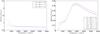 |
Fig. 1 Verification of Eq. (1) for a set of 120 modes with the · being the 40 radial modes, the × being the 40 dipolar modes and the + being the 40 quadrupolar modes. The left plot illustrates this verification for the (ρ,c2) couple when no scaling is applied to c2 whereas the right plot illustrates the same verification for the (ρ,c2) couple when scaling is applied to c2, as well as the (ρ,Γ1) couple where no scaling is needed. |
2. (u,Γ1) and (u,Y) structural kernels
2.1. Integral equations for structural couples in the asteroseismic context
Gough & Thompson (1991) demonstrated that one could deduce a linear integral relation between the perturbations of frequencies and the perturbation of structural variables from the variational principle. This equation is obtained by assuming the adiabatic approximation and spherical symmetry, and by neglecting surface integral terms. It is only valid if the stellar models are close to each other. If one is working with the structural pair (c2,ρ), where c2 is the adiabatic squared sound velocity and ρ the density, this relation takes on the form:  (1)where
  with R the stellar radius, and where the classical definition of the relative differences between the target and model for any structural quantity s has been used:
  (2)In what follows, we always use the subscript or superscript “obs” when referring to the observed star, “ref” for the reference model variables in perturbation definitions, and “inv” for inverted results. Other variables, like the kernel functions, which are denoted without subscripts or superscripts, are of course related to the reference model and are known in practice. Finally, one should also note that the suffix i is only meant to be an index to classify the modes. Moreover, since it is clear that some hypotheses are not suitable for surface regions, a supplementary function,
  was added to model these so-called surface effects. It is defined as a linear combination of Legendre polynomials, normalised by the factor Qi, which is the mode inertia normalised by the inertia of a radial mode interpolated to the same frequency. We emphasise here that neither this normalisation coefficient nor the treatment of surface effects are uniquely defined and that other techniques have also been used (see for example Dziembowski et al. 1990; Däppen et al. 1991; Basu et al. 1996a).
The kernels of the couple (ρ,Γ1) have already been presented in Gough & Thompson (1991) who also mentionned the use of another method, defined in Masters (1979) to modify Eq. (1) and obtain such relations for the (c2,Γ1) couple and also the (N2,c2) couple. Other approaches to obtaining new structural kernels were presented (see for example Elliott 1996; Kosovichev 1999, for the application of the adjoint equations method to this problem). The latter approach has been used in helioseismology where it was assumed that the mass of the observed star is known to a sufficient level of accuracy to impose surface boundary conditions. In the context of asteroseismology, we cannot make this assumption. Nevertheless, the approach defined in Masters (1979) allows us to find ordinary differential equations for a large number of supplementary structural kernels, without assuming a fixed mass1.
Another question arises in the context of asteroseismology: what about the radius? We implicitly define our integral equation in non-dimensional variables but how do we relate the structural functions, for example  defined for the observed star and
  defined for the reference model? What are the implications of defining all functions in the same domain in
  varying from 0 to 1? It was shown by Basu (2003) that an implicit scaling was applied by the inversion in the asteroseismic context. The observed target is homologously rescaled to the radius of the reference model, while its mean density is preserved. This means that the oscillation frequencies are the same, but other quantities such as the adiabatic sound speed c, and the squared isothermal sound speed
  , will be rescaled. Therefore, when inverted, they are not related to the real target but to a scaled one.
This can be demonstrated with the following simple test. We can take two models a few time steps from one another on the same evolutionary sequence knowing that they should not be that different. (Here, we consider 1 M⊙, main-sequence models.) We then test the verification of Eq. (1) by plotting the following relative difference  (3)with
  defined as
 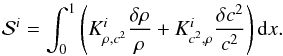 (4)The results are plotted in blue in the left panel of Fig. 1, where we can see that this equation is not satisfied. However, one might think that this inaccuracy is related to the neglected surface terms or to non-linear effects. Therefore we carry out the same test using the (ρ,Γ1) kernels, plotted in red in the right-hand panel of Fig. 1. We see that for these kernels, the equation is satisfied. Moreover, when separating the contributions of each structural term, we see that the errors arise from the term related to c2 in the first case. Using the scaled adiabatic sound speed, however, leads to the blue symbols in the right-hand panel of Fig. 1 and we directly see that in this case, the integral equation is satisfied. This leads to the conclusion that inversion results based on integral equations are always related to the scaled target and not the target itself, as concluded by Basu (2003). We see in Sect. 3 that this has strong implications for the structural information given by inversion techniques.
2.2. Differential equation for the (u, Γ1) and the (u, Y) kernels
As mentioned in the previous section, the method described in Masters (1979) allows us to derive differential equations for structural kernels. In what follows, we will apply this method to the (u,Γ1) and the (u,Y) kernels. However, this approach can be applied to many other structural pairs such as: (c2,Γ1), (c2,Y), (g,Γ1), (g,Y), ..., with  the squared adiabatic sound speed,
  the local gravity,
  the adiabatic exponent and Y the local helium abundance. We do not describe these kernels since they are straightforward to obtain using the same technique as that which will be used here for the (u,Γ1) kernels. One should also note that a differential equation cannot be obtained for the couple (N2,c2), with N2 the Brunt-Väisälä frequency, defined as:
  , without neglecting a supplementary surface term.
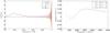 |
Fig. 2 Left: plot illustrating the verification of Eq. (10) for n = 15, ℓ = 0 kernel K15,0, where ℐu,Γ1 is the right-hand side of this equation and ℛ is the residual. Right: same test as in Fig. 1 for the (u,Γ1) kernels. |
The first step is to assume that if these kernels exist, they should satisfy an integral equation of the type given in Eq. (1), thereby leading to: 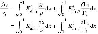 (5)From that point, we use the definition of u to express the first integral in terms of a density perturbation. This is done using the definition of the pressure, P, and the cumulative mass up to a radial position, r:
 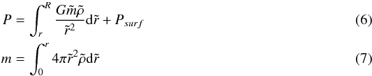 where we neglect the pressure perturbation at the surface. In what follows, we use the non-dimensional forms
  , where M is the stellar mass, R the stellar radius and G the gravitational constant,
  and
and  . To avoid any confusion in already rather intricate equations, we drop the hat notation in what follows and denote these non-dimensional variables P, m and ρ. Using Eqs. (6) and (7), one can relate u perturbations to P and ρ perturbations as
  (8)However, using Eq. (6), one can also relate P perturbations to ρ perturbations. Doing this, one should note that the surface pressure perturbation is usually neglected and considered as a so-called surface effect. Using non-dimensional variables and combining Eqs. (6) and (7) in Eq. (8), one obtains an expression relating u perturbations solely to ρ perturbations. (Of course, this is an integral relation due to the definition of the hydrostatic pressure, P). One can use this relation to replace
  in Eq. (5) and after the permutation of the integrals stemming from the definition of the hydrostatic pressure perturbation, one obtains the following integral equation relating
  to
to  :
: ![Mathematical equation: \begin{eqnarray} \int_{0}^{1}K^{i}_{\rho,\Gamma_{1}} && \frac{\delta \rho}{\rho}{\rm d}x + \int_{0}^{1}K^{i}_{\Gamma_{1},\rho}\frac{\delta \Gamma_{1}}{\Gamma_{1}}{\rm d}x = \int_{0}^{1}\left(\frac{m(x)\rho}{x^{2}}\left[\int_{0}^{x}\frac{K^{i}_{u,\Gamma_{1}}}{\bar{P}}{\rm d}\bar{x}\right] \right. \nonumber \\ && \left. +4 \pi x^{2} \rho\left[\int_{x}^{1} \frac{\tilde{\rho}}{\tilde{x}^{2}} \left[\int_{0}^{\tilde{x}}\frac{K^{i}_{u,\Gamma_{1}}}{\bar{P}} {\rm d}\bar{x} \right] {\rm d}\tilde{x} \right] -K^{i}_{u,\Gamma_{1}}\right) \frac{\delta \rho}{\rho} {\rm d}x \nonumber \\ &&+ \int_{0}^{1}K^{i}_{\Gamma_{1},u}\frac{\delta \Gamma_{1}}{\Gamma_{1}}{\rm d}x. \end{eqnarray}](/articles/aa/full_html/2015/11/aa26390-15/aa26390-15-eq75.png) (9)One should be careful when solving this equation since one is faced with multiple integrals, with certain equilibrium variables associated to
(9)One should be careful when solving this equation since one is faced with multiple integrals, with certain equilibrium variables associated to  or
or  . Therefore care should be taken when integrating to check the quality of the result. To obtain a differential equation, we note that it is clear that the equation is satisfied if the integrands are equal, meaning that the kernels are related as follows:
 ![Mathematical equation: \begin{eqnarray} K^{i}_{\rho,\Gamma_{1}}&=\,& \frac{m(x)\rho}{x^{2}}\left[\int_{0}^{x}\frac{K^{i}_{u,\Gamma_{1}}}{\bar{P}}{\rm d}\bar{x}\right] \nonumber \\ && +4 \pi x^{2} \rho\left[\int_{x}^{1} \frac{\tilde{\rho}}{\tilde{x}^{2}} \left[\int_{0}^{\tilde{x}}\frac{K^{i}_{u,\Gamma_{1}}}{\bar{P}} {\rm d}\bar{x} \right] {\rm d}\tilde{x} \right] -K^{i}_{u,\Gamma_{1}}, \label{eqkernelugamma} \\ K^{i}_{\Gamma_{1},\rho} &=\,& K^{i}_{\Gamma_{1},u}. \label{eqkernelgammau} \end{eqnarray}](/articles/aa/full_html/2015/11/aa26390-15/aa26390-15-eq78.png) Given this integral expression, one can simply derive and simplify the expression to obtain a second-order ordinary differential equation in x as follows:
Given this integral expression, one can simply derive and simplify the expression to obtain a second-order ordinary differential equation in x as follows: ![Mathematical equation: \begin{eqnarray} -y\frac{{\rm d}^{2}\kappa^{'}}{({\rm d}y)^{2}}&+&\left[\frac{2 \pi y^{3/2}\tilde{\rho}}{\tilde{m}}-3 \right]\frac{{\rm d} \kappa^{'}}{{\rm d}y}=y\frac{{\rm d}^{2} \kappa}{({\rm d}y)^{2}} \nonumber\\ &-&\left[\frac{2 \pi y^{3/2} \tilde{\rho}}{\tilde{m}}-3 +\frac{\tilde{m} \tilde{\rho}}{2 y^{1/2} \tilde{P}} \right]\frac{{\rm d} \kappa}{{\rm d}y} \nonumber\\ &+& \left[\frac{\tilde{m} \tilde{\rho}}{4 y \tilde{P}^{2}} \frac{{\rm d}\tilde{P}}{{\rm d}x} - \frac{\tilde{m}}{4y \tilde{P}} \frac{{\rm d} \tilde{\rho}}{{\rm d}x}-\frac{3}{4y^{1/2} \tilde{P}}\frac{{\rm d}\tilde{P}}{{\rm d}x} -\frac{\tilde{m} \tilde{\rho}}{2y^{3/2}\tilde{P}}\right] \kappa, \label{eqdiffugamma} \end{eqnarray}](/articles/aa/full_html/2015/11/aa26390-15/aa26390-15-eq80.png) (12)where
(12)where  ,
,  and y = x2. The central boundary condition in terms of κ and κ′ is obtained by taking the limit of Eq. (12) as y goes to 0. The additional boundary conditions are obtained from Eq. (10). Namely, we impose that the solution satisfies Eq. (10) at some point of the domain. This system is then discretised using a finite difference scheme based on Reese (2013), and solved using a direct band-matrix solver.
Two quality checks can be made to validate our solution, the first being that every kernel satisfies Eq. (10), the second being that they satisfy a frequency-structure relation (as in Eq. (5)) within the same accuracy as the classical structural kernels (ρ,Γ1) or (ρ,c2). We can carry out the same analysis as in Sect. 2.1, keeping in mind that the squared isothermal sound speed will also be implicitly rescaled by the inversion since it is proportional to  , as is the squared adiabatic sound speed, c2. The results of this test are plotted in Fig. 2 along with an example of the verification of the integral equation for the kernel associated with the ℓ = 0, n = 15 mode.
 |
Fig. 4 Structural kernels for the n = 15, ℓ = 0 mode associated with the (u,Γ1) couple on the left hand side and with the (u,Y) couple on the right hand side. |
The equation for the (u,Y) kernels is identical when using the following relation: 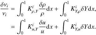 (13)meaning that Eq. (12) can simply be transposed using the definitions:
  and
and  . One could also start from Eq. (5), use the definition:
 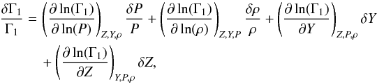 (14)and neglect the δZ contribution. This assumption is particularly justified if one places spectroscopic constraints on the metallicity. Nevertheless, the term associated with δZ is smaller than the three other terms and if one is probing the core regions, the
  contribution is already very small. Consequently, all of the terms of Eq. (14) are small compared to the integral contribution. Still, this assumption is not completely sound if one wishes to probe surface regions. When comparing the
  to the
  , we notice that their amplitude is comparable and that is even often larger. However, we have to consider that it will be multiplied by δZ, which is much smaller than δY. Moreover, the functions are somewhat alike in central regions and, as a consequence, there will be an implicit partial damping of the δZ term when damping the δY contribution if it is in the cross-term of the inversion. We can control the importance of this assumption by switching from the (u,Y) kernels to the (u,Γ1) kernels. Indeed, if the error is large, the inversion result will be changed by the contribution from the neglected term. In conclusion, in the case of the inversion of tu, we present and use in the next sections, this assumption is justified, but this is not certain for inversions of helium mass fraction in upper layers, for which only numerical tests for the chosen indicator will provide a definitive answer.
 |
Fig. 5 Left panel: structural changes in the scaled |


Knowing these facts, we can search for the (u,Y) kernels using the previous developments. It is in fact straightforward when using the (ρ,Y) kernels, which are directly obtained from (ρ,Γ1) or (ρ,c2). However, one should also note that by using Eq. (14), we assume that the equation of state is known for the target which might introduce small errors2. Again, Fig. 3 illustrates the tests of our solutions by plotting the errors on the integral equation (Eq. (13)), and by seeing how well our solution for the ℓ = 0, n = 15 mode verifies Eq. (10). The (u,Γ1) and (u,Y) kernels of this particular mode are illustrated in Fig. 4. The kernels associated with u are very similar, except for the surface regions where some differences can be seen.
3. Indicator for internal mixing processes and evolutionary stage based on the variations of u
3.1. Definition of the target function and link to the evolutionary effect
Knowing that it is possible to obtain the helium abundance in the integral Eq. (13), we could be tempted to use it to obtain corrections on the helium abundance in the core and thereby gain insights into the chemical evolution directly. However, Fig. 4 reminds us of the hard reality associated with these helium kernels. Their intensity is only non-negligible in surface regions, making it impossible to obtain information on the core helium abundance using them.
Another approach would be to use the squared isothermal sound speed, u, to reach our goal. Indeed, we know that  , and that during the evolution along the main sequence, the mean molecular weight will change. Moreover the core contraction can also lead to changes in the variation of the u profile. Using the same philosophy as for the definition of the first age indicator (see Buldgen et al. 2015) and ultimately for the use of the small separation as an indicator of the core conditions (see Tassoul 1980), we build our indicator using the first radial derivative of u. Using u instead of c2 allows us to avoid the dependence in Γ1 which is responsible for the surface dependence of
  . To build our indicator, we analyse the effect of the evolution on the profile of
  . This effect is illustrated in Fig. 5. As can be seen, two lobes tend to develop as the star ages. The first problem is that these variations have opposite signs, meaning that if we integrate through both lobes, the sensitivity will be greatly reduced. Therefore, we choose to base our indicator on the squared first radial derivative:
  (15)where f(r) is an appropriate weight function. First, we consider that the observed star and the reference model have the same radius. The target function for this indicator can easily be obtained. We perturb the equation for tu and use an integration by parts to relate the perturbations of the indicator to structural perturbations of u:
 ![Mathematical equation: \begin{eqnarray} \frac{\delta \bar{t}_{u}}{\bar{t}_{u}}&=&\frac{2}{\bar{t}_{u}}\int_{0}^{R}f(r)\frac{{\rm d}u}{{\rm d}r}\frac{{\rm d} \delta u}{{\rm d}r}{\rm d}r, \nonumber \\ &=&\frac{-2}{\bar{t}_{u}}\int_{0}^{R} u \frac{{\rm d}}{{\rm d}r}\left( f(r)\frac{{\rm d}u}{{\rm d}r} \right) \frac{\delta u}{u} {\rm d}r + \left[f(r)\frac{{\rm d}u}{{\rm d}r} \delta u \right]_{0}^{R} \cdot \end{eqnarray}](/articles/aa/full_html/2015/11/aa26390-15/aa26390-15-eq106.png) (16)The last term on the second line is not suitable for SOLA inversions, given the neglect of surface terms in the kernels. We thus define the function f so that f(0) = f(R) = 0, thereby cancelling this term. This leads to the following expression:
(16)The last term on the second line is not suitable for SOLA inversions, given the neglect of surface terms in the kernels. We thus define the function f so that f(0) = f(R) = 0, thereby cancelling this term. This leads to the following expression: 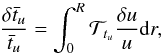 (17)where
 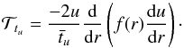 (18)The weight function f(r) must be chosen according to a number of criteria: it has to be sensitive to the core regions where the profile changes; it has to have a low amplitude at the boundaries of the domain, allowing us to do the integration by parts necessary for obtaining δu in the expression; and it should be possible to fit the target function associated with this f(r) using structural kernels from a restricted number of frequencies. Moreover, Eq. (18) being related to linear perturbations, it is clear that non-linear effects should not dominate the changes of this indicator3. We also know that the amplitude of the structural kernels is 0 in the centre, so f(r) should also satisfy this condition.
We define the weight function as: 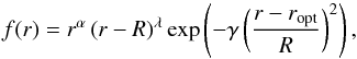 (19)which means that we have four parameters to adjust. The case of ropt is quickly treated. Since we know that the changes will be localised in the lobes developing in the core regions, we chose to put ropt = 0, and α and λ should be at least 1, so that the integration by part is exact and the central limit for the target function and the structural kernels is the same. Gamma depends on the effects of the non-linearities. However, since we have to perform a second derivative of u a more practical concern appears: we do not want to be influenced by the effects of the discontinuity at the boundary of the convective envelope. Ultimately, we use the following set of parameters: α = 1, λ = 2, γ = 7, and ropt = 0. One could argue that the optimal choice for ropt would be either at the maximum of the second lobe or between both lobes to obtain the maximal sensitivity in the structural variations. These values were also tested, but the results were a little less accurate than using ropt = 0 and they involved higher inversion coefficients and, hence, higher error magnification. We illustrate the weighted profile obtained for this optimal set of parameters in the right-hand side panel of Fig. 5. Furthermore, Eq. (17) is satisfied up to 5%, so we can try to carry out inversions for this indicator. It is also important to note that for the sake of simplicity, we do not choose to change the values of these parameters with the model, which would only bring additional complexity to the problem.
Because of the target function  , we can now carry out inversions for the integrated quantity tu using the linear SOLA inversion technique (Pijpers & Thompson 1994). But first, we should recall the purpose of inversions and our adaptation of the SOLA technique to integrated quantities. Historically, inversions have been used to obtain seismically constrained structural profiles (Basu et al. 1996b) as well as rotational profiles (Schou et al. 1994) in helioseismology. However, none of these methods are suited for the inversions we wish to carry here. As discussed in Buldgen et al. (2015), the SOLA inversion technique, which uses a so-called kernel-matching approach is well suited to our purpose. Indeed, this approach allows us to define custom-made target functions that will be used to build a cost function, here denoted
  . In the case of the tu quantity, one has the definition
 ![Mathematical equation: \begin{eqnarray} \mathcal{J}_{t_{u}}& = &\int_{0}^{1}\left[K_{\mathrm{Avg}}-\mathcal{T}_{t_{u}}\right]^{2}{\rm d}x +\beta \int_{0}^{1}K^ {2}_{\mathrm{Cross}}{\rm d}x + \tan(\theta) \sum^{N}_{i}(c_{i}\sigma_{i})^{2} \nonumber \\ &&+ \eta \left[\sum^{N}_{i}c_{i}-k \right], \end{eqnarray}](/articles/aa/full_html/2015/11/aa26390-15/aa26390-15-eq123.png) (20)where KAvg is the so-called averaging kernel and KCross is the so-called cross-term kernel defined as follows for the (u,Γ1) structural pair (for (u,Y), replace by
(20)where KAvg is the so-called averaging kernel and KCross is the so-called cross-term kernel defined as follows for the (u,Γ1) structural pair (for (u,Y), replace by  and
and  by
by  ):
):
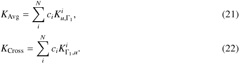 The symbols θ and β are free parameters of the inversion. Here, θ is related to the compromise between the amplification of the observational error bars (σi) and the fit of the kernels, whereas β is allowed to vary to give more weight to the elimination of the cross-term kernel. In this expression, N is the number of observed frequencies, the ci are the inversion coefficients, used to determine the correction that will be applied on the tu value. Eta is a Lagrange multiplier and the last term appearing in the expression of the cost-function is a supplementary constraint applied to the inversion that is presented in Sect. 3.2.
If the observed target and the reference model have the same radius, the inversion will measure the value of tu for the observed target. However, if this condition is not met, the inversion will produce a scaled value of this indicator. By defining integral equations such as Eq. (15), or even Eq. (1), we have seen in Sect. 2.1 that we made the hypothesis that both the target and the reference model had the same radius. However, because the frequencies scale with  , the inversion will preserve the mean density of the observed target. Therefore, we are implicitly carrying out the inversion for a scaled target homologous to the observed target, which has the radius of the reference model but the mean density of the observed target. Simple reasoning demonstrates that the mass of this scaled target is:
  . Thus, because tu scales as M2, there is a difference between the target value
  and the measured value,
  . Consequently, we can write the following equations:
 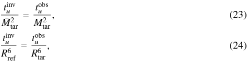 where we have used the definition of
  to express the mass dependencies as radius dependencies. Therefore, we use Eq. (24) as a criterion to determine whether the inversion was successful or not.
3.2. Non-linear generalisation
This section presents a general approach to the non-linear generalisation presented in Reese et al. (2012) and Buldgen et al. (2015) for any type of global characteristic that can scale with the mass of the star. It is obvious that we can say that the frequencies scale as M1/2. Of course, they scale as the mean density, namely  . However, since the inversion works with a fixed radius and implicitly scales the target to the same radius as the reference model, the iterative process associated with this non-linear generalisation will never change the model radius. Therefore, we do not take this dependence into account and simply work on the mass dependence. We let A be a global characteristic, related to the mass of the star. It is always possible to define a factor k so that:
  (25)And we directly obtain:
  (26)However, using the definition of the inverted correction of A, one has:
  (27)where ci are the inversion coefficients. Using the same reasoning as in Buldgen et al. (2015) and Reese et al. (2012), we define the inversion as “unbiased” (a term that should not be taken in the statistical sense.) if it satisfies the condition
  (28)Now we can define an iterative process using the scale factor
  . We scale the reference model (in other words, multiply its mass and density by s2, its pressure by s4, leaving Γ1 unchanged), carry out a second inversion, then define a new scale factor and so on until no further correction is made by the inversion process. In other words, we search for the fixed point of the equation of the scale factor. At the jth iteration, we obtain the following equation for the inversion value of A:
 ![Mathematical equation: \begin{eqnarray} A_{\mathrm{inv}}=A_{\mathrm{ref}}s^{k-1}_{j}\left[s_{j}+\sum_{i}c_{i}\frac{\delta \nu_{i}}{\nu_{i}} +k(1-s_{j}) \right]. \end{eqnarray}](/articles/aa/full_html/2015/11/aa26390-15/aa26390-15-eq154.png) (29)This can be written in terms of the scale factor alone, noting that at the jth iteration,
(29)This can be written in terms of the scale factor alone, noting that at the jth iteration,  :
: ![Mathematical equation: \begin{eqnarray} s^{k}_{j+1}=s_{j}^{k-1}\left[s_{j}+\sum_{i}c_{i}\frac{\delta \nu_{i}}{\nu_{i}} +k(1-s_{j}) \right]. \end{eqnarray}](/articles/aa/full_html/2015/11/aa26390-15/aa26390-15-eq156.png) (30)The fixed point is then obtained,
(30)The fixed point is then obtained,  (31)and can be used directly to obtain the optimal value of the indicator A. We can also carry out a general analysis of the error bars treating the observed frequencies and Ainv as stochastic variables:
  with ϵi and ϵA being the stochastic contributions to the variables. Using the hypothesis that ϵi ≪ 1 we obtain the following equation for the error bars:
 ![Mathematical equation: \begin{eqnarray} \sigma_{A}=A_{\rm ref}\left[\frac{1}{k} \sum_{i}c_{i}\frac{\nu_{i}^{\mathrm{obs}}}{\nu^{\mathrm{ref}}_{i}} \right]^{k-1}\sqrt{\left(\sum_{i}c_{i}\sigma_{i}\right)^{2}}. \end{eqnarray}](/articles/aa/full_html/2015/11/aa26390-15/aa26390-15-eq163.png) (34)We note that in the particular case of the indicator tu, k = 4. Indeed, tu ∝ M2 whereas ν ∝ M1/2.
(34)We note that in the particular case of the indicator tu, k = 4. Indeed, tu ∝ M2 whereas ν ∝ M1/2.
Characteristics of the 6 targets.
Inversion results for the 6 targets using the (u,Γ1) kernels.
3.3. Tests using various physical effects
To test the accuracy of the SOLA technique applied to the tu indicator, we carried out the same test as in Buldgen et al. (2015) using stellar models that would play the role of observed targets. These models included physical phenomena not taken into account in the reference models. A total of 13 targets were constructed, with masses of 0.9 M⊙, 1.0 M⊙ and 1.1 M⊙ but to avoid redundancy, we only present six that are representative of the mass and age ranges and of the physical effects considered in our study. We tested various effects for each mass. These effects fell into the following categories: those that come from microscopic diffusion using the approach presented in Thoul et al. (1994) (multiplying the atomic diffusion coefficients by a factor given in the last line of Table 14), those caused by a helium abundance mismatch, those that result from a metallicity mismatch, and those that stem from using a different solar heavy-element mixture. For the last case, the target was built using the Grevesse & Noels (1993) (GN93) abundances and the reference model was built using the Asplund et al. (2009) (AGSS09) abundances.
All targets and reference models were built using version 18.15 of the Code Liégeois d’Evolution Stellaire (CLES) stellar evolution code (Scuflaire et al. 2008b) and their oscillations frequencies were calculated using the Liège oscillation code (LOSC, Scuflaire et al. 2008a). Table 1 summarises the properties of the six targets presented in this paper. The selection of the reference model was based on the fit of the large and small separation for 60 modes with n = 7−26 and ℓ = 0−2 using a Levenberg-Marquardt minimisation code. The use of supplementary constraints will be discussed in Sect. 5 whereas the effects of the selection of the modes will be discussed in Sect. 4. The choice of 60 frequencies is motivated by the number of observed frequencies for the system 16Cyg A - 16Cyg B by Kepler, which is between 50 and 60 (Verma et al. 2014). The inversions were carried out using the (u,Y) and the (u,Γ1) structural kernels.
Inversion results for the 6 targets using the (u,Y) kernels.
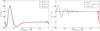 |
Fig. 6 Left: averaging kernels for both structural pairs and their respective targets. The red and blue curves are nearly identical, so that only the red curve is visible. Right: cross-term kernels for both structural pairs, the target being 0. |
If the inversion of tu shows that there are differences between the target and the reference model, then we know that the core regions are not properly represented. Whether these differences arise from atomic diffusion or a helium abundance mismatch, the tu indicator alone could not answer this question5. Therefore, the philosophy we adopt in this paper is the following: Is the inversion able to correct mistakes in the reference models? If so, within what range of accuracy? The capacity of disentangling different effects is partially illustrated in Sect. 5, but additional indicators are still required to provide the best diagnostic possible given a set of frequencies.
The results are given in Table 2 for the (u,Γ1) kernels and Table 3 for the (u,Y) kernels along with the respective error contributions given according to the developments of Reese et al. (2012) and Buldgen et al. (2015). We denote these error contributions: εAvg, εCross, εRes. These errors contributions are defined as
![Mathematical equation: \begin{eqnarray} && \varepsilon_{\mathrm{Avg}}=\int_{0}^{1}\left[K_{\mathrm{Avg}}-\mathcal{T}_{t_{u}} \right]\frac{\delta u}{u}{\rm d}x, \\ && \varepsilon_{\mathrm{Cross}}=\int_{0}^{1} K_{\mathrm{Cross}}\frac{\delta \Gamma_{1}}{\Gamma_{1}}{\rm d}x, \end{eqnarray}](/articles/aa/full_html/2015/11/aa26390-15/aa26390-15-eq301.png) if the (u,Γ1) couple is used. If one prefers the (u,Y), εCross becomes
if the (u,Γ1) couple is used. If one prefers the (u,Y), εCross becomes  (37)Finally, εRes is associated with the residual contribution, in the sense that it is what remains after one has taken into account both εCross and εAvg. The target function and their fits are illustrated in Fig. 6 for Target4. As we can see from Tables 2 and 3, we obtain accurate results for all cases. This means that the inversion is successful and that the regularisation process is sufficient for the values β = 10-6 and θ = 10-5.
We see in the fifth column of Tables 2 and 3 that the averaging kernel fit is usually the dominant error contribution. In the next sections, we see how this result changes with the modes used or with the quality of the reference model. If we analyse the cross-term error contribution, we see that it is generally much less important than the averaging kernel mismatch error. We also see that despite the high amplitude of the cross-term kernels associated with Γ1 shown in Fig. 6, the real error is quite small and often smaller than the error associated with the helium cross-term kernel. This is due not only to the small variations in Γ1 between target and reference model but also to the oscillatory behaviour of the Γ1 cross-term kernel. In contrast, the cross-term kernel of the (u,Y) kernel has a smaller amplitude, but nearly no oscillatory behaviour and is larger in the surface regions, where the inversion is naturally less robust. Nonetheless, the results of the (u,Y) kernels also show some compensation. We also note that they tend to have larger residual errors. However, there is no clear difference in accuracy between the (u,Γ1) and the (u,Y) kernels. In the case of Target2, we see that although the results are slightly improved, the reference value is within the error bars of the inversion results. In an observed case, this would mean that the reference model is already very close to the target as far as the indicator tu is concerned. However, we wish to point out that it seems rather improbable that the only difference between a static model and a real observed star would be in its heavy-element mixture.
Analysing the residual contribution is slightly more difficult, since it includes each and every supplementary effect: surface terms, non-linear contributions, errors in the equation of state (when using kernels related to Y), etc. In this study, we can see that the residual error is well constricted. This is not the case, for example, if the parameter θ is chosen to be very small, or if the scaling effect is not taken into account6. In fact, the θ parameter is a regularizing parameter, in the sense that it does not allow the inversion coefficients to take on extremely high values. In that case, the inversion would be completely unstable because a slight error in the fit would be amplified and would lead to incorrect results. This is quickly understood knowing that the inversion coefficients are used to recombine the frequencies as  (38)with N the total number of observed frequencies. Where this equation is subject to the uncertainties in Eqs. (17) and (5) (or, respectively Eq. (13)), any error will be dramatically amplified by the inversion process. Therefore there is no gain in reducing θ since at some point, the uncertainties behind the basic equation of the inversion process will dominate and lead the method to failure. In this case, the inversion problem is not sufficiently regularised. Such an example is presented and analysed in the next section.
4. Impact of the type and number of modes on the inversion results
When carrying out inversions on observed data, we are limited to the observed modes. Therefore the question of how the inversion results depend on the type of modes is of utmost importance. The reason behind this dependence is that different frequencies are associated with different eigenfunctions, in other words different structural kernels, sensitive to different regions of the star. Therefore, the inverse problem will vary for each set of modes because the physical information contained in the observational data changes. Hence, we studied four targets using seven sets of modes. As in Sect. 3.3, we wish to avoid redundancy and so present our results for one target, namely Target3, and five different frequency sets. As a supplementary test case, we defined two target models with the properties of 16CygA and 16CygB found in the litterature (Metcalfe et al. 2012; White et al. 2013; Verma et al. 2014). Using these properties, we added strong atomic diffusion to the 16CygA model and used Z = 0.023 as well as the GN93 mixture for 16CygB. In constrast, the reference models used Z = 0.0122 and the AGSS09 mixture. The characteristics of these models are also summarised in Table 4, where we used the set of observed modes given by Verma et al. (2014) and ignored the isolated ℓ = 3 modes for which there was no possibility to define a large separation.
All the sets for the test cases of this section are summarised in Table 5. The reference model was chosen as in Sect. 3.3, using the arithmetic average of the large and small frequency separations as constraints for its mass and age. With these test cases, we first analyse whether the inversion results depend on the values of the radial order n of the modes, with the help of the frequency Sets 1, 2 and 3 (see Table 5). Then we analyse the importance of the ℓ = 3 modes for the inversion using Sets 4 and 5.
The inversion results for all these targets and sets of mode are presented in Tables 6 and 7 for the (u,Γ1) kernels. A first conclusion can be drawn from the results using Sets 1, 2 and 3: low n are important for ensuring an accurate results. In fact, Set 2 provides much better results than Set 1,. Even using Set 3 (which is only Set 1 extended up to n = 34 for each ℓ) does not improve the results any further. This means that modes with n> 27 are barely used to fit the target.
This first result can be interpreted in a variety of ways. Firstly, using mathematical reasoning, we can say that the kernels associated with higher n have high amplitudes in the surface regions and are therefore not well suited to probing central regions. Another way to interpret this problem follows: When we use modes with high n, we come closer to the asymptotic regime, and the eigenfunctions are described by the JWKB approximation, all of which have a similar form and do not therefore provide useful additional information. Based on this, we see a clear difference between inverted structural quantities and the information deduced from asymptotic relations, which requires high n values to be valid, thereby highlighting the usefulness of inversions.
Characteristics of 16CygA and 16CygB clones.
The question of the importance of the modes ℓ = 3 is also quickly answered from the results obtained with Set 4 and 5. For these test cases, we reach very good accuracy even without n ≤ 9 unlike the previous test case using Set 2. Moreover, we use even fewer frequencies than for the first three sets. In fact, this is crucial to determine whether one can apply an inversion in an observed case, since a few ℓ = 3 modes can change the results and make the inversion successful.
To further illustrate the importance of the octupole modes, we use the 16CygA and 16CygB clones to carry out inversions for their respective observed frequency sets. In a first test case, we use all frequencies and reach a reasonable accuracy for both targets. In the second test case, we do not use the octupole modes and we can observe a drastic change in accuracy. These results are illustrated in Table 7, where the notation "Small" (for small frequency set) has been added to the lines associated with the results obtained without using the ℓ = 3 modes.
Looking again at the results for 16CygA, we see that although the inversion improves the value of tu, the reference value lies within the observational error bars of the inverted result. The case of the truncated set of frequencies is even worse, since the inverted result is less accurate than the reference value. We therefore analysed the problem for the full frequency set. To do so we carried out a variety of inversions using higher values of θ. The results for θ = 10-4 are illustrated in Table 7. In this case we have lower error bars, but what is reassuring is that the result did not change drastically when we changed θ. This means that the problem is properly regularised around θ = 10-5 and θ = 10-4 and that we can trust the inversion results. Our advice is therefore to always look at the behaviour of the solution with the inversion parameters to see if there is any sign of compensation or other undesirable behaviour. In fact there is no law to select the value of θ and applying fixed values blindly for all asteroseismic observations is probably the best way to obtain unreliable results.
The case of the small frequency set is even more intriguing since the result improves greatly with θ = 10-4. The question that arises is whether the problem is not properly regularised with θ = 10-5 or whether we are faced with some fortuitous compensation effect that leads to very accurate results. If we are faced with fortuitous compensation, taking θ slightly larger than 10-4 or increasing β will drastically reduce the accuracy since any change in the linear combination will affect the compensation. However, if we are faced with a regularisation problem, the accuracy should decrease regularly with the change of parameters (since we are slightly reducing the quality of the fit with those changes). We emphasise again that one should not choose values of the inversion parameters where any small augmentation of the regularisation would drastically change the result. In this particular case, we were confronted with insufficient regularisation and choosing θ = 10-4 corrected the problem.
Sets of modes used to analyse the impact of the number and type of frequencies on the inversion results.
Inversion results for the 16CygA and 16CygB clones using the (u,Γ1) kernels.
Characteristics of Target7, Target8, and of the models obtained with the Levenberg-Marquardt algorithm.
5. Impact of the quality of the forward modelling process on the inversion results
In this section we present various inversion results using different criteria to select the reference model for the inversion. The previous results, only using the average large and small frequency separations as constraints for the mass and age of the model, are indeed a crude representation of the real capabilities of seismic modelling. It is well known that other individual frequency combinations can be used to obtain independent information on the core mixing processes and that we should adjust more than two parameters to describe the physical processes in stellar interiors.
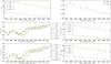 |
Fig. 7 Results of the fit using the Levenberg-Marquardt algorithm for the first target as a function of the observed frequency: the upper panel is associated with Model7.1 which used the average large frequency separation and the individual r01 and |


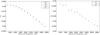 |
Fig. 8 Results of the fit using the Levenberg-Marquardt algorithm for the second target as a function of the observed frequency (colour online): the red dots are associated with Model8.1 which used individual r02 as constraints and the purple dots are associated with Model8.2 which used individual r02 and r01 as constraints. |
To carry out these test cases, we built two target models including microscopic diffusion. As before, we did not include this process in the reference models obtained by fitting the so-called 56 observed frequencies. We used the modes l = 0,n = 12−25; l = 1,n = 11−25; l = 2,n = 11−26; l = 3,n = 14−24. The characteristics of the targets are summarised in Table 8 along with those of the best models obtained through seismic modelling. Table 9 contains information on the various constraints and free parameters used for the fit. We used various seismic constraints such as the individual large and small frequency separations, the individual r01 and r02, defined as  The free parameters were chosen to match what is done when trying to fit observations, although the final quality of the fit is much higher than one expects from an observed case, as illutrasted in Fig. 7 for Target77 and Fig. 8 for Target8.
Constraints and free parameters used for the Levenberg-Marquardt fit.
Here one should note that the arithmetic average of the large frequency separations were fitted to within 1% in addition to the individual quantities plotted in Fig. 8. In all these cases the inversion improved the value of tu. In some cases, the acoustic radius was not well fitted by the forward modelling process but the inversion could improve its determination. Table 11 illustrates the results of combined inversions, whereas Table 10 gives the results for all test cases. In fact, one could argue that the error contributions are not that different from what was obtained using only the average large and small frequency separations as constraints. However, our previous analysis of the dependence on the degree and radial order of the modes has shown us that having low n and l = 3 modes was the best way to ensure accuracy.
Inversion results for various fits with the Levenberg-Marquardt algorithm.
Combined (τ,tu) inversion results for various fits with the Levenberg-Marquardt algorithm.
Based on the above, the frequency set used for these test cases is of lower quality and this has been compensated for by the forward modelling process. To further illustrate the importance of the model selection, in Table 10 we repeat the results obtained by simply ajusting ⟨ Δν ⟩ and  that we denote as Model7.0. For Target7 we see that the dominant source of error contribution, εAvg is ± 6 to 10 times smaller than what is for Model7.0. As a result it is clear that using the information given by individual frequencies is crucial to ensure accurate results in observed cases.
The necessity of an acoustic radius inversion results from two aspects in the selection of the reference models. The first one is present in Model7.2; the change of α induced during the fit had an important impact on the upper regions and therefore a change in the acoustic radius was observable. The second one is present in Model8.1 and Model8.2, where the observational constraints were sensitive to core regions, except for the arithmetic average of the large frequency separations. In this case, the upper regions are less constrained and the inversion is still necessary. However, we note that in most cases the acoustic radius of the reference model was very accurate. This is due to the lack of surface effects in the target models. If we were to include non-adiabatic computations or differences in the convection treatment, differences would be seen in the acoustic radii of the targets and reference models, but it is clear from these test cases that the acoustic radius combined with tu alone is not sufficient to distinguish between effects of differences in helium abundance and effects of microscopic diffusion. We also note that when using the individual r02 along with the ⟨ Δν ⟩ (the test case of Model8.1), we obtain a very good fit of tu with the reference model. This is a consequence of the fact that r02 is very sensitive to core regions, and so the core characteristics are reproduced well. However, with the acoustic radius inversion, we note that the surface regions are not well fitted, and if we include r01, as done in the test case of Model8.2, we obtain a better fit of the acoustic radius, but tu is then less accurate. The inversion of the indicator tu informs us that the core regions are not reproduced well in this reference model. We can see that Model8.1 or Model7.2 and Model7.3 reproduce the indicator tu better. However, in all these cases the acoustic radius was not properly reproduced. Therefore the combined inversions indicate that something is wrong with the set of free parameters used because we cannot fit properly surface and core regions simultaneously, although the fit of the seismic constraints with the Levenberg-Marquardt algorithm is excellent in all cases.
We also mention that in all test cases carried out here, we did not consider the first age indicator t from Buldgen et al. (2015). In fact, the indicator t could also provide accurate results for Target7. However, its inaccuracy for older models has been observed during this entire study, and we recommend limiting its use to young stars8, where it can provide valuable information providing that the kernels are well optimised.
6. Conclusion
In this article, we have presented a new approach to constraining mixing processes in stellar cores using the SOLA inversion technique. We used the framework presented in Buldgen et al. (2015) to develop an integrated quantity, denoted tu, that is sensitive to the effects of stellar evolution and to the impact of additional mixing processes or mismatches in the chemical composition of the core. We based our choice solely on structural effects and considerations about the variational principle and the ability of the kernels to fit their targets.
The derivation of this new quantity was made possible using the approach of Masters (1979) to derive new structural kernels in the context of asteroseismology by solving an ordinary differential equation. We discussed the problem of the intrinsic scaling effect presented in Basu (2003) and discussed how it could affect the indicator tu. We tested its sensitivity to various physical changes between the target and the reference model and demonstrated that SOLA inversions are able to significantly improve the accuracy with which tu is determined, thereby indicating whether there is a problem in the core regions of the reference model.
We then analysed the importance of the number and type of modes in the observational data and concluded that the accuracy of an inversion of the indicator tu increased with multiple values of the degree, ℓ, and low values of the radial order, n. Following from this, we emphasise that the observation of ℓ = 3 modes is important for the inversion of the indicator tu since it can improve the accuracy without the need of low n modes. Such modes are difficult to observe. Indeed, only a few octupole modes have been detected for around 15% of solar-like stars with Kepler. The use of other observational facilities, such as the SONG network (Grundahl et al. 2007), might help us obtain richer oscillation spectra as far as octupole modes are concerned. The test cases for the 16CygA and 16CygB clones demonstrated that our method was applicable to current observational data and one could still carry out an inversion of tu without these modes. However, it is clear that this method will only be applicable to the best observational cases with Kepler, Plato or SONG.
We also analysed the impact of the selection of the reference model on the inversion results and concluded that using individual frequency combinations is far more efficient in terms of accuracy and stability for the inversion results. However, we noticed in supplementary tests that there was what could be called a resolution limit for the tu inversion which depends on the magnitude of the differences in the physics between the reference model and its targets but also on the weight given to the core in the selection of the reference model. (See for example the case of Model8.1 and the associated discussion.) This leads to the conclusion that supplementary independent integrated quantities should be derived to help us distinguish between various physical effects and improve our sensitivity to the physics of stellar interiors. Nevertheless, the test cases of Sect. 5 showed that the SOLA method is much more sensitive than the forward modelling process used to select the reference model (here a Levenberg-Marquardt algorithm) and could indicate whether the set of free parameters used to describe the model is adequate.
The method of adjoint equations previously described could also be used but would require an additional hypothesis to replace the missing boundary condition.
However, these can be neglected when compared to other uncertainties on the structural properties of observed stars.
Otherwise, using the SOLA technique, which is linear, would be impossible.
These values might seem excessive regarding the reliability of the implementation of diffusion. We stress here that our goal was to witness the impact of significant changes on the results. However, other processes or mismatches could alter the gradient and thus be detected by the inversion.
To completely constrain the changes that are a consequence of multiple additional mixing processes with only one structural indicator is of course impossible.
In which case one would be searching for a result that is impossible to obtain.
We did not present the fit of the individual large frequency separations for Model7.1 to avoid redundancy with Model7.2 and Model7.3.
We chose not to present these results and to focus our study on the tu indicator.
Acknowledgments
G.B. is supported by the FNRS (“Fonds National de la Recherche Scientifique”) through a FRIA (“Fonds pour la Formation à la Recherche dans l’Industrie et l’Agriculture”) doctoral fellowship. D.R.R. is currently funded by the European Community’s Seventh Framework Programme (FP7/2007-2013) under grant agreement no. 312844 (SPACEINN), which is gratefully acknowledged. This article made use of an adapted version of InversionKit, a software developed in the context of the HELAS and SPACEINN networks, funded by the European Commissions’s Sixth and Seventh Framework Programmes.
References
- Asplund, M., Grevesse, N., Sauval, A. J., & Scott, P. 2009, ARA&A, 47, 481 [NASA ADS] [CrossRef] [Google Scholar]
- Basu, S. 2003, Ap&SS, 284, 153 [NASA ADS] [CrossRef] [Google Scholar]
- Basu, S., Christensen-Dalsgaard, J., Perez Hernandez, F., & Thompson, M. J. 1996a, MNRAS, 280, 651 [NASA ADS] [Google Scholar]
- Basu, S., Christensen-Dalsgaard, J., Schou, J., Thompson, M. J., & Tomczyk, S. 1996b, BASI, 24, 147 [Google Scholar]
- Brown, T. M., Christensen-Dalsgaard, J., Weibel-Mihalas, B., & Gilliland, R. L. 1994, ApJ, 427, 1013 [NASA ADS] [CrossRef] [Google Scholar]
- Buldgen, G., Reese, D. R., Dupret, M. A., & Samadi, R. 2015, A&A, 574, A42 [NASA ADS] [CrossRef] [EDP Sciences] [Google Scholar]
- Däppen, W., Gough, D. O., Kosovichev, A. G., & Thompson, M. J. 1991, in Lecture Notes in Physics, Challenges to Theories of the Structure of Moderate-Mass Stars, eds. D. Gough, & J. Toomre (Berlin: Springer Verlag), 388, 111 [Google Scholar]
- Deheuvels, S., Doğan, G., Goupil, M. J., et al. 2014, A&A, 564, A27 [NASA ADS] [CrossRef] [EDP Sciences] [Google Scholar]
- Dupret, M.-A. 2008, Commun. Asteroseismol., 157, 16 [NASA ADS] [Google Scholar]
- Dziembowski, W. A., Pamyatnykh, A. A., & Sienkiewicz, R. 1990, MNRAS, 244, 542 [NASA ADS] [Google Scholar]
- Eggenberger, P., Meynet, G., Maeder, A., et al. 2010, A&A, 519, A116 [NASA ADS] [CrossRef] [EDP Sciences] [Google Scholar]
- Elliott, J. R. 1996, MNRAS, 280, 1244 [NASA ADS] [CrossRef] [Google Scholar]
- Elsworth, Y., Howe, R., Isaak, G. R., McLeod, C. P., & New, R. 1990, Nature, 347, 536 [NASA ADS] [CrossRef] [Google Scholar]
- Gough, D. O., & Thompson, M. J. 1991, The inversion problem, eds. A. N. Cox, W. C. Livingston, & M. S. Matthews (Tucson: The University of Arizona Press), 519 [Google Scholar]
- Grevesse, N., & Noels, A. 1993, Physica Scripta Volume T, 47, 133 [Google Scholar]
- Grundahl, F., Kjeldsen, H., Christensen-Dalsgaard, J., Arentoft, T., & Frandsen, S. 2007, Commun. Asteroseismol., 150, 300 [NASA ADS] [CrossRef] [Google Scholar]
- Kosovichev, A. G. 1999, J. Comput. Appl. Math., 109, 1 [NASA ADS] [CrossRef] [Google Scholar]
- Lebreton, Y., Goupil, M. J., & Montalbán, J. 2014a, in EAS Publ. Ser., 65, 99 [Google Scholar]
- Lebreton, Y., Goupil, M. J., & Montalbán, J. 2014b, in EAS Publ. Ser., 65, 177 [Google Scholar]
- Masters, G. 1979, Geophys. J. Int., 57, 507 [NASA ADS] [CrossRef] [Google Scholar]
- Metcalfe, T. S., Chaplin, W. J., Appourchaux, T., et al. 2012, ApJ, 748, L10 [NASA ADS] [CrossRef] [Google Scholar]
- Miglio, A., Girardi, L., Rodrigues, T. S., Stello, D., & Chaplin, W. J. 2015, Astrophys. Space Sci. Proc., 39, 11 [Google Scholar]
- Pijpers, F. P., & Thompson, M. J. 1994, A&A, 281, 231 [NASA ADS] [Google Scholar]
- Rauer, H., Catala, C., Aerts, C., et al. 2014, Exper. Astron., 38, 249 [Google Scholar]
- Reese, D. R. 2013, A&A, 555, A148 [NASA ADS] [CrossRef] [EDP Sciences] [Google Scholar]
- Reese, D. R., Marques, J. P., Goupil, M. J., Thompson, M. J., & Deheuvels, S. 2012, A&A, 539, A63 [NASA ADS] [CrossRef] [EDP Sciences] [Google Scholar]
- Roxburgh, I. W. 2010, Ap&SS, 328, 3 [NASA ADS] [CrossRef] [Google Scholar]
- Roxburgh, I. W. 2015, A&A, 574, A45 [NASA ADS] [CrossRef] [EDP Sciences] [Google Scholar]
- Schou, J., Christensen-Dalsgaard, J., & Thompson, M. J. 1994, ApJ, 433, 389 [NASA ADS] [CrossRef] [Google Scholar]
- Scuflaire, R., Montalbán, J., Théado, S., et al. 2008a, Ap&SS, 316, 149 [NASA ADS] [CrossRef] [Google Scholar]
- Scuflaire, R., Théado, S., Montalbán, J., et al. 2008b, Ap&SS, 316, 83 [NASA ADS] [CrossRef] [Google Scholar]
- Tassoul, M. 1980, ApJS, 43, 469 [NASA ADS] [CrossRef] [Google Scholar]
- Thoul, A. A., Bahcall, J. N., & Loeb, A. 1994, ApJ, 421, 828 [NASA ADS] [CrossRef] [Google Scholar]
- Verma, K., Faria, J. P., Antia, H. M., et al. 2014, ApJ, 790, 138 [NASA ADS] [CrossRef] [Google Scholar]
- White, T. R., Huber, D., Maestro, V., et al. 2013, MNRAS, 433, 1262 [NASA ADS] [CrossRef] [Google Scholar]
All Tables
Sets of modes used to analyse the impact of the number and type of frequencies on the inversion results.
Characteristics of Target7, Target8, and of the models obtained with the Levenberg-Marquardt algorithm.
Combined (τ,tu) inversion results for various fits with the Levenberg-Marquardt algorithm.
All Figures
|
Fig. 1 Verification of Eq. (1) for a set of 120 modes with the · being the 40 radial modes, the × being the 40 dipolar modes and the + being the 40 quadrupolar modes. The left plot illustrates this verification for the (ρ,c2) couple when no scaling is applied to c2 whereas the right plot illustrates the same verification for the (ρ,c2) couple when scaling is applied to c2, as well as the (ρ,Γ1) couple where no scaling is needed. |
| In the text | |
|
Fig. 2 Left: plot illustrating the verification of Eq. (10) for n = 15, ℓ = 0 kernel K15,0, where ℐu,Γ1 is the right-hand side of this equation and ℛ is the residual. Right: same test as in Fig. 1 for the (u,Γ1) kernels. |
| In the text | |
 |
Fig. 3 Same as Fig. 2 for the (u,Y) kernels. |
| In the text | |
|
Fig. 4 Structural kernels for the n = 15, ℓ = 0 mode associated with the (u,Γ1) couple on the left hand side and with the (u,Y) couple on the right hand side. |
| In the text | |
|
Fig. 5 Left panel: structural changes in the scaled |
| In the text | |
|
Fig. 6 Left: averaging kernels for both structural pairs and their respective targets. The red and blue curves are nearly identical, so that only the red curve is visible. Right: cross-term kernels for both structural pairs, the target being 0. |
| In the text | |
|
Fig. 7 Results of the fit using the Levenberg-Marquardt algorithm for the first target as a function of the observed frequency: the upper panel is associated with Model7.1 which used the average large frequency separation and the individual r01 and |
| In the text | |
|
Fig. 8 Results of the fit using the Levenberg-Marquardt algorithm for the second target as a function of the observed frequency (colour online): the red dots are associated with Model8.1 which used individual r02 as constraints and the purple dots are associated with Model8.2 which used individual r02 and r01 as constraints. |
| In the text | |
Current usage metrics show cumulative count of Article Views (full-text article views including HTML views, PDF and ePub downloads, according to the available data) and Abstracts Views on Vision4Press platform.
Data correspond to usage on the plateform after 2015. The current usage metrics is available 48-96 hours after online publication and is updated daily on week days.
Initial download of the metrics may take a while.