© ESO, 2015

1. Introduction

Knowing the Milky Way’s chemical composition and its chemical abundance can lead us to understand how the Milky Way has formed and evolved. With time, the amount of heavy elements in a galaxy increases as new stars are born and die. Studies of elemental composition of stars will give information about the environment in which they were born. This, in turn, helps us to construct the evolution history of our Galaxy. For this reason, it is important to derive accurate abundances of stars.

Elemental abundances can be derived by comparing an observed stellar spectrum with a synthetic spectrum. This approach requires atomic data, meaning oscillator strengths (f-values) and wavelengths. The measured equivalent width of a line is directly proportional to the abundance of the element and the f-value. The lack of atomic data makes it difficult to compare the observed and synthetic stellar spectra. Thus, an accurate and complete set of oscillator strengths and wavelengths are crucial for abundance analysis.

In the periodic table, scandium is between the α-elements, e.g. O, Mg, Si, S, Ca, and the iron peak elements, such as V, Cr, Mn, Fe. The formation scenarios of α-elements and iron peak elements have been studied in detail. Stars that end their lives in supernova type II explosions are responsible for producing α-elements, whereas stars that die in supernova type Ia contribute to the formation of iron peak elements and yet there is no clear picture of how scandium is formed (Nissen et al. 2000; François et al. 2004; Zhang et al. 2008; Battistini & Bensby 2015).

Studies of F and G stars may provide insight into the creation of scandium. However, the abundance varies in these stars. There seems to be a disagreement in the scandium abundance pattern. In some studies, scandium is overabundant relative to iron (Zhao & Magain 1990; Nissen et al. 2000), whereas the others found no deviations (Gratton & Sneden 1991; Prochaska & McWilliam 2000). Furthermore, scandium is an important element for understanding Am and Fm stars, which are overabundant in iron peak elements but underabundant in Sc and Ca (Leblanc & Alecian 2008; Alecian et al. 2013). In addition to these, some studies cannot be completed owing to the quality of oscillator strengths in the infrared region (Schmidt et al. 2006). Improved atomic data with small uncertainties in oscillator strengths can help in solving these problems.

The scandium abundance in the Sun was determined by Grevesse et al. (1996) to be 3.18 ± 0.10 dex, and by Zhang et al. (2008) 3.13 ± 0.05 dex and by Asplund et al. (2009) to be 3.15 ± 0.04 dex. These values are consistent within the error bars. A high quality laboratory measurement of oscillator strengths with small uncertainties is a requirement for determining the accurate abundance of scandium in the solar photosphere.

In astrophysical applications, log(gf) values are usually used, where g is the statistical weight of the lower level and f is the oscillator strength (f-value). Parkinson et al. (1976) derived the experimental log(gf) values for Sc i lines involving the ground state in the optical region. Lawler & Dakin (1989) measured experimental log(gf) values for lines in the optical region involving the ground state or to the 4s ⁴F term. For other transitions, generally semi-empirical values of Kurucz (2009) are the favoured ones. In addition, Öztürk et al. (2014) calculated the oscillator strengths of neutral scandium with the Cowan code and the quantum defect orbital code (CDOT) methods but did not include any near-infrared transitions. To our knowledge, there are no experimental oscillator strengths of Sc i lines in the infrared region.

In recent years, infrared spectroscopy has become important for observing astronomical objects. Both new generation of ground-based telescopes and space telescopes, which work in the infrared region, demand complete and accurate atomic data. Atomic data of scandium are scarce in the infrared region and missing data constrain analysis of a stellar spectrum recorded with new-generation advanced instruments and, as a result, limit the construction of a galactic evolution model.

In this work, we measured accurate wavelengths and oscillator strengths of Sc i lines from high-resolution laboratory measurements in the infrared region from the upper odd parity 4p ⁴F^o, ⁴D^o, ²D^o, ²P^o, ⁴G^o, ²G^o and even parity 4s ²P, ²S terms. Section 2 describes the branching fraction measurements. In addition, this section includes the experimental setup we used during our measurements, calibration of wavenumbers, and the uncertainty calculations. In Sect. 3 we present our results with their uncertainties and a comparison of our results with previous studies.

2. Materials and methods

2.1. Branching fraction measurements

The oscillator strength, f-value, is related to the transition probability for electric dipole transitions by $\mathit{f}\mathrm{=}\frac{{\mathit{g}}_{\mathrm{u}}}{{\mathit{g}}_{\mathrm{l}}}{\mathit{\lambda }}^{\mathrm{2}}{\mathit{A}}_{\mathrm{ul}}\mathrm{1.499}\mathrm{\times }{\mathrm{10}}^{-16}\mathit{,}$(1)where g_u is the statistical weight of the upper level, g_l the statistical weight of the lower level, λ the wavelength of the transition in Å, and A_ul the transition probability in s^-1 between the upper level u and the lower level l.

The branching fraction (BF) for a given transition from the upper level u to the lower level l is defined as the ratio of the transition probability, A_ul, of the transition to the sum of all transitions from the same upper level to all lower states i. The transition probability is proportional to the transition line intensity; therefore, $\mathit{B}{\mathit{F}}_{\mathrm{ul}}\mathrm{=}\frac{{\mathit{A}}_{\mathrm{ul}}}{{\sum }_{\mathit{i}}{\mathit{A}}_{\mathrm{u}\mathit{i}}}\mathrm{=}\frac{{\mathit{I}}_{\mathrm{ul}}}{{\sum }_{\mathit{i}}{\mathit{I}}_{\mathrm{u}\mathit{i}}}\mathrm{·}$(2)Lifetime measurements are complementary to BF derivations. The radiative lifetime of the upper level, τ_u, is the inverse sum of all transition probabilities from the same upper level τ_u = 1/ ∑ _iA_ui. The transition probability of a line can be derived by combining experimental BFs and radiative lifetimes; ${\mathit{A}}_{\mathrm{ul}}\mathrm{=}\frac{\mathit{B}{\mathit{F}}_{\mathrm{ul}}}{{\mathit{\tau }}_{\mathrm{u}}}\mathrm{·}$(3)We derived transition probabilities, A_ul, with the help of Eq. (3) and converted these values to f-values using Eq. (1).

To derive accurate BFs, all transitions from the same upper level should be included. In this work, some upper energy levels had transitions in two different spectral regions recorded with different detectors. In such cases, because BFs require only the relative intensities, the spectra have to be put on a same relative intensity scale by using a normalisation factor. This normalisation factor was determined from the Sc i lines, which were visible in both spectra.

Figure 1 shows the partial energy level diagram of Sc i levels. In this figure we have marked the transitions that appeared in our spectra. Transition lines from the same upper level were predicted from the Kurucz (2009) database and from Ben Ahmed & Verges (1977). These lines were identified in our spectra by using FTS analysis software GFit (Engström 1998, 2014).

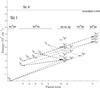Fig. 1 Partial energy level diagram of Sc i levels showing the observed transitions in the measurements.

Sc I has only one stable isotope, ⁴⁵Sc, with a nuclear spin I = 7/2, so Sc i lines show hyperfine splitting (hfs). Interaction between the nuclear spin and the total angular momentum splits energy levels into the hyperfine structure. This splitting appears as a resolved line splitting or a line broadening in a spectrum. Unsuccessful treatment of hfs leads to incorrect abundances, as much as several tenths of a dex (Nielsen et al. 2000). For lines with negligible hfs, one can fit a Voigt profile to the line and measure the central wavenumber and intensity. However, this is not the case for hfs. Having hfs gives rise to a difficulty in fitting a line profile since every fine-structure transition appears as a broadened or multi-component feature. For this reason, we defined the position of lines by the centre of gravity and instead of fitting a Voigt profile, we measured the integrated intensity under each measured line with the help of GFit. We applied this method for the cases in which we have a single line profile i.e. to test the accuracy. In all of these cases, fitting a line profile and taking an integrated intensity gave the same result.

2.2. Experimental setup

A water-cooled hollow cathode discharge lamp (HCL) was used as a source to produce scandium atoms. The HCL consists of a glass tube, anodes on each side, and an iron cathode in the middle. A small solid sample of scandium was placed in the iron cathode. The diameter of the inner cathode was 7 mm and the distance between anode and cathode was 20 mm. The light source was run with a pressure of 1.0 Torr (1.3 mbar), with different applied currents, ranges from 0.10 A to 0.60 A, and with argon or neon as a carrier gas. The best condition, i.e. the strongest lines, for the measurements was achieved with argon gas and with applied current of 0.60 A. The argon lines were used as reference lines for wavenumber calibration as described in Sect. 2.3.

The Sc i spectra were recorded using the high resolution Fourier transform spectrometer (FTS), Bruker IFS 125 HR, at the Lund Observatory (Edlén Laboratory). This instrument has the wavenumber range of 50 000–2000 cm^-1 (200–5000 nm) and the maximum resolving power of 10⁶ at 2000 cm^-1. The resolution of the FTS was set to 0.02 cm^-1 during measurements. We recorded the spectra with the indium antimonide (InSb) and silicon (Si) detectors, which are sensitive to different spectral regions.

The optical elements in FTS contribute to the response function of the instrument. Observed line intensities differ from the intrinsic line intensities, due to the wavelength dependent transmission of the spectrometer and optical elements. It was therefore required to find the response functions of two different detectors. After determining the response function, one can acquire the intrinsic line intensities by dividing the observed line intensities with the response function. A common way to determine the response function is to use an intensity calibrated reference. We used a tungsten filament lamp to calibrate the intensities of Sc i lines. This lamp in turn has been calibrated by the Swedish National Laboratory (SP) for spectral radiance in the range 40 000–4000 cm^-1 (250–2500 nm). If the radiance of the reference is known, one can determine the response function. Figure 2 shows the response function of the instrument with Si and with InSb detectors.

Fig. 2 Instrument response function with InSb (solid line) and Si (dashed line) detectors, respectively. Each curve is normalised to its highest point.

We recorded the spectrum of the tungsten lamp immediately before and after every scandium recording to verify the response of the instrument did not change during the measurements. For this reason the HCL and tungsten lamp were placed at the same distance from the FTS and a rotating mirror was used in order to change the light source (HCL or the Tungsten lamp) without moving the lamps. There were no changes in the spectra of the tungsten lamp taken before and after the HCL measurements, therefore one response function for each detector was used for calibration. Using intensity calibrated spectra, relative line intensities at the different regions were connected with a normalisation factor. This was done by using the Sc i lines in the overlapping region of the two detectors, see Fig. 2.

The spectra of Sc i lines were recorded with different currents. Higher current values help weaker lines to be visible, but introduce self-absorption. Self-absorption has a negative effect on line intensities e.g. it changes the observed line profile and gives an incorrect intensity. This in turn affects the BF measurements, see Eq. (2). The effect of self-absorption depends on the number density of atoms in the plasma and intensity of the line. The number density of the plasma increases by increasing the current applied to the HCL. The higher concentration of scandium ions in the plasma results in more lines affected by self-absorption. We performed a set of measurements with varying currents to determine if Sc i line intensities were affected by self-absorption at higher currents. Then we plotted normalised integrated intensity ratios of lines from the same upper level versus applied current. Integrated intensity ratios between lines from the same upper level must be same for different applied currents if there is no self-absorption. In our measurements some lines showed effects of self-absorption. In these cases, we extrapolated integrated intensity ratios to zero current, where self-absorption is assumed to be zero, and used these values to obtain correct relative intensities. Sikström et al. (2002) tested this method by comparing the self absorbed Fe I lines intensity ratios at zero current with the ratios derived by Blackwell et al. (1979) using absorption measurement. They found that the extrapolated intensity ratios agree with the Blackwell et al. (1979) intensity ratios. The correction of self-absorption introduce uncertainties in the BF determination.

2.3. Wavenumber calibration

The HeNe laser in the FTS determines the displacement of the FTS moving mirror and gives a multiplicative wavenumber scale to the spectrum. However, a non-parallel alignment with the incoming light beam adds a shift to the measured wavenumber. In addition to this difference, having a finite size aperture may lead to wavenumber shifts (Learner & Thorne 1988). The shift introduced by these effects is multiplicative. With a correction factor this shift can be calibrated; ${\mathit{\sigma }}_{\mathrm{true}}\mathrm{=}{\mathit{\sigma }}_{\mathrm{apparent}}\mathrm{(}\mathrm{1}\mathrm{+}{\mathit{k}}_{\mathrm{eff}}\mathrm{)}\mathit{.}$(4)In Eq. (4), σ_true denotes the corrected wavenumber, σ_apparent is the measured wavenumber, and k_eff is the correction factor. We used the wavenumbers of Ar i lines from Whaling et al. (2002), including the multiplicative correction by Sansonetti (2007), as a wavenumber standard for the wavenumber calibration of Sc i lines.

In principle, using only one calibration line is enough to fix the multiplicative constant, but several calibration lines can be employed for the purpose of increasing the wavenumber accuracy. We calculated a correction factor for each Ar i line and used the weighted mean of these factors.

We combined the errors in the determination of the multiplicative factor and the errors from centroiding the position of each line to estimate an absolute uncertainty of the observed wavenumbers of u(σ) = ± 0.001 cm^-1.

2.4. Uncertainties

The contribution to the f-value uncertainties comes from the uncertainty of the radiative lifetime and the uncertainty of the branching fractions. The branching fraction uncertainties contain the uncertainty of the intensity calibration lamp and the uncertainty that arises from using two different detectors, i.e. uncertainty of the normalisation factor and the contribution from the self-absorption correction.

The uncertainty of the line intensity (or the integrated intensity) and the uncertainty of the radiative lifetime are uncorrelated. Although BFs are dependent on each other, we treated them as independent in the uncertainty calculations. By including all the uncertainties from different effects described above, one can determine the total uncertainty of the BFs as specified in Sikström et al. (2002), $\begin{array}{cc}(\frac{\mathit{u}\mathrm{\left(}\mathit{BF}\mathrm{\right)}}{\mathit{BF}}{)}^{\mathrm{2}}\mathrm{=}\hspace{0.17em}& \mathrm{(}\mathrm{1}\mathrm{-}\mathrm{(}\mathit{BF}{\mathrm{)}}_{\mathit{k}}{\mathrm{)}}^{\mathrm{2}}(\frac{\mathit{u}\mathrm{\left(}{\mathit{I}}_{\mathit{k}}\mathrm{\right)}}{{\mathit{I}}_{\mathit{k}}})2\\ \mathrm{+}\sum _{\mathit{j}\hspace{0.17em}\ne \hspace{0.17em}\mathit{k}\mathrm{(}\mathrm{in}\hspace{0.17em}\mathit{P}\mathrm{)}}\mathrm{(}\mathit{BF}{\mathrm{)}}_{\mathit{j}}^{\mathrm{2}}((\frac{\mathit{u}\mathrm{\left(}{\mathit{I}}_{\mathit{j}}\mathrm{\right)}}{{\mathit{I}}_{\mathit{j}}}{)}^{\mathrm{2}}\mathrm{+}(\frac{\mathit{u}\mathrm{\left(}{\mathit{c}}_{\mathit{j}}\mathrm{\right)}}{{\mathit{c}}_{\mathit{j}}}{)}^{\mathrm{2}})& \end{array}$(5)In the first term on the right-hand side of Eq. (7), BF_k denotes the branching fraction of the line in question in the spectral region of the detector P and u(I_k) denotes the uncertainty in the measured intensity of the line k. The second term includes the BFs and measured intensity uncertainties of the other lines from the same upper level in the spectral region of detector P and the uncertainty of the calibration lamp u(c_j). The last term contains the BFs and measured intensity uncertainties of the lines in the spectral region of detector Q, the uncertainty of the calibration lamp, and the uncertainty of the normalisation factor, u(nf), between the spectral regions. The uncertainty of the calibration lamp, u(c_j), is 7% and the uncertainty of the normalisation factor is u(nf) = 5%. We used the uncertainties of the integrated intensity, u(I), from GFit and the relative uncertainty varies between 0.002% for the strong lines and 10% for the two weak lines and self-absorbed lines. The cases in which we had self absorbed lines, we included an uncertainty from self absorption correction as well. This uncertainty varies between 1% and 9%. From Eq. (3), the uncertainty of the f-values or the transition probability becomes $(\frac{\mathit{u}\mathrm{\left(}{\mathit{f}}_{\mathit{k}}\mathrm{\right)}}{{\mathit{f}}_{\mathit{k}}}{)}^{\mathrm{2}}\mathrm{=}(\frac{\mathit{u}\mathrm{\left(}{\mathit{A}}_{\mathit{k}}\mathrm{\right)}}{{\mathit{A}}_{\mathit{k}}}{)}^{\mathrm{2}}\mathrm{=}(\frac{\mathit{u}\mathrm{\left(}\mathit{BF}\mathrm{\right)}}{\mathit{BF}}{)}^{\mathrm{2}}\mathrm{+}(\frac{\mathit{u}\mathrm{\left(}\mathit{\tau }\mathrm{\right)}}{\mathit{\tau }}{)}^{\mathrm{2}}\mathit{,}$(6)where u(τ) is the uncertainty of the radiative lifetime of the upper level. The derived uncertainties of f-values range between 5% for the strong lines and 20% for the weak lines or for the lines with high uncertainty in their radiative lifetime.

Two different sets of radiative lifetimes were used, one set of experimental lifetimes and one set of semi-empirical lifetimes. The uncertainty of the experimental lifetimes is 5% (Marsden et al. 1988). For semi-empirical values, we compared the semi-empirical lifetimes (Kurucz 2009) of the levels that have experimental lifetime values and examined how they differ from the experimental lifetime values. Based on this comparison we adopted 20% relative uncertainty for the semi-empirical lifetimes.

3. Results and conclusion

We calculated the BFs from observed line intensities from Eq. (2). All the lines from the same upper level should be included to have accurate BFs. For this purpose we recorded several spectra with different detectors, which are sensitive to different regions. We used the lines in the overlapping regions of two different detectors to put lines on the same relative intensity scale. Some of the weak lines were not observed in the spectra. In these cases we used theoretical transition probabilities to estimate the residual value, i.e. the missing BF from the unobserved lines, for these levels. The values are less than one per cent for all levels, except from the 4s ²S_1/2 level. Derived log(gf) values for the lines together with their uncertainties and the residual values of missing lines are given in Tables 1 and 2.

Fig. 3 Comparison between log(gf) values of this work and the semi-empirical Kurucz (2009) log(gf)K09 values. Upper panel a) includes the lines with semi-empirical lifetimes, whereas the lower panel b) includes lines with experimental lifetimes.

Fig. 4 Comparison between log(gf) values of this work derived from the experimental radiative lifetimes and the previous experimental log(gf)PRK values of Parkinson et al. (1976) and log(gf)LW values of Lawler & Dakin (1989), in subplot a) and b), respectively. These studies do not include infrared transitions.

In addition to using different detectors, the HCL was run with different discharge currents. This helped us to find out if the strong lines were affected by self-absorption. In the cases in which there were lines affected by self-absorption, we corrected the measured intensities of these lines. This in turn added an extra uncertainty to the BF of the affected line.

We derived transition probabilities, A_ul, by combining BFs and radiative lifetimes. Where available the radiative lifetimes are taken from the measurements of Marsden et al. (1988) and the rest of the lifetimes are semi-empirical values from Kurucz (2009). The dominating factor in the uncertainty of oscillator strengths comes from the radiative lifetimes, resulting in higher uncertainties for the oscillator strengths derived from the semi-empirical lifetimes. They could be improved with laboratory measurements.

We derived oscillator strengths for 63 lines from 4p ⁴F^o_{3/2,5/2,7/2,9/2}, ⁴D^o_{1/2,3/2,5/2,7/2}, ²D^o_3/2,5/2, ²P^o_3/2, ⁴G^o_5/2,7/2,9/2, ²G^o_9/2, and 4s ²P_1/2,3/2, ²S_1/2 levels with uncertainties in the f-values between 5% for the strong lines and 20% for the weak lines or for the lines with high uncertainty in their radiative lifetime. These results together with their branching fractions, transition probabilities, and previously published log(gf) values are presented in Tables 1 and 2. The first column of the previously published log(gf) values is the semi-empirical calculations of Kurucz (2009) and the other two columns are experimental values of Parkinson et al. (1976) and Lawler & Dakin (1989). These previous measurements only included lines for the optical region and to our knowledge this is the first time that the experimental log(gf) values of Sc i lines in the infrared region were measured. Table 1 shows our results derived from the experimental radiative lifetimes and Table 2 from the semi-empirical radiative lifetimes.

In Figs. 3 and 4, we graphically compare our data with previously published studies. Figure 3 shows our results compared with Kurucz (2009) semi-empirical log(gf)_K09 values and Fig. 4 presents our results compared to experimental log(gf)_PRK of Parkinson et al. (1976) and log(gf)_LWLawler & Dakin (1989). The log(gf) values in Fig. 3a were derived from the semi-empirical radiative lifetimes, and in Fig. 3b they were derived from the experimental values. As seen in Figs. 3a and b, the log(gf) values measured in this work agree with the semi-empirical values for high log(gf) values. For lower values the scatter is larger. This can be explained by the difficulties in calculating spin-forbidden lines theoretically, uncertainties in the semi-empirical calculations and by the fact that weaker lines have larger uncertainties than strong lines in the experiments. In Figs. 4b and a, we compared our results derived from the experimental lifetimes with the previous experimental log(gf)_PRK values of Parkinson et al. (1976) and log(gf)_LW values of Lawler & Dakin (1989) in the optical region. Comparisons with experimental values show very good agreement, especially with Lawler & Dakin (1989). This supports that our results are accurate in the infrared region. The small uncertainties for the oscillator strengths presented in this work allow for improved stellar abundances.

Acknowledgments

We acknowledge the grant No. 621−2011−4206 from the Swedish Research Council (VR) and support from The Gyllenstierna Krapperup’s Foundation. The infrared FTS at the Edlén laboratory is made available through a grant from the Knut and Alice Wallenberg Foundation. H.N. acknowledges the funding from the Swedish Research Council through the Linnaeus grant to the Lund Laser Centre.

References

All Tables

All Figures

	Fig. 1 Partial energy level diagram of Sc i levels showing the observed transitions in the measurements.
In the text

	Fig. 2 Instrument response function with InSb (solid line) and Si (dashed line) detectors, respectively. Each curve is normalised to its highest point.
In the text

	Fig. 3 Comparison between log(gf) values of this work and the semi-empirical Kurucz (2009) log(gf)K09 values. Upper panel a) includes the lines with semi-empirical lifetimes, whereas the lower panel b) includes lines with experimental lifetimes.
In the text

	Fig. 4 Comparison between log(gf) values of this work derived from the experimental radiative lifetimes and the previous experimental log(gf)PRK values of Parkinson et al. (1976) and log(gf)LW values of Lawler & Dakin (1989), in subplot a) and b), respectively. These studies do not include infrared transitions.
In the text

References

- Alecian, G., LeBlanc, F., & Massacrier, G. 2013, A&A, 554, A89 [NASA ADS] [CrossRef] [EDP Sciences] [Google Scholar]
- Asplund, M., Grevesse, N., Sauval, A. J., & Scott, P. 2009, ARA&A, 47, 481 [NASA ADS] [CrossRef] [Google Scholar]
- Battistini, C., & Bensby, T. 2015, A&A, 577, A9 [NASA ADS] [CrossRef] [EDP Sciences] [Google Scholar]
- Ben Ahmed, Z., & Verges, J. 1977, Physica B+C, 92, 113 [NASA ADS] [CrossRef] [Google Scholar]
- Blackwell, D. E., Ibbetson, P. A., Petford, A. D., & Shallis, M. J. 1979, MNRAS, 186, 633 [NASA ADS] [CrossRef] [Google Scholar]
- Engström, L. 1998, GFit, A Computer Program to Determine Peak Positions and Intensities in Experimental Spectra, Tech. Rep. LRAP-232, Atomic Physics, Lund University [Google Scholar]
- Engström, L. 2014, GFit, http://kurslab-atom.fysik.lth.se/Lars/GFit/Html/index.html [Google Scholar]
- François, P., Matteucci, F., Cayrel, R., et al. 2004, A&A, 421, 613 [NASA ADS] [CrossRef] [EDP Sciences] [Google Scholar]
- Gratton, R. G., & Sneden, C. 1991, A&A, 241, 501 [NASA ADS] [Google Scholar]
- Grevesse, N., Noels, A., & Sauval, A. J. 1996, 99, 117 [Google Scholar]
- Kurucz, R. M. 2009, Kurucz database, http://kurucz.harvard.edu/atoms/2100/ [accessed: 03.11.2014] [Google Scholar]
- Lawler, J. E., & Dakin, J. T. 1989, J. Opt. Soc. Am. B Opt. Phys., 6, 1457 [NASA ADS] [CrossRef] [Google Scholar]
- Learner, R. C. M., & Thorne, A. P. 1988, J. Opt. Soc. Am. B Opt. Phys., 5, 2045 [NASA ADS] [CrossRef] [Google Scholar]
- Leblanc, F., & Alecian, G. 2008, A&A, 477, 243 [NASA ADS] [CrossRef] [EDP Sciences] [Google Scholar]
- Marsden, G. C., den Hartog, E. A., Lawler, J. E., Dakin, J. T., & Roberts, V. D. 1988, J. Opt. Soc. Am. B Opt. Phys., 5, 606 [NASA ADS] [CrossRef] [EDP Sciences] [Google Scholar]
- Nielsen, K., Karlsson, H., & Wahlgren, G. M. 2000, A&A, 363, 815 [NASA ADS] [Google Scholar]
- Nissen, P. E., Chen, Y. Q., Schuster, W. J., & Zhao, G. 2000, A&A, 353, 722 [NASA ADS] [Google Scholar]
- Öztürk, İ. K., Çelik, G., Gökçe, Y., et al. 2014, Can. J. Phys., 92, 1425 [NASA ADS] [CrossRef] [Google Scholar]
- Parkinson, W. H., Reeves, E. M., & Tomkins, F. S. 1976, Roy. Soc. London Proc. Ser. A, 351, 569 [Google Scholar]
- Prochaska, J. X., & McWilliam, A. 2000, ApJ, 537, L57 [NASA ADS] [CrossRef] [Google Scholar]
- Sansonetti, C. J. 2007, J. Res. of the National Institute of Standards and Technology, 112, 297 [CrossRef] [Google Scholar]
- Schmidt, M. R., Začs, L., Mikołajewska, J., & Hinkle, K. H. 2006, A&A, 446, 603 [NASA ADS] [CrossRef] [EDP Sciences] [Google Scholar]
- Sikström, C. M., Nilsson, H., Litzen, U., Blom, A., & Lundberg, H. 2002, J. Quant. Spec. Radiat. Transf., 74, 355 [Google Scholar]
- Whaling, W., Anderson, W. H. C., & Carle, M. T. 2002, J. Res. of the National Institute of Standards and Technology, 107, 149 [Google Scholar]
- Zhang, H. W., Gehren, T., & Zhao, G. 2008, A&A, 481, 489 [NASA ADS] [CrossRef] [EDP Sciences] [Google Scholar]
- Zhao, G., & Magain, P. 1990, A&A, 238, 242 [NASA ADS] [Google Scholar]
All Tables
Presentation of log(gf) based on experimental branching fractions and experimental lifetimes (Marsden et al. 1988).
Presentation of log(gf) based on experimental branching fractions and theoretical lifetimes (Kurucz 2009).