| Issue |
A&A
Volume 581, September 2015
|
|
|---|---|---|
| Article Number | A55 | |
| Number of page(s) | 5 | |
| Section | Planets and planetary systems | |
| DOI | https://doi.org/10.1051/0004-6361/201526523 | |
| Published online | 01 September 2015 | |
Research Note
Photometric analysis for the spin and shape parameters of the C-type main-belt asteroids (171) Ophelia and (360) Carlova
1 Yunnan Observatories, Chinese Academy of Sciences, PO Box 110, 650011 Kunming, PR China
e-mail: This email address is being protected from spambots. You need JavaScript enabled to view it.
2 Key laboratory for the structure and evolution of celestial objects, Chinese Academy of Sciences, 650011 Kunming, PR China
3 Department of Physics, PO Box 64, 00014 University of Helsinki, Finland
e-mail: This email address is being protected from spambots. You need JavaScript enabled to view it.
4 Finnish Geodetic Institute, PO Box 15, 02431 Masala, Finland
5 University of Chinese Academy of Sciences, 100049 Beijing, PR China
6 Genève Observatory, 1290 Sauverny, Switzerland
7 Linhaceira Observatorie, Instituto Politecnico de Tomar, 2300-313 Tomar, Portugal
8 Kingsgrove observatory, 23 Monaro Ave., Kingsgrove, NSW 2208, Australia
9 Observatoire de Bédoin, 47 rue Guillaume Puy, 84000 Avignon, France
10 Observatoire du Tim, Chemin La Chapelle, 04700 Puimichel, France
11 Stazione Astronomica di Sozzago, 28060 Sozzago, Italy
12 Institut d’Astrophysique et de Géophysique, Université de Liège, 4000 Liège, Belgium
13 Centre Astronomique de La Couyère, 35320 La Couyère, France
14 Institut de Recherche en Astrophysique et Planétologie (IRAP), Université de Toulouse, 9 avenue du colonel Roche, 31028 Toulouse Cedex 4, France
15 Observatoire de Haute-Provence, 04870 Saint Michel l’ Observatoire, France
16 Observatoire Midi-Pyrénées and Association T60, Pic du Midi, 65200 Bagnères-de-Bigorre, France
Received: 13 May 2015
Accepted: 29 June 2015
Abstract
Aims. Two C-type main-belt asteroids (171) Ophelia and (360) Carlova are studied for their spin parameters and shapes in the present paper. Although it was suspected that Ophelia was a binary system owing to the eclipse features in the light curve obtained in 1977, no direct evidence has been obtained to confirm the binarity. To verify the previous findings, the spin parameters and shape of Ophelia are derived by analyzing the photometric data. To understand the dispersion in the previous determination of Carlova’s spin parameters, new observational data and existing photometric data are reanalyzed to find a homogenous solution for its spin parameters and shape.
Methods. The spin parameters and shapes of two asteroids were determined from photometric data using the convex inversion technique. The simplified virtual-observation Markov chain Monte Carlo method was applied to estimate the uncertainties of the spin parameters and to understand the divergence of derived shapes.
Results. A pair of possible poles for Ophelia are derived, the spin periods corresponding to the two poles are nearly the same. The convex shape of Ophelia shows binary characteristics. For Carlova, a unique pole solution and its convex shape are ascertained together with the occultation observations. The convex shape of Carlova shows that it is a rough ellipsoid.
Key words: minor planets, asteroids: individual: (171) Ophelia / minor planets, asteroids: individual: (360) Carlova
© ESO, 2015
1. Introduction
The word asteroid was introduced as the name for a particular class of small solar system bodies because of their star-like appearance when observed with ground-based telescopes. They are thought to be remnants of planetesimals in the solar system. Their physical properties, such as spins and shapes, can provide important constraints on the formation and evolution of these small bodies themselves, and of the entire solar system. Gradually, astronomers became aware of the irregular shapes of asteroids. In the early stage of physical studies of asteroids, a triaxial ellipsoid model was often used, which allows the inference of the pole orientation. For an asteroid with highly irregular shape, the assumption of a triaxial ellipsoid introduces errors in the determination of the pole because of the large deviation of the model shape from the true shape. This constitutes one of the main reasons for the dispersion in pole determination when using different data sets, for example, data from different apparitions. Now, applying the convex inversion technique Kaasalainen & Torppa (2001) and Kaasalainenet al. (2001) are able to produce the convex shape that wraps up an asteroid, and therefore can determine its spin parameters more accurately. Recent studies on the shape inversion (Kaasalainenet al. 2002a, 2004; Torppaet al. 2003; Ďurechet al. 2009) have shown that the convex inversion technique can give reliable global shapes and accurate spin parameters for main-belt asteroids (MBAs), near-Earth asteroids (NEAs), and Trojan asteroids from varying combinations of dense and sparse sampling photometric data.
The C-type main-belt asteroids are thought to be primitive small solar system bodies, providing a particular reservoir of information on the formation and evolution of the solar system. Here, we study two such targets. Asteroid (171) Ophelia was suspected as a synchronous binary asteroid system by Tedesco (Tedesco 1979) owing to the V-shaped light curve minima. In order to verify the guess, several groups (including ours) made follow-up observations of Ophelia between 2003 and 2011. Until now, no other direct evidence confirms the binarity of (171) Ophelia except the V-shape minima of the light curves and, in addition, no pole orientation and shape information have been derived for it. Several groups studied the spin parameters and shape of (360) Carlova (Harris & Young 1983; Di Martinoet al. 1987; Michalowskiet al. 2000; Ďurechet al. 2009; Wang & Zhang 2006), and reported inconsistent spin parameters because different data sets or different analysis methods were used. The last analysis for Carlova was made by Ďurechet al. (2009) with the convex inversion technique using six published light curves at two apparitions, from which a pair of poles slightly different from those previously published were given.
In the present paper, the spin parameters and convex shapes of Ophelia and Carlova are analyzed by means of the convex inversion technique based on all available photometric data including the new observed data and the previously existing data. Additionally, the virtual-observation Markov chain Monte Carlo method (MCMC-V; Muinonenet al. 2012) is applied to obtain estimates for the uncertainties of the spin parameters. Furthermore, data from Carlova’s stellar occultation event is used to reject the inconsistent values for the pole. In Sect. 2, the observations and data reduction for the two asteroids are introduced. Their convex inversion solutions are derived in Sect. 3. The uncertainty estimations for the spin parameters are conducted in Sect. 4. Finally, the summary for the present study is given in Sect. 5.
2. Observations and data reduction
In total, 1 published and 39 unpublished light curves of (171) Ophelia are included in the present analysis. Among the unpublished light curves, four were obtained by our group and the rest come from the Asteroids and Comets Rotation Curves (CdR)1. The published light curve comes from Tedesco (1979).
For (360) Carlova, 9 new light curves and 15 published ones are used to redetermine the spin parameters and the convex shape. The new photometric observations of (360) Carlova were made in 2011 and 2012 with the 1.0 m telescope and a 2K × 2K-pixel Andor DW436 CCD camera at Yunnan Observatories, China. The photometric data were obtained through a clear filter or a R-filter depending on the weather conditions and telescope status.
The new photometric data of (360) Carlova were reduced using the IRAF2 software according to the standard procedure. The published data come from Harris & Young (1983), Di Martinoet al. (1987), Dottoet al. (1995), and Michalowskiet al. (2000). The time stamps of all involved observations were corrected by the light time and then converted into JD in the TDB time system.
3. Determination of spin parameters and shapes
The code of the convex inversion for asteroids used here is from the DAMIT web page3. The model parameters involved here are the same as the ones in Kaasalainenet al. (2001). Because only relative intensities are involved for the two asteroids, the phase parameters are fixed as a = 0.5, d = 0.1, and k = − 0.5 during the convex inversion procedure. Therefore, the coefficients of truncated spherical harmonic series, spin parameters, and the Lambert law coefficient c are actually estimated with the convex inversion calculations by the Levenberg-Marquardt algorithm. To search for the global minimum of the rms between the observed and modeled brightness, a range of initial values of unknown parameters is tested. In practice, two steps are involved in the convex inversion calculations of the two asteroids. First, the most probable value of spin period is searched by scanning a wide range of periods with several initial poles. During the period scanning, the coarse shape (six triangulation rows) and the lower-order spherical-harmonic series (up to m = l = 6) with which the Gaussian surface density of each triangulation facet is represented are set in order to speed up the computations. Then, the fine shape (eight triangulation rows) represented with the higher-order spherical-harmonic series (up to m = l = 8) is calculated with the optimal spin period. In the following sections, the inversion results are described for (171) Ophelia and (360) Carlova.
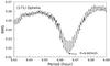 |
Fig. 1 Spin period distributions of (171) Ophelia vs. the rms values of the fits. |
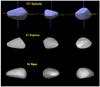 |
Fig. 2 Convex models of (171) Ophelia corresponding to the candidate pole 1 (top), (41) Daphne (middle), and (44) Nysa (bottom). For each asteroid, the three images are depicted 120° apart in rotational phase, the leftmost image corresponds to a view angle almost perpendicular to the longest axis. |
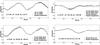 |
Fig. 3 Light curves of (171) Ophelia folded with the period of 6.665430 h. |
3.1. (171) Ophelia
For (171) Ophelia, 40 light curves obtained at six apparitions span 34 years, with the solar phase angle varying from  to 21°. Among these photometric data, the light curves at apparitions of 1979, 2005, and 2011 show the V-shaped minima. A range of the spin periods between 6.63 h to 6.69 h is scanned with a sampling step of 0.8Δp (with Δp defined according to Eq. (2) in Kaasalainenet al. 2001). In Fig. 1, it can be seen that the most significant minimum is around 6.66542 h. This period value is slightly smaller than that of Tedesco (1979). Setting this value as the new initial period, the fine shape, spin parameters, and the coefficient c are calculated. A pair of pole solutions are found at (149°, + 40°) and (333°, + 35°) in ecliptic coordinates (J2000) with comparable rms values of 0.012. For the two pole candidates, the spin periods are nearly the same, 6.665430 h. The weight coefficients c for the two poles are around 0.09. The shapes corresponding to the two poles are approximately mirror images of each other. The convex shape of (171) Ophelia (see Fig. 2) suggests a binary structure, which resembles the convex models of (41) Daphne and (44) Nysa (Kaasalainenet al. 2002b). The asteroid (171) Ophelia shows an elongated shape with one end clearly smaller than the other. The examples of observed light curves and modeled ones of (171) Ophelia are given in Fig. 3.
3.2. (360) Carlova
For (360) Carlova, 24 light curves obtained at eight apparitions are used in the shape inversion. The full data set spans 33 years (from 1979 to 2012), and the solar phase angle varies from 5° to 22°. With a similar procedure to that used for Ophelia, the best period value of 6.189592 h is found by scanning a wide range of periods, and then more homogeneous solutions of the shape and spin parmaters of (360) Carlova are derived with the convex inversion calculations. A pair of poles are found at (112°, 56°) and (335°,55°) with nearly the same rms values. The coefficients c for the two poles are 0.08 and 0.09, respectively.
To find the unique pole solution of Carlova, the occultation observation on August 15, 2011 (Dunhamet al. 2013), is used. Comparing the profile of Carlova derived directly from the event occulting TYC 0729-0057-1 to the projected profiles from our shape models in the same fundamental plane of occultation event of TYC 0729-0057-1 (see Fig. 4), we find that the shape model with the second pole (335°, + 55°) gives a very consistent profile to the occultation observation, while the shape mode with first pole (112°, + 56°) does not. The model shape of Carlova’s second pole is shown in the bottom left panel in Fig. 4.
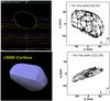 |
Fig. 4 Top left: profile of Carlova given by the event occulting TYC 0729-0057-1. Top and bottom right plots: projected profile of shape models at the same fundamental plane of the occultation event corresponding to pole 2 and 1, respectively. Bottom left: shape model of (360) Carlova. |
4. Uncertainties of the spin parameters
Kaasalainen et al. (2001) and Torppa et al. (2003) estimated the uncertainties of the pole and period by investigating the distribution of the parameters generated through varying the initial values of the parameters and the scattering models. Torppa et al. (2003) found that the distributions were usually steep, and the errors estimated from those distributions (e.g., typical errors of ±2° for the pole) are less realistic. In both studies, 0.01Δp − 0.1Δp were taken as the basic uncertainties of the spin period. Hanušet al. (2011) estimated the uncertainties of the spin parameters with the distribution of parameters generated by different “mock” objects, and gave a typical uncertainty of 10° for the pole.
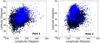 |
Fig. 5 Distributions of the pair poles of (171) Ophelia. The empty diamonds are the pole solutions of the fine shape model, and the crosses are of the coarse shape model. The big pluses are the corresponding mode values. |
Here, we utilize an approximate version of the MCMC-V method developed for asteroid orbital inversion by Muinonen et al. (2012) to estimate the uncertainties of spin parameters derived during the convex inversion. For the present inverse issue, the MCMC-V entails the following steps. Numbers of virtual photometric data sets are generated by adding Gaussian random noise to the original photometric data. The respective virtual least-squares solutions of convex inversion constitute a certain distribution of the unknown parameters. Convolution of this distribution by itself then provides a symmetric proposal distribution for a random-walk Metropolis-Hastings algorithm. A full MCMC treatment of convex inversion then follows and results in a joint distribution of the parameters. In the present context, we produce a preliminary error analysis of the spin parameters by using the virtual least-squares solutions, but omitting the final phase of MCMC-V. Because of this simplification, the resulting error bars are to be taken as indicative scale for the true errors, without strict probabilistic meaning in Bayesian inference.
To estimate the uncertainties of the spin parameters of (171) Ophelia and (360) Carlova, at least 5000 virtual photometric data sets are generated by adding random Gaussian noise into the observed brightness. The variance of Gaussian noise added in a light curve is set according to the standard deviation of fitting residuals to this light curve. It took nearly 17 h and 16 h to find the 1000 least-squares solutions using the convex inversion code for (171) Ophelia and (360) Carlova, respectively. From distributions of spin parameters composed of the virtual least-squares solutions (see Fig. 5, the case of Ophelia as the example), the most likely values and their uncertainties of model parameters are estimated by the mode value and the 1σ limits (the bounds between 15.85% and 84.15%) of the distributions. Table 1 lists the best values and uncertainties of spin parameters for the two asteroids.
Additionally, the effect of different resolution (six or eight triangulation rows when modeling shape) on the spin parameters is investigated by using the spin parameter distributions of Ophelia. We find that the pole distributions for shape models with different resolution (see Fig. 5) have similar coverage regions with slightly different mode values, while the distributions of period are the same. We prefer the pole solutions of the fine shape model because there is less rms of the observation data.
To understand the divergence of virtual convex shapes for a certain pole, the Pearson’s chi-square quantity, χ2, calculated from the facets’ area sizes of two of the virtual shapes (see Eq. (1)), is introduced to determine how similar the compared shape B is to the reference shape A: 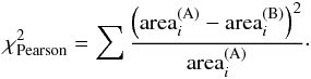 (1)For comparison, the facet sizes of a virtual shape are normalized by dividing by the sum of all the facets. A small value of χ2 reflects a strong similarity between the size distributions of two shapes. Each of the virtual shapes of a pole can be compared with the rest of shapes. The best shape is taken as the one that is similar to most of shapes. For example, the distribution of χ2 for the Ophelia pole 1 virtual convex shape shows a mode value of 2 and 90% of samples within χ2 of 12. What does χ2 of 12 mean? We calculate the Δρ (described in Eq. (5) of Kaasalainenet al. 2001) for two virtual shapes having a χ2 of 12, and find that it is less than 10%. Accordingly, we think a χ2 of 12 means a rough similarity between the two shapes.
Spin parameters and c of Ophelia and Carlova with uncertainties.
5. Summary
Using the convex inversion technique and the simplified MCMC-V method, the spin parameters, the Lambert law coefficient c and the shapes of (171) Ophelia and (360) Carlova have been derived.
Resembling the binary structures of (41) Daphne and (44) Nysa, the shape models of (171) Ophelia show binary structure. The approximate relative triaxial dimensions (Kaasalainenet al. 2002a) of (171) Ophelia are a/b = 1.22, a/c = 1.60, which show a flatter shape than that of (41) Daphne (a/b = 1.30, a/c = 1.47) and (44) Nysa (a/b = 1.33, a/c = 1.53; DAMIT, Ďurechet al. 2010). The unique pole (335°, + 55°) and the shape of Carlova are derived from the photometric data and occultation event. The unique pole is slightly different from the pole 2 of Ďurechet al. (2009) in longitude direction. The new shape looks like the Ďurechet al. (2009) shape model, but our model is flatter.
From the present analysis, the pole uncertainties for the two asteroids are about 4°–9°, and the uncertainties of the spin periods are less than 3 × 10⁻⁶ h. The pole uncertainties of (360) Carlova are larger than those of (171) Ophelia, which is in some measure due to the larger observational errors in parts of the photometric data of (360) Carlova.
IRAF is distributed by the National Optical Astronomy Observatories, which are operated by the Association of Universities for Research in Astronomy, Inc., under cooperative agreement with the National Science Foundation.
Acknowledgments
This work was supported by the National Natural Science Foundation of China (contracts Nos. 11073051 and 10933004) and the Academy of Finland (contract No. 127461). We would like to thank the Academy of Finland and the Chinese Academy of Sciences for providing financial support for the exchange visits enabling the present research. We are grateful to Mr. Tuomo Pieniluoma for valuable help with the visualization of the results.
References
- Di Martino, M., Zappalà, V., De Campos, J. A., Debehogne, H., & Lagerkvist, C.-I. 1987, A&AS, 67, 95 [NASA ADS] [Google Scholar]
- Dotto, E., De Angelis, G., & Di Martino, M. 1995, Icarus, 117, 313 [NASA ADS] [CrossRef] [Google Scholar]
- Dunham, D. W., Herald, D., Frappa, E., et al. 2013, Asteroid Occultations V11.0. EAR-A-3-RDR-OCCULTATIONS-V11.0, NASA Planetary Data System [Google Scholar]
- Ďurech, J., Kaasalainen, M., Warner, B. D., et al. 2009, A&A, 493, 291 [NASA ADS] [CrossRef] [EDP Sciences] [Google Scholar]
- Ďurech, J., Sidorin, V., & Kaasalainen, M. 2010, A&A, 513, A46 [NASA ADS] [CrossRef] [EDP Sciences] [Google Scholar]
- Hanuš, J., Ďurech, J., Brož, M., et al. 2011, A&A, 530, A134 [NASA ADS] [CrossRef] [EDP Sciences] [Google Scholar]
- Harris, A. W., & Young, J. W. 1983, Icarus, 54, 59 [NASA ADS] [CrossRef] [Google Scholar]
- Kaasalainen, M., & Torppa, J. 2001, Icarus, 153, 24 [NASA ADS] [CrossRef] [Google Scholar]
- Kaasalainen, M., Torppa, J., & Muinonen, K., 2001, Icarus, 153, 37 [NASA ADS] [CrossRef] [Google Scholar]
- Kaasalainen, M., Torppa, J., & Piironen, J., 2002a, Icarus, 159, 369 [NASA ADS] [CrossRef] [Google Scholar]
- Kaasalainen, M., Torppa, J., & Piironen, J. 2002b, A&A, 383, L19 [NASA ADS] [CrossRef] [EDP Sciences] [Google Scholar]
- Kaasalainen, S., Piironen, J., Kaasalainen, M., et al. 2003, Icarus, 161, 34 [NASA ADS] [CrossRef] [Google Scholar]
- Kaasalainen, M., Pravec, P., & Krugly, Y. N. 2004, Icarus, 167, 178 [NASA ADS] [CrossRef] [Google Scholar]
- Michalowski, T., Pych, W., Berthier, J., et al. 2000, A&AS, 146, 471 [NASA ADS] [CrossRef] [EDP Sciences] [Google Scholar]
- Muinonen, K., Granvik, M., Oszkiewicz, D., Pieniluoma, T., & Pentikäinen, H. 2012, Planet. Space Sci., 73, 15 [Google Scholar]
- Tedesco, E. F. 1979, Science, 203, 905 [NASA ADS] [CrossRef] [Google Scholar]
- Torppa, J., Kaasalainen, M., Michalowski, T., et al. 2003, Icarus, 164, 346 [NASA ADS] [CrossRef] [Google Scholar]
- Wang, X.-b., & Zhang, X-l. 2006, Chin. Astron. Astrophys., 30, 410 [NASA ADS] [CrossRef] [Google Scholar]
All Tables
All Figures
|
Fig. 1 Spin period distributions of (171) Ophelia vs. the rms values of the fits. |
| In the text | |
|
Fig. 2 Convex models of (171) Ophelia corresponding to the candidate pole 1 (top), (41) Daphne (middle), and (44) Nysa (bottom). For each asteroid, the three images are depicted 120° apart in rotational phase, the leftmost image corresponds to a view angle almost perpendicular to the longest axis. |
| In the text | |
|
Fig. 3 Light curves of (171) Ophelia folded with the period of 6.665430 h. |
| In the text | |
|
Fig. 4 Top left: profile of Carlova given by the event occulting TYC 0729-0057-1. Top and bottom right plots: projected profile of shape models at the same fundamental plane of the occultation event corresponding to pole 2 and 1, respectively. Bottom left: shape model of (360) Carlova. |
| In the text | |
|
Fig. 5 Distributions of the pair poles of (171) Ophelia. The empty diamonds are the pole solutions of the fine shape model, and the crosses are of the coarse shape model. The big pluses are the corresponding mode values. |
| In the text | |
Current usage metrics show cumulative count of Article Views (full-text article views including HTML views, PDF and ePub downloads, according to the available data) and Abstracts Views on Vision4Press platform.
Data correspond to usage on the plateform after 2015. The current usage metrics is available 48-96 hours after online publication and is updated daily on week days.
Initial download of the metrics may take a while.