| Issue |
A&A
Volume 581, September 2015
|
|
|---|---|---|
| Article Number | A46 | |
| Number of page(s) | 10 | |
| Section | Planets and planetary systems | |
| DOI | https://doi.org/10.1051/0004-6361/201526430 | |
| Published online | 01 September 2015 | |
Asteroid flux towards circumprimary habitable zones in binary star systems
I. Statistical overview
1 Institute of Astrophysics (ifA), University of Vienna, Türkenschanzstr. 17, 1180 Vienna, Austria
e-mail: This email address is being protected from spambots. You need JavaScript enabled to view it.
2 IMCCE, Paris Observatory, UPMC, CNRS, UMR 8028, 77 Av. Denfert-Rochereau 75014 Paris, France
3 Institut für Astronomie und Astrophysik, Eberhard Karls Universität Tübingen, Auf der Morgenstelle 10, 72076 Tübingen, Germany
4 Physikalisches Institut, Eberhard Karls Universität Tübingen, Auf der Morgenstelle 14, 72076 Tübingen, Germany
Received: 28 April 2015
Accepted: 29 June 2015
Abstract
Context. So far, more than 130 extrasolar planets have been found in multiple stellar systems. Dynamical simulations show that the outcome of the planetary formation process can lead to different planetary architecture (i.e. location, size, mass, and water content) when the star system is single or double.
Aims. In the late phase of planetary formation, when embryo-sized objects dominate the inner region of the system, asteroids are also present and can provide additional material for objects inside the habitable zone (HZ). In this study, we make a comparison of several binary star systems and how efficient they are at moving icy asteroids from beyond the snow line into orbits crossing the HZ.
Methods. We modelled a belt of 10 000 asteroids (remnants from the late phase of the planetary formation process) beyond the snow line. The planetesimals are placed randomly around the primary star and move under the gravitational influence of the two stars and a gas giant. As the planetesimals do not interact with each other, we divided the belt into 100 subrings which were integrated separately. In this statistical study, several double star configurations with a G-type star as primary are investigated.
Results. Our results show that small bodies also participate in bearing a non-negligible amount of water to the HZ. The proximity of a companion moving on an eccentric orbit increases the flux of asteroids to the HZ, which could result in a more efficient water transport on a short timescale, causing a heavy bombardment. In contrast to asteroids moving under the gravitational perturbations of one G-type star and a gas giant, we show that the presence of a companion star not only favours a faster depletion of our disk of planetesimals, but can also bring 4–5 times more water into the whole HZ.
Key words: celestial mechanics / methods: statistical / minor planets, asteroids: general / binaries: general
© ESO, 2015
1. Introduction
Nearly 130 extra solar planets in double and multiple star systems have been discovered to date. Roughly one quarter of these planets are orbiting close to or even crossing their systems’ habitable zone (HZ), i.e. the region where an Earth-analogue could retain liquid water on its surface (Rein 2014). While most of these planets are gas giants, the incredible ratio of one in four planets being at least partly in the HZ seems to make binary star systems promising targets in the search of a second Earth, especially for the next generation of photometry missions CHEOPS, TESS, and PLATO-2.0. About 80 percent (Rein 2014) of the currently known planets in double star systems are in so-called S-type configurations (Dvorak 1984), i.e. the two stars are so far apart so that the planet orbits only one stellar component without being destabilized. As most of the wide binary systems host more than one gas giant, their dynamical evolution is quite complex. The question whether habitable worlds can actually exist in such environments is, therefore, not a trivial one. Previous works on early stages of planetary formation show that planetesimal accretion can be more difficult than in single star systems (Thebault & Haghighipour 2014, and references therein). This in turn can question the possibility of whether embryos form in such systems. However, studies of late stages of planetary formation show that, should embryos manage to form despite these adverse conditions, the dynamical influence of companion stars is not prohibitive to forming Earth-like planets (Raymond et al. 2004; Haghighipour & Raymond 2007). Furthermore, it was shown that binary star systems in the vicinity of the solar system are capable of sustaining habitable worlds once they are formed (Eggl et al. 2013; Jaime et al. 2014). As the amount of water on a planet’s surface seems to be crucial to sustaining a temperate environment (Kasting et al. 1993), it is important to identify possible sources. For Earth, two mechanisms seem to be important: i) endogenous outgassing of primitive material; and ii) exogenous impact by asteroids and comets sources. Since neither can explain the amount of and isotope composition of Earth’s oceans in itself, models that favour a combination of both sources seem to be more successful (Izidoro et al. 2013). The amount of primordial water that is collected during formation phases of planets in S-type orbits in binary star systems containing additional gas giants has been studied by Haghighipour & Raymond (2007). They have shown that the planets formed in a circumstellar HZ may have collected between 4 and 40 Earth oceans from planetary embryos, but a main trend appeared: the more eccentric is the orbit of the binary, the more eccentricity is also injected into the gas giant’s orbit. This in turn leads to fewer and dryer terrestrial planets. Quintana et al. (2007) emphasize that during the late stages of planetary formation, without the presence of gas giant planets, binary stars with periastron >10 au have a minimal effect on terrestrial planet formation within ~2 au of the primary, whereas binary stars with periastron ≤5 au restrict terrestrial planet formation to within ~1 au of the primary star. Quintana & Lissauer (2006) studied the late stages of planetary formation in P-type orbits in binary star systems (with maximum separation equal to 0.4 au and the secondary’s maximum eccentricity equal to 0.8) including Jupiter and Saturn-like planets. They conclude that the higher the secondary’s apoapsis, the smaller the number of planets formed and the lower their mass. The anti-correlation between a system’s eccentricity and the number of planets has also been found in a preliminary interpretation of observation statistics by Limbach & Turner (2015). These results indicate that the likelihood of finding habitable planets in such an environment could be small.
Stochastic simulations proved that almost dry planets can also be formed in the circumprimary HZ of binary star systems (Haghighipour & Raymond 2007). However, as emphasized by these authors, water delivery in the inner solar system is not only due to radial mixing of planetary embryos. Smaller objects can also contribute as shown in Raymond et al. (2007). Indeed, they highlighted that water delivery from smaller planetesimals is statistically robust and should supply terrestrial planets with a significant water source of perhaps three to ten oceans. In our work, we aim to answer how much water can be transported into the HZ via small bodies, remnants from the late phase of the planetary formation, thus providing other water sources to embryos. We statistically study the dynamics of an asteroid belt in such systems and we treat this problem in a self-consistent manner as all the gravitational interactions in the system as well as water loss of the planetesimals due to outgassing are accounted for. Our main goal is to examine the influence of the secondary star on the flux of small bodies from icy regions to the HZ and the efficiency of the water transport within a short timescale of 10 Myr.
2. Initial conditions and dynamical model
Our study is focused on a primary G-type star with mass equal to one solar mass and we investigate the dynamical effect of a secondary of either G-, K-, or M-type with physical properties expressed in Table 1.
Physical properties of the secondary star in the binary system.
The studied binary star systems encompass relatively tight configurations, i.e. semi-major axes in the range of ab ∈ [25:100] au. This parameter has been changed in steps of 25 au in our simulations. The secondary is on an elliptical coplanar orbit with eccentricities eb ∈ [0.1:0.5] increased in steps of 0.2. In total 12 configurations have been investigated for any given stellar type of the companion. In addition, we consider a gas giant located at aGG = 5.2 au on a circular coplanar orbit, with a mass equal to Jupiter’s mass.
A disk of planetesimals is modelled as a ring of 10 000 asteroids with masses similar to main belt objects in the solar system and each asteroid was assigned an initial water mass fraction (hereafter wmf) of 10% (Abe et al. 2000; Morbidelli et al. 2000). During the late phase of planetary formation, if the inner region of the system is mainly dominated by large embryos (following a specific mass distribution) with masses between Moon and Mars sizes (Raymond et al. 2004; Haghighipour & Raymond 2007), debris resulting from collisions of such embryos are also present. To determine the lower and upper limits for the asteroids’ masses, we performed independent preliminary simulations with a 3D smooth particle hydrodynamics (SPH) code (Schäfer 2005; Maindl et al. 2013). First-order consistency is achieved by a tensorial correction as discussed in Schäfer et al. (2007). It includes self-gravity and models material strength using the full elasto-plastic continuum mechanics and the Grady-Kipp fragmentation model for fracture and brittle failure (Grady & Kipp 1980; Benz & Asphaug 1994). The scenarios involve collisions of rocky basaltic objects with one lunar mass at different encounter velocities and angles α. The latter are defined in a way so that α = 0° corresponds to a head-on collision. The scenarios start with the bodies five diameters apart to let the SPH particle distribution settle. This preliminary simulation time span was 2000 min. In an earlier study, most collisions of Moon-sized bodies in the solar system’s HZ were found to happen at velocities v ≲ 2 vesc at arbitrary collision angles (Maindl & Dvorak 2014). We chose initial conditions in this range which are in the merging/partial accretion and hit-and-run domain of the collision outcome map (cf. Agnor & Asphaug 2004; Leinhardt & Stewart 2012; Maindl et al. 2014). Expecting a somewhat higher spread in v in binary systems we also included a scenario in the erosion/mutual destruction domain. Table 2 lists the collision scenario parameters and gives the resulting mass loss of the survivors (one body for merging, two bodies in both the erosion and the hit-and-run scenarios) after one impact.
Mass loss in the simulated collisions.
 |
Fig. 1 Collision scenarios resulting in a merge a), a hit-and-run encounter b), and erosion/mutual destruction c). The diagrams show the masses of the ten largest fragments at the end of the simulation as percentages of the total system mass Mtot = 2 lunar masses. The dashed horizontal line indicates the limit for significant fragments (see text). |
The fragment sizes beyond the survivors drop significantly in the hit-and-run and merging scenarios (Figs. 1a,b): in the mutual destruction case, all of the ten largest fragments possess masses ≳1% of the total system mass, which is approximately Ceres’ mass1, and hundreds are above the “significant” fragment threshold in the sense of Maindl et al. (2014). The smallest fragment consists of one SPH particle (0.001% of the total mass for 100 k SPH particles) which corresponds to ~0.1% of Ceres’ mass. As increasing the number of SPH particles will result in even smaller fragments, this mass is an upper limit for the smallest fragment. As this fragment will contain ~0.006% Earth-oceans units2, we chose to neglect the water contribution of smaller particles. Our minimum and maximum mass are thus defined according to the fragments’ mass after one impact. Therefore, members of our ring will have masses randomly and equally distributed between 0.1% to one Ceres’ mass. The total mass of the ring of 10 000 asteroids amounts to MR = 0.5 M⊕. Thus, the quantity of water in terms of Earth-ocean units available in a ring will be 200.
In each system, we defined the size of the disk of planetesimals by the following borders. As we focus on the transport of icy bodies, the inner border of the disk is set to the snow line position (Lecar et al. 2006; Martin & Livio 2012, 2013), the border between icy and rocky planetesimals. Its position changes as the star’s luminosity evolves during its birth phase. As our host star is a G2V type, we considered the inner border of the disk of planetesimals according to observations in the solar system that suggest that the snow line is at ~2.7 au. The outer border of the disk of planetesimals is influenced by perturbations induced by the secondary star. Since we consider initially circular motion for the planetesimals, the stability border depends mainly on three parameters: the mass ratio of the system, ab, and eb (Rabl & Dvorak 1988; Holman & Wiegert 1999; Pilat-Lohinger & Dvorak 2002). These authors showed that it is possible to link these parameters to derive a critical semi-major axis ac as the maximum initial semi-major axis for a particle to survive in the system. In contrast to Rabl & Dvorak (1988) and Holman & Wiegert (1999) who classified unstable orbits via ejections of test planets from the system, Pilat-Lohinger & Dvorak (2002) calculated the Fast Lyapunov Indicator (FLI) for each orbit to distinguish between stable and chaotic motion. This well-known chaos detection method was introduced by Froeschlé et al. (1997). In the case of circular motion of the planets and the planetesimals, it is possible to use the study by Holman & Wiegert (1999) where ac and its uncertainty Δac allows a good determination of the outer border (maximum semi-major axis allowed) for asteroids in the ring as ac − Δac, which is in good agreement with the stability limits derived from FLI computations (Pilat-Lohinger & Dvorak 2002). Asteroids in our belt are randomly positioned between the inner (the snow line) and and outer borders (the stability limit ac − Δac). Figure 2 shows a comparison of initial mass distribution of asteroids for a secondary M star at 100 au and eb = 0.1 and 0.5. The position of the gas giant planet is indicated by the vertical line. Because of the binary’s tight periapsis in the case of eb = 0.5, the asteroid belt is less extended and exhibits a higher mass density. In order to prevent immediate dynamical instability, all bodies were carefully placed so that their initial mutual separations were at least several Hill’s radii.
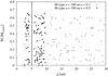 |
Fig. 2 Example of mass distributions in the circumprimary ring as a function of the asteroids’ semi-major axis under the gravitational influence of a secondary M star at ab = 100 au and eb = 0.1 (■) and eb = 0.5 (•). The vertical line refers to the gas giant’s position. All particles are initially spaced by several Hill’s radii to prevent immediate dynamical instability. |
In our main simulations, as we assume that the giant planet is already formed so that the remaining gas has evaporated or coagulated into the asteroid belt, we do not take any effects related to gas drag into account (therefore no gas driven migration, no eccentricity dampening). The initial eccentricities and inclinations are randomly chosen below 0.01 and 1° respectively. To avoid strong initial interactions with the gas giant, we assume that the giant planet has cleared a path in the disk around its orbit. The width of this gap is ±3 RH,GG, where RH,GG is the giant planet’s Hill Radius3. Requiring orbital stability of the gas giant at 5.2 au reduces the number of possible binary configurations. Therefore, we excluded the case where ac − Δac ≤ aGG + 3 RH,GG. This results in a total number of 23 binary systems configurations that were studied in this work; they are summarized in Table 3.
Binary configurations studied in this article.
We limited our study to 10 Myr integration time. This is of course much shorter than the timescale of terrestrial planetary formation (~100 Myr), but as we make a comparison of many different binary star systems, we had to restrict this study to a shorter time. However, we will select from this study the most interesting systems for which a statistic over 100 Myr will be made. We numerically integrated our systems using the nine package (Eggl & Dvorak 2010) and only gravitational perturbations were taken into account. The numerical integrator used for the computations is based on the Lie-series (see e.g. Hanslmeier & Dvorak 1984 and more recently Bancelin et al. 2012). For a given configuration in Table 3, as our planetesimals do not interact with each other, the disk was divided into 100 subrings and separately integrated.
3. The habitable zone
As we study the flux of water-rich asteroids into the HZ, we need to know the position of this area. The definition, modelling, and computation of the “classical HZ” (hereafter CHZ) is given in Kasting (1988, 1991), Kasting et al. (1993), and Kopparapu et al. (2013). All these studies are based on a 1D cloud-free climate model, where the inner edge of the HZ is computed by increasing the surface temperature and the outer edge by increasing the CO2 partial pressure (maintaining a constant surface temperature at 273 K). The corresponding stellar flux needed to maintain the surface temperature is then derived. Thus, these authors were able to express the CHZ borders as a simple fit function containing the stellar luminosity and temperature. Recently, Kopparapu et al. (2014) investigated the dependence of the HZ borders on the planetary masses and derived new coefficients for the computations of the effective solar flux. For a G star, the inner edge of the HZ corresponding to the runaway greenhouse limit is 0.950 au and the outer edge of the HZ corresponding to the maximum greenhouse is 1.676 au. The updated inner edge value is closer to the Sun than the one found by Kopparapu et al. (2013) because they used inputs from a 3D model by Leconte et al. (2013). However, the exact value for the inner CHZ border depends on many assumptions and is still under discussion in current literature, (e.g. Wolf & Toon 2014).
When including a binary companion in the system, the additional gravitational interaction and radiation can shrink the CHZ borders, as shown in Eggl et al. (2012) and Kaltenegger & Haghighipour (2013). Actually, the smaller the periapsis of the binary, the more important the insolation of the primary, as the periapsis distance of the planet with respect to its host star can change significantly. In order to account for this effect, Eggl et al. (2012) introduced the so-called permanently habitable zone (hereafter PHZ). The PHZ contains information on the planet’s perturbed orbit. It serves as a way to distinguish areas where a planet always receives the correct amount of insolation to remain habitable from regions where insolation conditions for habitability are only fulfilled in an average4 sense. Figure 3 shows the ratio PHZ/CHZ as a function of the binary’s orbital elements (ab, eb) for a G2V-G2V binary star system. The blue and black colours cover a large region where no or only minor differences between PHZ and CHZ were found. This means that the additional radiation from the second star is not enough to drastically cause a change of insolation at the surface of a planet because the secondary is too far or its periapsis too far away. For higher eccentricities where the secondary’s orbit approaches closer to the host star, the difference increases (green). The red colour refers to regions where the PHZ vanishes either due to excessive insolation or due to orbital instability. It is clear that the truncation of the PHZ increases for large values of the periapsis of the binary companion. This occurs because the stellar gravitational perturbations acting on the planet will cause a significant change of the planet’s periapsis, which in turn influences the insolation at the planet’s surface. A similar behaviour is observed for K and M class secondaries as their mass does not significantly influence the PHZ/CHZ ratio. For our binary configurations, the difference between CHZ and PHZ is only of the order of 10% as shown in Table 4. As these values do not vary strongly with the secondary’s mass, we did not list all 23 configurations.
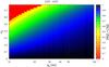 |
Fig. 3 PHZ/CHZ ratio as a function of the binary separation and the secondary’s eccentricity. The red colour indicates that the planet will always lie outside the PHZ borders. Only a graph for a secondary G star is represented as it is quite similar for a secondary K and M-types. |
4. Asteroid flux and water transport to the HZ
4.1. Statistics on the disk dynamics
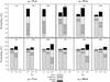 |
Fig. 4 Statistics on the disk of planetesimals dynamics. Each histogram shows the evolution (expressed in probability) of the asteroids in the ring within 10 Myr of integration. They can still be present in the system (“alive”), become a HZc, collide with the stars or the gas giant, or be ejected out of the system. The closer the secondary and the higher its mass, the higher the probability to empty the asteroids ring. |
During the simulation, each particle is tracked until the end of the integration time in order to assess the following numbers:
-
Asteroids crossing the HZ. They will be referred to as habitablezone crossers5(hereafter HZc). As we assume a two-dimensional HZ, anasteroid will be considered a HZc if the intersection point betweenits orbit and the HZ plane lies within the HZ borders.
-
Asteroids leaving the system when their semi-major axis ≥500 au.
-
Asteroids colliding with the gas giant or the stars.
-
Asteroids still alive in the belt after 10 Myr.
Figure 4 shows the resulting statistics on the asteroids’ dynamics, each of the four panels corresponding to the secondary’s semi-major axis. Each histogram shows the dynamical outcome of our asteroids expressed in terms of probability, as a function of the secondary’s eccentricity. Below 100%, the percentage of asteroids that are still present in the belt (“alive”), that were ejected or that collided with the stars or the gas giant is shown. The black area of each histogram above 100% indicates the probability that asteroids will enter the HZ. Such asteroids, crossing the HZ, are called HZc. The perturbations due to both the gas giant and the binary companion can cause an increase in eccentricity of the asteroids within the planetesimal disk, which of course depends on the binary configuration. A comparison of the different histograms indicates that the most important parameter is the periapse of the binary system, which is defined by the eccentricity of the binary. Of course, not only the asteroids are perturbed by the secondary; the gas giant at 5.2 au is also perturbed and its initially circular motion will change to an elliptic one. This behaviour is highlighted by the increasing value of the probability of becoming a HZc if the secondary’s periapsis distance decreases and if its mass increases. Indeed, for a given value of ab (for instance 50 au), one can see that this probability is at least doubled when eb increases. As a consequence, the asteroid belt will be depopulated because of dynamically induced ejections, as well as collisions with the giant planet and the stars. Because the rate of colliding and ejected asteroids is higher, a ring will be depopulated faster when eb becomes larger. Therefore, the statistics in Fig. 4 shows that the probability of a member of the asteroid ring staying in the system after 10 Myr will decrease with the periapsis distance and the secondary star’s mass. Finally, these results can also answer the question of the presence of an asteroid belt in such systems. Indeed, if we assume that the gas could protect small bodies from secular resonances or mean motion resonances (MMRs), it is highly unlikely that they can survive in binaries with small periapsis separation after the gas has dissipated.
PHZ borders given in au as a function of the binary orbital characteristics (ab, eb) used in our simulations.
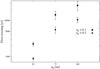 |
Fig. 5 Median time for an asteroid to become a HZc for the case of a secondary G-type with eb = 0.1 (■) and eb = 0.3 (•). This corresponds to the time when an asteroid crosses the HZ for the first time. The statistics is made over the 10 000 asteroids and the 1σ value is represented by error bars. |
4.2. Timescale statistics
Depending on the periapsis distance of the secondary, the disk of planetesimals can be perturbed more or less rapidly. Asteroids will suffer from the gravitational perturbations of the secondary star and the gas giant, and their eccentricity may increase quickly. Figure 5 shows the statistical results of the average time needed by an asteroid to become a HZc, i.e. the time it takes to reach the HZ. This corresponds to the time spans until the first asteroid enters the HZ. The median value and its absolute deviation (error bars) are presented for a set of 10 000 asteroids for the case of a secondary G-type with eb = 0.1 (■) and eb = 0.3 (•). This confirms a strong correlation between the periapsis distance and the time of first crossing. Figure 5 clearly shows that the average time varies from a few centuries to tens of thousands of years. The closer and more massive the secondary star, the sooner asteroids can reach the HZ. In contrast, the crossing timescale will become larger as the number of HZc increases as shown in Fig. 6. This parameter corresponds to the bombardment timescale, within 10 Myr of integration time, and is derived considering the last crossing inside the HZ, but not the asteroid’s water content. Indeed, once an asteroid becomes a HZc, it can cross the HZ several times as long as its orbit is stable and until it is ejected out of the system or collides with the giant planet or the stars. However, water-rich asteroids could be dry before this corresponding timescale, revealing that water transport could occur on a very short timescale (compared to planetary formation timescale). In addition, it can be seen in Fig. 6 that most of the systems, with large ab and low eb, having low crossing timescales are also those where most asteroids remained in the system after 10 Myr as shown in Fig. 4. This suggests that asteroid flux to the HZ could occur in several steps as some asteroids need more time to drastically increase their eccentricity in order to be moved to lower orbits and reach the HZ. This also reveals that water sources can still be available in the ring, provided that asteroids still have icy water on their surface. This study would of course require longer integration time (>10 Myr). Nevertheless, we have a clear indication of the efficiency with which binary stars systems transport asteroids from beyond the snow line to the HZ on a short timescale.
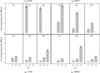 |
Fig. 6 Crossing timescale expressed in Myr. It corresponds to the last crossing inside the HZ. Up to 6 Myr for the most perturbed systems but also with the lowest number of asteroids still present in the system within 10 Myr of integration time. For the other systems, the crossing timescale is much lower because their belt still contain a huge number of “alive” asteroids. Indeed, the dynamics of the system needs more time to empty the asteroid belt population. |
4.3. Water transport statistics
Each HZc entering the HZ will bring a certain amount of water. However, regarding the integration timescale, the water content of asteroids may vary with time. Indeed, increased eccentricities can cause asteroids to approach close to the stars. This in turn would lead to a mass variation mainly due to a loss of their water content.
4.3.1. Water mass loss process
To quantitatively assess the water content of asteroids, we followed their water mass fraction evolution throughout the simulations, including the mass loss process, until they enter the HZ. The main mechanisms that can induce a relevant mass loss for active (comet-like) or inactive asteroids are ice sublimation and impact ejection (Jewitt 2012). The latter process occurs when smaller asteroids impact larger ones6. These impacts can be highly erosive due to characteristic speeds ~5 km s-1 (Bottke et al. 1994) and the amount of ejected mass can be significant. However, typical impact events in the main-belt have an impact probability ~3.0 × 10⁻⁸ km-2 yr-1 (Farinella & Davis 1992). However, according to Bottke et al. (2005), the timescale for an impact event to happen in our sample of asteroids belt (with radius from tens to hundreds of kilometers) is much longer than our integration time. Thus, we neglected this process in our study. The only mass loss process we consider is due to ice sublimation when the asteroid comes relatively close to the star. This process can be stepped up in double star systems, especially when the companion is on an eccentric orbit. Even if the secondary is not particularly close, the asteroid’s eccentricity can be pumped and it can receive a large amount of insolation. Therefore, the water mass loss rate ṁ was computed accounting for the radiation of both stars. The estimation of ṁ can be derived by solving a balance energy equation between the net incoming stellar flux, the ice sublimation and the thermal re-radiation7, as expressed in Eq. (1), ![Mathematical equation: \begin{eqnarray} \label{E:energy} \sum_{i\,=\,1}^2 \frac{{F}_{\star,{i}}(1-\text{A}_{i})}{{R}^{ 2}_{ {i}} [\text{au}]}\cos{\theta}_{ {i}} = \epsilon \sigma {T}^{ 4} + {L(T)}\,\dot{m} {(T)}, \end{eqnarray}](/articles/aa/full_html/2015/09/aa26430-15/aa26430-15-eq49.png) (1)where
(1)where
-
F⋆ is the stellar constant and is computed as F⋆ = F⊙L⋆ (F⊙ ~ 1360 W m-2 is the solar constant);
-
−
A, the bound albedo, product of the geometric albedo and the phase integral, defines the fraction of the total incident stellar radiation reflected by an object back to space. Asteroids can have A ≃ 0.5, but most of them have relatively low albedo (Shestopalov & Golubeva 2011). Ice material is known to be a good radiation reflector. In order to maximize ṁ, we follow the approach of Jewitt (2012) and we consider our objects with dirty ice material with low albedo because clean ice sublimates too slowly at main-belt distances. Therefore, we used an averaged albedo
 ;
; -
R is the distance to the star (primary or secondary) expressed in au;
-
θ is the angle between the incident light and the normal to the asteroid’s surface. According to Jewitt (2012), ṁ is weaker for an isothermal surface than at the subsolar point of a non-rotating body. Again, to maximize ṁ, we consider the subsolar case with θ = 0°;
-
ϵ is the emissivity of the surface, ϵ ~ 0.9;
-
σ = 5.67 × 10⁻⁸ W m-2 K-4 is the Boltzmann constant;
-
T is the equilibrium temperature at the surface expressed in K;
-
L is the latent heat of sublimation in J kg-1;
-
ṁ is the surface mass loss rate in kg m-2 s-1.
Here ṁ can be obtained by computing the temperature T solving Eq. (1). To this purpose, we expressed all the variable parameters as a function of T. According to Delsemme & Miller (1971), ṁ can be written as 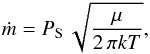 (2)where μ = 18 g mol-1 is the water molar mass and PS is the saturation pressure and is defined by the empirical formula
  (3)Finally, the latent heat is expressed as
  (4)
(4)
4.3.2. The water mass fraction of incoming HZc
The value of ṁ is constantly updated during the simulations and the accumulated surface mass loss dm reads  (5)where Δt represents the time elapsed since the beginning of the integration. We then compute the sublimating area 4πr2 with r the radius of the HZc. If we consider the following density for water ice shell and a basalt core, respectively ρi = 900 kg m-3 and ρc = 3000 kg m-3, then for a given wmf, the mean density of an asteroid is
  Therefore,
 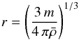 with m the mass of the asteroid. Thus, we can derive the total water mass loss in kg Δ m = dm × 4πr2.
Whenever an asteroid becomes a HZc, i.e. when it first enters the HZ, we suppose that its current water content will be delivered. This is the best-case scenario because the total water content of the HZc corresponds to the maximum amount of water available in the HZ. In reality, however, only a small fraction of water would be accreted onto a planet (or planetary system) inside the HZ. Indeed, both the real position of the planet on its orbit and the impact velocity of these HZc are crucial parameters in collisional material transport as pointed out by Thébault et al. (2006) and Leinhardt & Stewart (2012). A fully self-consistent modelling of the water delivery at impact lies beyond the scope of the current work, however. We aim to study the amount of water transported into the HZ rather than the amount of water accreted by a planet there. Figure 7 shows the total amount of water that was transported into the HZ (expressed in terrestrial oceans units) as a function of the binary system characteristics. Each histogram represents the total number of oceans ending in four partitions of the HZ. They correspond to equally spaced rings using the values obtained in Table 4. Therefore, we define the inner HZ border (closest ring to the PHZ inner border value), Central 1 and 2 (intermediate borders), and Outer HZ (closest ring to the PHZ outer border value). Also illustrated in this figure is the additional quantity of water transported between the inner edge A [CHZ(A); PHZ(A)] and the outer edge B [PHZ (B); CHZ(B)] of the HZ (in grey and labelled “additional”).
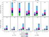 |
Fig. 7 Total number of oceans transported by all the HZc when they first cross the HZ. The colour code is related to four equally spaced rings of the HZ: inner, central 1 and 2, outer HZ (see text). We also indicated the equivalent number of additional oceans crossing the truncated CHZ interval when the dynamics of the secondary star is not taken into account for the computation of the HZ borders. |
The main results suggested by this figure are the following:
-
a)
A maximum of 70 oceans can be transportedinto the CHZ. We note that 70 oceans repre-sents 35% of the total number of oceans containedin the 10 000 asteroids pop-ulation8. Variancesare large, however. One of the reasons for the wide spread in theamount of transported water is the short simulation time. This in-troduces a bias towards systems where the water transport is fast.In other words, the seemingly small amount of transported waterin some of the presented systems does not imply that their HZshave to remain dry. It merely highlights the fact that the deliveryprocess would require a longer time, as many asteroids are stillpresent in the system after 10 Myr of integrationtime (see Fig. 4). However, these results show howfast and efficient some systems are at transporting water.
-
b)
The difference between the water transported in CHZ and PHZ (grey) is not that significant compared to the total number of incoming oceans. Indeed, the difference does not exceed ~3 oceans. One should note that we disregarded large orbital variations of any embryos located in the HZ caused by the perturbed motion of the gas giant because of the presence of the secondary star. This in turn can perturb the motion on any planets in the HZ9. However, according to Williams & Pollard (2002), an average insolation – covering almost the entire CHZ – is sufficient to retain liquid water on an Earth-twin surface and secure the habitability of planets.
-
c)
Any binary star system is efficient enough to produce a flux of asteroids within the whole HZ and thus to make water sources available for embryos lying there. However, we can see that statistically, most of the water ends up in the outer HZ. This occurs because its surface area is much wider than the other rings and the probability of an asteroid falling in the outer HZ is higher. The quantity of water brought into the outer HZ versus the other cells is quite balanced. Indeed, regarding the definition of a HZc, we do not expect asteroids on inclined orbits to necessarily cross the outer HZ. In addition, dynamical studies suggest that secular perturbations can lie inside the HZ or beyond the snow line, depending on a binary system’s characteristics (Bancelin et al., in prep.; Baszó et al., in prep.; Pilat et al., in prep.). In addition, depending on the secondary’s periapsis, the secondary will shorten the lifetime of particles inside MMRs (Bancelin et al., in prep.). Therefore, for asteroids initially orbiting inside MMRs and/or secular perturbations, the dynamical evolution can be violent and their orbit crossing the HZ will not necessarily be from the outer HZ to the inner HZ.
4.4. Influence of the initial water content
We now compare the water transport efficiency when the initial wmf is not equally distributed throughout the asteroid belt. The equal water distribution model is called WMFA. Observations in the main-belt (Abe et al. 2000; DeMeo & Carry 2014) suggest that a gradient exists in the chemical composition of the asteroids. In addition, we expect distant asteroids, up to the Kuiper-belt distance, to have a higher wmf than asteroids in the main-belt. Thus, we modelled the wmf distribution (called WMFB) as a linear function of the distance to the central star, fulfilling the following boundary conditions: the upper limit is fixed at 20% of water for asteroids at 30 au10. To find the lower limit for asteroids at 2.7 au, we follow Raymond et al. (2004) and Haghighipour & Raymond (2007) assuming a wmf ~5%. Under these assumptions, a belt in tight binary systems will have a lower water mass ratio than a belt under the influence of a secondary on a low eccentric orbit. Indeed, the ratio between model WMFB and WMFA gives lower limits of 0.62, 0.58, and 0.63 respectively for G, K, and M secondary stars. When the secondary’s periapsis increases, we get upper limits of 1.07, 1.18, and 1.27, respectively. However, the number of oceans transported to the HZ using WMFB does not exceed two-thirds of the amount of transported water when using WMFA, even if the belt initially contains more water. This shows that
-
a)
our results are robust;
-
b)
asteroids closer to the snow line are more likely to become HZc. According to model WMFB, asteroids will contain 10% of water if they are located below 11 au11. If asteroids becoming HZc were initially beyond this distance, we would have an equivalent or higher number of transported oceans.
5. Comparison with a single G-star system
In this section, we will compare the water transport efficiency between binary and single star systems. To this purpose, we considered the same initial conditions for the gas giant and the asteroid belt distribution, except that we only have a single G star in our dynamical system. As the comparisons are made for the same initial conditions of the asteroids, we have to consider, for the single star system, the same size for the disk given by the binaries’ characteristics, which is why the results for the reference single star case are different depending on the values of the binary’s eccentricity and separation (see Fig. 9).
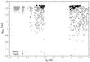 |
Fig. 8 Initial semi-major axis a0 and final periapsis distance qHZc of the incoming HZc for a single (•) and binary (■) star system. |
For computational reasons, our comparison is limited to a G2V-G2V-type binary. In addition, there are no more crossings in the HZ after 5–6 Myr (Fig. 6). Therefore, the number of oceans brought to the HZ will not vary after this time. Thus, each system was compared at equivalent integration times (≤5 Myr). Our results show that an asteroid that was initially in the ring will need 2–20 times longer to reach the HZ in a single star system. In other words, because the asteroid belt is not perturbed strongly enough by the gas giant to produce a large asteroid flux towards the HZ (Fig. 8), the presence of the secondary star can put asteroids with initial semi-major axis a0 on high eccentric orbits, i.e. very low periapsis distance qHZc. This will result in a faster depletion of the belt and a shorter bombardment duration than in a single star system.
Consequently, the probability of an asteroid crossing the HZ will be ~4–6 times higher in a binary star system. We note that the number of scattered incoming asteroids mainly increases because the secondary star perturbs the giant planet’s orbit. As the flux of asteroids is less efficient in a single star system, the amount of water brought to the HZ is smaller. In fact, the water transport is 4–5 times less efficient without a second star.
Finally, Fig. 9 compares the amount of delivered water in various systems. The histograms marked with the letter B refer to binary star systems, those with the letter S to single star systems. The colour code indicates the amount of water that ended up in four equally spaced subrings (Inner, Central 1, Central 2, Outer) of the corresponding PHZ (see Table 4). For a single star system, each ring of the CHZ is computed using the inner edge value 0.950 au and outer edge value 1.676 au. It is not surprising that the outer HZ is the most crossed ring. Indeed, its area is much larger than the other rings. This figure also highlights the fact that in such single star systems that host only one giant planet, basically all the water is transported in the outer HZ because the perturbation is not strong enough to drastically increase the eccentricity of any asteroid in the belt. These results show the efficiency with which a binary star transports water in the entire HZ over a shorter timescale compared to a single star system.
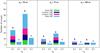 |
Fig. 9 Comparison of the water transport in single star (S) and binary star (B) systems. We restricted this study to binaries with two G-type stars. The various panels correspond to different semi-major axes of the secondary: ab = 50–75–100 au. The colour code refers to different subrings of the HZ (see text). We note that the two results for each panel account for different initial asteroid belt distributions (depending on eb), taken as the same for (S) and (B). |
6. Summary and conclusion
In this work, we investigated the influence of a secondary star on the flux of asteroids to the habitable zone (HZ) over 10 Myr of integration time. We estimated the quantity of water brought by asteroids located beyond the snow line into the HZ of various double star configurations (separation, eccentricity, and mass of the secondary). An overlap of perturbations from the secondary and the giant planet in the primordial asteroid belt causes rapid and violent changes in the asteroids’ orbits. This leads to asteroids crossing the HZ soon after the gas in the system has dissipated and the gravitational dynamics become dominant. Our results point out that binary systems are more efficient at transporting water into the HZ than a single star system. Not only is an asteroid’s flux 4–6 times higher when a secondary star is present, but the number of transported oceans to the HZ can also be 4–5 times higher, providing other water sources to embryos, in the whole HZ, in the late phase of planetary formation. Our results stress the fact that some systems can complete their water transport in a short time (~6 Myr), in contrast to single star system. Finally, our study can give a clear idea of the dynamics and the stability of objects moving under the perturbations of a binary star system and a gas giant. Indeed, as the depletion of an asteroid belt in binaries with small periapsis separations is faster, only a few small bodies will remain members of this belt. Thus, it would be unlikely to observe such an asteroid belt in such systems.
It is clear that dynamics in single and binary systems are completely different as the presence of the secondary together with a gas giant would have a direct impact on the dynamics of an asteroid belt, but also on any planets or embryos located in the HZ. Indeed, similarly to the work of Pilat-Lohinger et al. (2008), secular perturbations and MMRs’ intensity depend on the secondary’s orbital parameters and mass, which will be the subject of a future study.
Ceres’ mass is equal to 4.73 × 10⁻¹⁰M⊙.
1 ocean = 1.5 × 10²¹ kg of H2O.
However, we did not exclude possible location of asteroids inside mean motion resonances (MMRs). Indeed, we assume that the presence of the gas might have kept asteroids on stable orbits inside MMRs. Then, the MMR perturbations became stronger when the gas vanished.
The planet’s orbit is eccentric enough that it could leave the HZ from time to time.
A HZc can cross the HZ several times before leaving the system or colliding with the stars or the planets.
Such impacts do not necessarily lead to a complete destruction or break-up of asteroids.
Assuming the asteroid to have black-body properties.
200 oceans contained in this population.
When including a gas giant in a binary star systems, its additional perturbation will increase the eccentricity on any planets located in the HZ.
As shown in Fig. 2, our objects’ semi-major axis does not go beyond 30 au.
Provided that the critical semi-major axis criteria allows asteroids to be located beyond this distance.
Acknowledgments
D.B., E.P.L., T.M. and R.D. acknowledge the support of the FWF NFN project: “Pathways to Habitability” and related subprojects S11608-N16 “Binary Star Systems and Habitability” and S11603 “Water transport”. D.B. and E.P.L. also acknowledge the Vienna Scientific Cluster (VSC project 70320) for computational resources. S.E. has been supported by the European Union Seventh Framework Program (FP7/2007-2013) under grant agreement No. 282703.
References
- Abe, Y., Ohtani, E., Okuchi, T., Righter, K., & Drake, M. 2000, in Origin of the earth and moon, eds. R. M. Canup, K. Righter, et al., 413 [Google Scholar]
- Agnor, C., & Asphaug, E. 2004, ApJ, 613, L157 [NASA ADS] [CrossRef] [Google Scholar]
- Bancelin, D., Hestroffer, D., & Thuillot, W. 2012, Celest. Mech. Dyn. Astron., 112, 221 [NASA ADS] [CrossRef] [Google Scholar]
- Benz, W., & Asphaug, E. 1994, Icarus, 107, 98 [NASA ADS] [CrossRef] [Google Scholar]
- Bottke, W. F., Nolan, M. C., Greenberg, R., & Kolvoord, R. A. 1994, Icarus, 107, 255 [NASA ADS] [CrossRef] [Google Scholar]
- Bottke, W. F., Durda, D. D., Nesvorný, D., et al. 2005, Icarus, 179, 63 [NASA ADS] [CrossRef] [Google Scholar]
- Delsemme, A. H., & Miller, D. C. 1971, Planet. Space Sci., 19, 1229 [NASA ADS] [CrossRef] [Google Scholar]
- DeMeo, F. E., & Carry, B. 2014, Nature, 505, 629 [NASA ADS] [CrossRef] [Google Scholar]
- Dvorak, R. 1984, Celest. Mech., 34, 369 [NASA ADS] [CrossRef] [Google Scholar]
- Eggl, S., & Dvorak, R. 2010, in Dynamics of Small Solar System Bodies and Exoplanets, eds. J. Souchay & R. Dvorak (Berlin: Springer Verlag), Lect. Note Phys. 790, 431 [Google Scholar]
- Eggl, S., Pilat-Lohinger, E., Georgakarakos, N., Gyergyovits, M., & Funk, B. 2012, ApJ, 752, 74 [NASA ADS] [CrossRef] [Google Scholar]
- Eggl, S., Pilat-Lohinger, E., Funk, B., Georgakarakos, N., & Haghighipour, N. 2013, MNRAS, 428, 3104 [NASA ADS] [CrossRef] [Google Scholar]
- Farinella, P., & Davis, D. R. 1992, Icarus, 97, 111 [NASA ADS] [CrossRef] [Google Scholar]
- Froeschlé, C., Lega, E., & Gonczi, R. 1997, Celest. Mech. Dyn. Astron., 67, 41 [CrossRef] [Google Scholar]
- Grady, D. E., & Kipp, M. E. 1980, International Journal of Rock Mechanics and Mining Sciences & Geomechanics Abstracts, 17, 147 [Google Scholar]
- Haghighipour, N., & Raymond, S. N. 2007, ApJ, 666, 436 [NASA ADS] [CrossRef] [Google Scholar]
- Hanslmeier, A., & Dvorak, R. 1984, A&A, 132, 203 [NASA ADS] [Google Scholar]
- Holman, M. J., & Wiegert, P. A. 1999, AJ, 117, 621 [NASA ADS] [CrossRef] [Google Scholar]
- Izidoro, A., de Souza Torres, K., Winter, O. C., & Haghighipour, N. 2013, ApJ, 767, 54 [NASA ADS] [CrossRef] [Google Scholar]
- Jaime, L. G., Aguilar, L., & Pichardo, B. 2014, MNRAS, 443, 260 [NASA ADS] [CrossRef] [Google Scholar]
- Jewitt, D. 2012, AJ, 143, 66 [NASA ADS] [CrossRef] [Google Scholar]
- Kaltenegger, L., & Haghighipour, N. 2013, ApJ, 777, 165 [NASA ADS] [CrossRef] [Google Scholar]
- Kasting, J. F. 1988, Icarus, 74, 472 [NASA ADS] [CrossRef] [PubMed] [Google Scholar]
- Kasting, J. F. 1991, Icarus, 94, 1 [NASA ADS] [CrossRef] [Google Scholar]
- Kasting, J. F., Whitmire, D. P., & Reynolds, R. T. 1993, Icarus, 101, 108 [NASA ADS] [CrossRef] [PubMed] [Google Scholar]
- Kopparapu, R. K., Ramirez, R., Kasting, J. F., et al. 2013, ApJ, 765, 131 [NASA ADS] [CrossRef] [Google Scholar]
- Kopparapu, R. K., Ramirez, R. M., SchottelKotte, J., et al. 2014, ApJ, 787, L29 [NASA ADS] [CrossRef] [Google Scholar]
- Lecar, M., Podolak, M., Sasselov, D., & Chiang, E. 2006, ApJ, 640, 1115 [Google Scholar]
- Leconte, J., Forget, F., Charnay, B., Wordsworth, R., & Pottier, A. 2013, Nature, 504, 268 [NASA ADS] [CrossRef] [Google Scholar]
- Leinhardt, Z. M., & Stewart, S. T. 2012, ApJ, 745, 79 [NASA ADS] [CrossRef] [Google Scholar]
- Limbach, M. A., & Turner, E. L. 2015, PNAS, 112, 20 [Google Scholar]
- Maindl, T. I., & Dvorak, R. 2014, in IAU Symp. 299, eds. M. Booth, B. C. Matthews, & J. R. Graham, 370 [Google Scholar]
- Maindl, T. I., Schäfer, C., Speith, R., et al. 2013, Astron. Nachr., 334, 996 [NASA ADS] [CrossRef] [Google Scholar]
- Maindl, T. I., Dvorak, R., Schäfer, C., & Speith, R. 2014, in IAU Symp., 310, 138 [Google Scholar]
- Martin, R. G., & Livio, M. 2012, MNRAS, 425, L6 [NASA ADS] [CrossRef] [Google Scholar]
- Martin, R. G., & Livio, M. 2013, MNRAS, 434, 633 [NASA ADS] [CrossRef] [Google Scholar]
- Morbidelli, A., Chambers, J., Lunine, J. I., et al. 2000, Meteor. Planet. Sci., 35, 1309 [Google Scholar]
- Pilat-Lohinger, E., & Dvorak, R. 2002, Celest. Mech. Dyn. Astron., 82, 143 [Google Scholar]
- Pilat-Lohinger, E., Süli, Á., Robutel, P., & Freistetter, F. 2008, ApJ, 681, 1639 [NASA ADS] [CrossRef] [Google Scholar]
- Quintana, E. V., & Lissauer, J. J. 2006, Icarus, 185, 1 [NASA ADS] [CrossRef] [MathSciNet] [Google Scholar]
- Quintana, E. V., Adams, F. C., Lissauer, J. J., & Chambers, J. E. 2007, ApJ, 660, 807 [NASA ADS] [CrossRef] [Google Scholar]
- Rabl, G., & Dvorak, R. 1988, A&A, 191, 385 [NASA ADS] [Google Scholar]
- Raymond, S. N., Quinn, T., & Lunine, J. I. 2004, Icarus, 168, 1 [NASA ADS] [CrossRef] [MathSciNet] [Google Scholar]
- Raymond, S. N., Quinn, T., & Lunine, J. I. 2007, Astrobiology, 7, 66 [NASA ADS] [CrossRef] [PubMed] [Google Scholar]
- Rein, H. 2014, Open Exoplanet Catalogue [Google Scholar]
- Schäfer, C. 2005, Dissertation, Eberhard-Karls-Universität Tübingen [Google Scholar]
- Schäfer, C., Speith, R., & Kley, W. 2007, A&A, 470, 733 [NASA ADS] [CrossRef] [EDP Sciences] [Google Scholar]
- Shestopalov, D. I., & Golubeva, L. F. 2011, in Lunar and Planetary Science Conf., 42, 1028 [Google Scholar]
- Thebault, P., & Haghighipour, N. 2014, ArXiv e-prints [arXiv:1406.1357] [Google Scholar]
- Thébault, P., Marzari, F., & Scholl, H. 2006, Icarus, 183, 193 [NASA ADS] [CrossRef] [Google Scholar]
- Williams, D. M., & Pollard, D. 2002, Int. J. Astrobiol., 1, 61 [NASA ADS] [CrossRef] [Google Scholar]
- Wolf, E. T., & Toon, O. B. 2014, Geophys. Res. Lett., 41, 167 [NASA ADS] [CrossRef] [Google Scholar]
All Tables
PHZ borders given in au as a function of the binary orbital characteristics (ab, eb) used in our simulations.
All Figures
|
Fig. 1 Collision scenarios resulting in a merge a), a hit-and-run encounter b), and erosion/mutual destruction c). The diagrams show the masses of the ten largest fragments at the end of the simulation as percentages of the total system mass Mtot = 2 lunar masses. The dashed horizontal line indicates the limit for significant fragments (see text). |
| In the text | |
|
Fig. 2 Example of mass distributions in the circumprimary ring as a function of the asteroids’ semi-major axis under the gravitational influence of a secondary M star at ab = 100 au and eb = 0.1 (■) and eb = 0.5 (•). The vertical line refers to the gas giant’s position. All particles are initially spaced by several Hill’s radii to prevent immediate dynamical instability. |
| In the text | |
|
Fig. 3 PHZ/CHZ ratio as a function of the binary separation and the secondary’s eccentricity. The red colour indicates that the planet will always lie outside the PHZ borders. Only a graph for a secondary G star is represented as it is quite similar for a secondary K and M-types. |
| In the text | |
|
Fig. 4 Statistics on the disk of planetesimals dynamics. Each histogram shows the evolution (expressed in probability) of the asteroids in the ring within 10 Myr of integration. They can still be present in the system (“alive”), become a HZc, collide with the stars or the gas giant, or be ejected out of the system. The closer the secondary and the higher its mass, the higher the probability to empty the asteroids ring. |
| In the text | |
|
Fig. 5 Median time for an asteroid to become a HZc for the case of a secondary G-type with eb = 0.1 (■) and eb = 0.3 (•). This corresponds to the time when an asteroid crosses the HZ for the first time. The statistics is made over the 10 000 asteroids and the 1σ value is represented by error bars. |
| In the text | |
|
Fig. 6 Crossing timescale expressed in Myr. It corresponds to the last crossing inside the HZ. Up to 6 Myr for the most perturbed systems but also with the lowest number of asteroids still present in the system within 10 Myr of integration time. For the other systems, the crossing timescale is much lower because their belt still contain a huge number of “alive” asteroids. Indeed, the dynamics of the system needs more time to empty the asteroid belt population. |
| In the text | |
|
Fig. 7 Total number of oceans transported by all the HZc when they first cross the HZ. The colour code is related to four equally spaced rings of the HZ: inner, central 1 and 2, outer HZ (see text). We also indicated the equivalent number of additional oceans crossing the truncated CHZ interval when the dynamics of the secondary star is not taken into account for the computation of the HZ borders. |
| In the text | |
|
Fig. 8 Initial semi-major axis a0 and final periapsis distance qHZc of the incoming HZc for a single (•) and binary (■) star system. |
| In the text | |
|
Fig. 9 Comparison of the water transport in single star (S) and binary star (B) systems. We restricted this study to binaries with two G-type stars. The various panels correspond to different semi-major axes of the secondary: ab = 50–75–100 au. The colour code refers to different subrings of the HZ (see text). We note that the two results for each panel account for different initial asteroid belt distributions (depending on eb), taken as the same for (S) and (B). |
| In the text | |
Current usage metrics show cumulative count of Article Views (full-text article views including HTML views, PDF and ePub downloads, according to the available data) and Abstracts Views on Vision4Press platform.
Data correspond to usage on the plateform after 2015. The current usage metrics is available 48-96 hours after online publication and is updated daily on week days.
Initial download of the metrics may take a while.