| Issue |
A&A
Volume 581, September 2015
|
|
|---|---|---|
| Article Number | A84 | |
| Number of page(s) | 11 | |
| Section | Galactic structure, stellar clusters and populations | |
| DOI | https://doi.org/10.1051/0004-6361/201525615 | |
| Published online | 09 September 2015 | |
Optical-near-IR analysis of globular clusters in the IKN dwarf spheroidal: a complex star formation history
1
Argelander Institut für Astronomie der Universität Bonn,
Auf dem Hügel 71,
53121
Bonn,
Germany
e-mail: This email address is being protected from spambots. You need JavaScript enabled to view it.
2
Max-Plank-Institute für Astronomie, Königsthul 17, 691717
Heidelberg,
Germany
3
Departamento de Astronomia, Instituto de Física, Universidade
Federal do Rio Grande do Sul, Caixa Postal 15051, Porto
Alegre, RS,
Brazil
4
Instituto de Astronomia, Geofísica e Ciências Atmosféricas,
Universidade de São Paulo, São
Paulo, SP,
05508-090, Brazil
Received:
4
January
2015
Accepted:
4
June
2015
Abstract
Context. Age, metallicity, and spatial distribution of globular clusters (GCs) provide a powerful tool for reconstructing major star-formation episodes in galaxies. IKN is a faint dwarf spheroidal (dSph) in the M 81 group of galaxies. It contains five old GCs, which makes it the galaxy with the highest known specific frequency (SN = 126).
Aims. We estimate the photometric age, metallicity, and spatial distribution of the poorly studied IKN GCs. We search SDSS for GC candidates beyond the HST/ACS field of view, which covers half of IKN.
Methods. To break the age-metallicity degeneracy in the colour, we used WHT/LIRIS KS-band photometry and derived photometric ages and metallicities by comparison with SSP models in the V,I,Ks colour space.
Results. IKN GCs’ VIKs colours are consistent with old ages (≥8 Gyr) and a metallicity distribution with a higher mean than is typical for such a dSph ([Fe/H] ≃ -1.4-0.2+0.6 dex). Their photometric mass range (0.5 < ℳGC< 4 × 10⁵ M⊙) implies an unusually high mass ratio between GCs and field stars, of 10.6%. Mixture model analysis of the RGB field stars’ metallicity suggests that 72% of the stars may have formed together with the GCs. Using the most massive GC−SFR relation, we calculated a star formation rate (SFR) of ~10 M⊙/yr during its formation epoch. We note that the more massive GCs are closer to the galaxy photometric centre. IKN GCs also appear spatially aligned along a line close to the major axis of the IKN and nearly orthogonal to the plane of spatial distribution of galaxies in the M 81 group. We identify one new IKN GC candidate based on colour and the PSF analysis of the SDSS data.
Conclusions. The evidence of i) broad and high metallicity distribution of the field IKN RGB stars and its GCs, ii) high fraction, and iii) spatial alignment of IKN GCs supports a scenario for tidally triggered, complex IKN’s star formation history in the context of interactions with galaxies in the M 81 group.
Key words: galaxies: individual: IKN / globular clusters: general
© ESO, 2015
1. Introduction
Globular clusters (GCs) are compact stellar systems that typically form on a short time scale, and as such, their stellar populations are composed of stars with similar age and metallicity. Therefore, the GCs’ integrated light can be closely approximated by a single stellar population (SSP) with a given age and metallicity. This makes GCs unique tracers of past major star formation episodes in a galaxy’s star formation history (SFH). They are often used to constrain galaxy formation models (e.g. Harris 1991; Ashman & Zepf 1992; Forbes et al. 1997; Kissler-Patig 2000; Brodie & Strader 2006; Harris 2010; Muratov & Gnedin 2010; Tonini 2013; Brodie et al. 2014, and references therein).
IKN is a faint, low surface-brightness dwarf spheroidal (dSph) galaxy (MV = −11.5 mag, i.e. LV = 3.4 × 10⁶ L⊙). It is located in the outskirts of the nearby M 81 group of galaxies (m − M = 27.79 ± 0.02 mag, 3.61 Mpc, Dalcanton et al. 2009) and at about an 82 kpc projected distance from M 81. Recent analysis of Hubble Space Telescope (HST) imaging data with the Advanced Camera for Surveys (ACS) has revealed that it has five GCs whose V − I colours and half-light radii are consistent with being old and metal-poor (Georgiev et al. 2009b). The brightest of these GCs, IKN-05, was indeed spectroscopically confirmed to be a metal-poor GC (Larsen et al. 2014a). It is intriguing to find such a large number of old GCs in such low-luminosity dSph. This makes it the galaxy with the highest observed number of old GCs per unit galaxy light, i.e. a specific frequency (Harris & van den Bergh 1981) of SN = 126 (Georgiev et al. 2010). This value is significantly higher than for other galaxies of comparative luminosity, as well as in more massive galaxies (SN ≤ 20, Harris 1991; Bridges et al. 1991; Villegas et al. 2008; Peng et al. 2008, 2011; Harris et al. 2009, 2013; Georgiev et al. 2010; Hargis & Rhode 2012).
Such high SN therefore poses the puzzling question of what mechanisms could be responsible for forming the unusually large number of GCs that make up ≃13% of IKN’s luminosity? A plausible explanation could be offered by a complex formation history of the IKN, triggered by tidal interactions (tidal formation?) with more massive galaxies in the M 81 group. Such a scenario is supported by the finding that IKN field stars have a broad metallicity distribution, which peaks at too high a metallicity for its luminosity, [ Fe / H ] = −1.08 ± 0.16 dex (Lianou et al. 2010). Dwarf galaxies with similarly high metallicity for their luminosity have also been observed in the M 81 group, and it was also suggested that they formed during galaxy interactions in the group from tidal debris (e.g. Croxall et al. 2009). Here we aim to test this scenario by studying the integrated properties of the IKN GCs. In addition, the high fraction of stars in GCs carries important information and implications for questions such as how many stars formed in clusters in a given star formation epoch and how many clusters remain bound, i.e., implications for star cluster dissolution (e.g. Lada & Lada 2003; Bastian 2008; Goddard et al. 2010; Kruijssen 2012; Larsen et al. 2014a).
In this study we aim to improve the age and metallicity information for all GCs in the IKN dwarf spheroidal (dSph) by combining optical and near-infrared (NIR) photometry. We use existing optical (HST/ACS, Georgiev et al. 2009b) and new near-infrared KS-band data from LIRIS on the William Herschel Telescope (WHT). The latter is very important for breaking the age-metallicity degeneracy in the optical. This problem can be partially resolved with a combination of optical and NIR colour indices, as demonstrated by earlier work (e.g. Puzia et al. 2002; Hempel et al. 2003, 2007; Cantiello & Blakeslee 2007; Chies-Santos et al. 2011a,b, 2012; Georgiev et al. 2012, and references therein). Additional complications in the optical domain come from the hot evolved stars (HB, blue stragglers) which contribute significantly to the integrated light, whereas in the NIR and for ages ≥2 Gyr, the red giant stars completely dominate the total energy emission. In effect, NIR colours, such as I − K or J − K, measure the effective temperature of red giant branch stars, which in turn is very sensitive to metallicity, without a strong age dependence (Worthey et al. 1994). An advantage of the optical-NIR technique, when compared to spectroscopy, is that the properties of a statistically representative sample of GCs can be estimated for a lesser amount of observing time. In galaxies beyond the Local Group, resolving stars is very difficult with current ground-based telescopes. However, GCs are detectable and can be studied as far as the Centaurus, Hydra I, and Coma galaxy clusters (≈100 Mpc away) (e.g. Peng et al. 2011), thus providing a reliable and powerful tool for studying galaxy formation in the local universe. In addition, knowing about the number of GCs helps us shed light on galaxy formation theories. Therefore, we perform a search for new GC candidates in Sloan Digital Sky Survey (SDSS) around IKN. The GCs are expected to differ from stellar point spread functions (PSFs) due to their more extended nature (effective radius of about 3 pc) and thus would appear marginally resolved even in ground-based imaging, such as the ones from SDSS.
The outline of the paper is as follows. In Sect. 2 we describe the NIR-optical data set and the reduction procedures. In the sections in Sect. 3 we analyse and discuss the implications for the formation of IKN based on the photometric properties of the IKN GCs from derived photometric age, metallicity, and mass (Sect. 3.1), star formation rate (SFR; Sect. 3.2), mixture models for the metalicity distribution of IKN red giant branch (RGB) stars (Sect. 3.3), and GCs’ spatial distributions (Sects. 3.4 and 3.5). In Sect. 4 we summarize our results.
2. Observations and data reduction
2.1. Observations
The IKN dSph was observed in the KS-band (2.15 μm) with LIRIS (Long-slit Intermediate Resolution Infrared Spectrograph), mounted on the 4.2 m WHT, during two consecutive nights (15 and 16 March 2009). LIRIS provides a field of view of 4.27 × 4.27 arcmin2, thus covering the entire galaxy and its immediate surroundings. A plate scale of 0.25″/pixel (≈4.5 pc/pixel at distance of 3.61 Mpc to IKN) means that its GCs will be observed as unresolved extended sources.
The KS-band observations (see Chies-Santos et al. 2011b) were performed in a dither pattern of five consecutive exposures at five different positions in a cross-like arrangement with offsets between 10′′ and 20′′. The exposure time of a single image (DIT) was kept short (15 s) to deal more easily with the high sky background level in the NIR. This observing strategy facilitated the sky subtraction reduction step (see Sect. 2.2.1).
The final exposure time of all combined images sums up to 5505 s, which allowed us to perform photometry on the faintest IKN GC (V = 21.2 mag, i.e. MV = −6.65 ± 0.06 mag) for a distance modulus adopted here of (m − M) = 27.79 ± 0.03 mag. The observation log is summarized in Table 1. A total of six photometric standard stars for photometric calibration were observed each night.
Observations log and night conditions.
The V and I photometry of the IKN GCs (Georgiev et al. 2009b) used in this study is based on the HST/ACS archival data program SNAP-9771 (PI: I. Karachentsev). The non-dithered 2 × 600 s F606W and 2 × 450 s F814W exposures were designed to reach the tip of the red giant branch (TRGB) for distance measurement (Karachentsev et al. 2007).
To extend the search for GCs around IKN in regions not covered by the HST/ACS observations, we used the SDSS ugriz DR10 archival images1 (Abazajian et al. 2009). SDSS is a large scale survey with the 2.5 m Apache Point Observatory telescope covering a quarter of the sky. SDSS reaches a resolution of 0.396′′/pixel with an r-band seeing of 1.55′′ and limiting magnitudes deep enough to enable a search for GC candidates. The pixel scale corresponds to a projected spatial resolution at the IKN distance of 7 pc/pixel and the corresponding seeing value of 1.55″ to a Gaussian FWHM of 13.5 pc. The ugriz data allow us to extend the wavelength coverage for the already known clusters and search for new candidates (see details in Sect. 2.2.3). All magnitudes are in the Vega system.
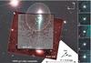 |
Fig. 1 SDSS gri colour composite mosaic of the IKN dSph field and its five known GCs. These are indicated with squares in the colour image and shown magnified on the right from the HST/ACS image data. The labels indicate the field of view for the archival HST/ACS F606W,F814W and our WHT/LIRIS KS-band image. The light-colour stellar density contour map is adapted from Fig. 6 in Lianou et al. (2010). The ellipse indicates the HyperLEDA values for the IKN diameter (2.69′ = 2.91 kpc) and ellipticity (0.18). For reference, with the arrows we indicate the direction to the group dominant galaxies M 81 and M 82. |
2.2. Data reduction and photometry
2.2.1. LIRIS data reduction
The NIR imaging reduction was performed within the LIRIS IRAF package LIRISDR2. For each night the data was first corrected for the pixel mapping anomaly with the lcpixmap IRAF task, an effect produced by the reconstruction of the two-dimensional array that misplaces some of the pixels, especially in the lower left quadrant.
The images were flat-field-corrected and sky-subtracted using the ldedither LIRISDR task for each night. One of the first corrections was the flat-fielding, which must correct not only for large scale gradients in the image but also for pixel-to-pixel gain variations. The dome flat fields were obtained by subtracting dark frames from bright frames of the same exposure time in order to suppress the possible thermal contamination of the telescope environment and then coadded and normalized for each night. The sky-subtraction step is the most important step in the data reduction of NIR data because the brightness and structure of the NIR sky varies on a timescale of minutes, and its contribution must be individually subtracted for each pixel. The general idea is to obtain the median frame for a set of images, discarding the values of the pixels that have received flux from celestial objects, and then to subtract the median frame from the science frames. The ldedither procedure creates sky frames from sets of five consecutive (dithered) exposures and generates a sky-subtracted image for each frame before coaddition.
We aligned all non-registered, but sky-subtracted output images from ldedither using a custom IRAF procedure based on geomap, geotran, and imcombine IRAF tasks. We used a sigma-clipping coaddition algorithm, with a statistics region used to estimate the images’ zero offsets, and the images are scaled by their exposure time. Figure 1 shows the final overlap region of the LIRIS coadded image with the HST and SDSS DR10 data. The standard stars data were reduced using the same IRAF and LIRISDR procedures as for the IKN images. The more photometric night was March 16, to which all images were subsequently aligned and registered. The total exposure time in the final coadded image is 5505 s.
2.2.2. Ks-band photometry of IKN globular clusters
Aperture magnitudes of the clusters and of standard and field stars were measured with tasks in the IRAF DAOPHOT package. We did a curve-of-growth analysis with r = 2,3,4,...,40 pixel aperture radius for the GCs and high S/N, isolated field stars in the images, subsequently choosing a photometry radius of 12 pixels. This is about three times the average full width half maximum of stars and unresolved sources in the final co-added image. The curve-of-growth analysis from isolated stars allowed us to derive an aperture correction of 0.04 mag. PSF photometry was not possible because of how few good PSF stars there were to build a reliable PSF model.
The photometry is calibrated assuming a transformation equation of the form below, where the coefficients are derived from a least squares fit to the magnitudes of the photometric standards:  (1)where KS and ks are the standard and instrumental magnitudes, pk = −0.07 ± 0.02 is the atmospheric extinction coefficient (Chies-Santos et al. 2011b), xkeff the effective airmass, and V the V-band magnitude of the standard stars adopted from Jenkner et al. (1990). Because of the low number of K-band standards with reliable published V-band magnitudes, the value of the colour term c was adopted to be 0.02, as found in earlier studies (Goudfrooij et al. 2001; Georgiev et al. 2012). The zero point was evaluated from the fit to the standard stars to be 23.01 ± 0.02 mag, which is not too different from the value found by (Chies-Santos et al. 2011b) of 23.07 ± 0.01 mag for another set of observations.
The final calibrated KS-band magnitudes of the clusters were estimated by using their V-band magnitude published in Georgiev et al. (2009b), iterating Eq. (1)until the KS magnitude converged. The V and KS magnitudes were also corrected for foreground galactic extinction with values for the total absorption of AV = 0.22 mag, AKs = 0.02 mag taken based on Schlafly & Finkbeiner (2011) recalibration of the Schlegel et al. (1998) dust maps assuming the Fitzpatrick (1999) reddening law with RV = 3.1.
The foreground reddening-corrected IKN GCs photometry is tabulated in Table 4.
2.2.3. Search for GC candidates in SDSS DR10
Since HST/ACS field of view covers half of IKN, we utilize the wide spatial and spectral coverage of SDSS to search for GC candidates. IKN dSph is not entirely covered by the HST/ACS field of view, and the stellar density map (Lianou et al. 2010) indicates that the centre of the IKN field stars is approximately at the location of the bright foreground star near the edge of the field of view (see Fig. 1, also Sect. 3.4). Therefore, given the apparent distribution of GCs on one side of IKN additional GCs may be located outside the HST/ACS image. Searching for GC candidates beyond the optical extent of IKN is also motivated by the discovery of very distant GCs around the dwarf irregular galaxy NGC 6822 located out to 11 kpc from the galaxy centre (Hwang et al. 2011). These GCs have similar luminosities, sizes and spatial distributions as the known IKN GCs (see Sects. 4 and 3.5).
To search for GC candidates in IKN, we make use of their nature as extended objects. HST/ACS derived half-light radii for the known GCs are in the range 1.96 ± 0.16 pc to 14.81 ± 0.83 pc (Georgiev et al. 2009b). The r-band seeing of the SDSS images used is 1.55′′, which corresponds to a projected spatial scale at the IKN distance of 27 pc. This implies that at least the larger half-light radii GCs will have a PSF that differs from a point-source PSF.
Although the model and PSF magnitudes in the SDSS photometric catalogues are quite reliable, we performed our own PSF photometry on archival SDSS images to evaluate the difference between stellar PSF and GC profiles and search for new cluster candidates. The additional reason for doing our own PSF analysis is that IKN falls on two SDSS stripes, which requires a separate PSF analysis. We find the difference between the PSFs of the two stripes to be well within the measurement uncertainty. We selected isolated, high S/N stars to build a PSF model and performed PSF photometry on all detected objects with the IRAF’s DAOPHOT package procedures (psf and alltstar). Instrumental PSF magnitudes were calibrated to standard SDSS magnitudes by using the SDSS PSF magnitudes of the same stars. The final SDSS photometry of the IKN GCs is tabulated in Table 4.
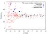 |
Fig. 2 Selection of GC candidates based on sharpness value. Shown is a g-band example of the sharpness value versus magnitude for all sources with PSF photometry (small crosses), the known IKN GCs (large solid, blue circles), and the SDSS GC candidates (open circles). The PSF stars are shown with small solid symbols (dark circles). |
Because the clusters were not detected or had S/N that was too low in the u-band images, this band was not used in the subsequent analysis. We used the sharpness value returned by allstar during the PSF fitting to search for objects more extended than the stellar PSF with a similar sharp value to the known GCs. The allstar sharpness parameter is defined as the difference between the squares of the width of the PSF model and the width of the object. That is, sources with light profile similar to the stellar PSF will have sharpness value close to 0, while more extended sources will have a sharpness value greater than 0. The extended nature of the candidates can be seen in Fig. 2, where the sharpness values for PSF stars, GCs and all other objects are plotted as a function of their g-band magnitude. The second selection criteria was based on colours, with the candidates having to be in the immediate vicinity of the GC’s in the griz colour space (within 2σ from the average GC colours).
One of the new GC candidates is very close to the bright foreground star (BD69+557), which prevents reliable photometry. Therefore we do not consider it for further analysis.
3. Analysis and discussion
3.1. GCs’ colours, photometric age, mass, and metallicity
To gain insight into the formation epochs of the IKN GCs and the evolutionary path of this faint dSph, we discuss the stellar population age and metallicity of the IKN GCs based on their optical-NIR integrated colour distributions. As mentioned earlier, we take advantage of the good age and metallicity resolution provided by the optical-NIR colour−colour indices.
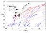 |
Fig. 3 Foreground reddening-corrected optical - NIR colour−colour plot, vs. of the IKN globular clusters (solid labelled circles). The cluster colours are compared to Bruzual & Charlot (2003) SSP model isometallicity tracks (M/H labelled lines) and isochrones (age-labelled lines). The top left arrows show the direction of increasing age and metallicity and the arrow to the right shows a reddening vector of AV = 0.5 mag. |
Figure 3 shows the (V − I)0 vs. (I − Ks)0 colour−colour distribution of all GCs in the IKN dSph, compared to Bruzual & Charlot (2003) SSP models for a canonical (Kroupa 2001) IMF and a range in age and metallicity as indicated by the labels. The distribution of the GCs’ colours in Fig. 3 suggests that all of them are likely old and metal-poor [ M / H ] ≤ −0.7 dex. This is consistent with the metal-poor and old age inferred for the brightest IKN GC-5 from recent spectroscopic analysis (Larsen et al. 2014a). However, given the photometric uncertainties, ages as young as 2−5 Gyr cannot be ruled out. In general, although with lesser certainty, the photometric metallicity spread of the IKN GCs is consistent with that of the IKN field stars, [ Fe / H ] ≤ −1.0 dex (Lianou et al. 2010).
To derive photometric ages and metallicities for the GCs in our sample we performed a minimization interpolation between the age and metallicity in the Bruzual & Charlot (2003) SSP model grid. These are estimated with the average value between the two closest values weighted by the distance to the respective model and the photometric uncertainty. This method enables us to derive upper and lower errors for the photometric ages and metallicities. The validity of this approach has been discussed in detail for the M 31 and MW GC colours with Bruzual & Charlot (2003) SSP tracks for old ages (e.g. Puzia et al. 2002; Georgiev et al. 2012). The GCs that fall outside of the model grid have age and metallicity derived from the nearest age and metallicity model tracks. A comparison of this technique for different SSP model tracks is presented in Georgiev et al. (2012). Errors due to the choice of the SSP model are included in our measured values and amount to about 10% at given age and metallicity. Thanks to the combination of optical-NIR magnitudes, uncertainty in derived cluster mass due to stochastic effects are below the 1−5% level for old and massive GCs, ≳ 105 M⊙ (Fouesneau & Lançon 2010; Fouesneau et al. 2012). In Table 2 the measured values for the photometric age, metallicity, and mass of the IKN GCs are tabulated.
To convert from colour-magnitude to metallicity-mass distributions, we used the SSP model M/LV values based on the GC’s colours to convert from luminosities to masses (for the adopted distance to IKN, see Sect. 1). The resulting mass-metallicity distribution is shown in Fig. 4. The absolute values for the metallicities of the IKN GCs range from −1.6 dex to −1.1 dex, are relatively metal-poor, and are also consistent with metallicity values of the IKN foreground stars (Lianou et al. 2010). Figure 4 shows that the photometric GC ages are older than about 10 Gyr and have a narrow spread. This suggests that the early formation of all clusters occurred within a relatively short time scale, which is typically the case for the old GCs in other galaxies, such as in the Milky Way or the old GCs in the LMC (see more detailed discussion of IKN RGB and GCs’ metallicity distributions in Sect. 3.3).
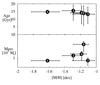 |
Fig. 4 Mass-metallicity (top) and age-metallicity (bottom) distributions of the IKN GCs (solid labelled circles) derived from their VIK magnitudes. |
Photometric metallicity, age, and mass of IKN GCs.
3.2. IKN peak SFR from its most massive GC
It has been demonstrated that there is an observational relation between the galaxy SFR and the luminosity of its most massive cluster at a given epoch (Larsen & Richtler 2000; Weidner et al. 2004; Maschberger & Kroupa 2007; Bastian 2008). Here we derive the IKN peak SFR from the photometric mass of the IKN most massive GC identically to Georgiev et al. (2012). Briefly, this included a correction for GC mass loss due to stellar evolution using the Bruzual & Charlot (2003) SSP M/LV ratios at 10 Myr. We have not accounted for mass loss from tidal shocking, which however, could be expected to be small for such a low mass dwarf. Because the suggested age spread among the IKN GCs is very small (cf. Fig. 4), the IKN peak SFR is calculated from its most massive cluster. For reference, we show in Fig. 5 the age against the SFR derived for each GC. It is clear that the peak star formation of at least 10 M⊙/year in IKN occurred around 14 Gyr ago. The most massive GC provides a lower limit of the SFR at  Gyr (the errors are propagated from the GCs mass uncertainties). The duration of the star formation burst cannot be estimated with high precision without good knowledge the GCs ages. However, given the low mass of the IKN and assuming a constant SFR, we can constrain the maximum length of the burst to a only a few (ten) million years. This indicates that IKN went through a bursty star formation episode at the epoch of the GCs formation.
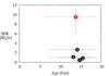 |
Fig. 5 Star formation rate calculated for each IKN GC against cluster age. The most massive GC (GC-5) yields a SFR of 10 M⊙/year at the time of GCs formation. |
The very small number of GCs means that one must keep in mind that statistical effects in the GC mass distribution might play a significant role in the SFR that we find for IKN.
The new GC candidates are either outside the HST and WHT field of view or within the region rendered unusable for analysis by the bright star. Thus, the candidates could not be confirmed visually on the HST image and that the NIR data is not available for breaking the age-metallicity degeneracy.
Moreover, we also compared the IKN GCs with the GC systems of the luminous elliptical galaxies M87 and M60 from Chies-Santos et al. (2011a). IKN GCs 4 and 5 fall on the same loci as M87/M60 GCs in the gzk parameter space, while the others do not have gzk photometry.
3.3. Metallicity distributions of GCs and field RGB stars − implications for IKN SFH
The comparison between the metallicity distributions of the GCs and IKN’s field stellar population and using the knowledge of the galaxy SFR, can provide important insight about how much of the initial star formation took place in star clusters. To be able to directly compare the metallicity distribution function (MDFs) of the IKN GCs with that of the RGB field stars we convert their total metal content ([M/H], derived in Sect. 3.1 from SSP models) into [Fe/H]. For that we use the Salaris et al. (1993) relation between [M/H] and [Fe/H] (their Eq. (3)), where the factor fα = 10α with α = 0.3 dex, accounts for the typical high α-element abundance (i.e. low Fe content) observed in GCs (cf. Eq. (1) in Ferraro et al. 1999). The converted [M/H] to [Fe/H] metallicity values for the IKN GCs are given in Table 2.
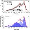 |
Fig. 6 Top: metallicity distribution of IKN field RGB stars (solid, red-line histogram) and IKN GCs (labelled solid circles). For viewing purposes, the vertical position of the GCs is scaled according to their mass. Thick solid (black) and dashed (grey) curves are the scaled probability density estimate (ρ⋆,RGB) and its 1σ estimated from the model PDFs (thin grey lines, details in Sect. 3.3). Bottom: mixture model of the IKN field RGB stars metallicity distribution. The best-fit maximum-likelihood mixture model probability density distribution is shown with the solid blue curve and its components by filled-curve Gaussians. For comparison we show again the metallicity distribution of IKN field RGB stars (solid red-line histogram). The percent fraction of each fitted Gaussian is given in the legend and Table 3. |
Figure 6 shows the direct comparison between the MDFs of RGB field stars and IKN GCs. For viewing purposes only, the y-axis values of the GCs are obtained by multiplying their photometric mass, ℳGC, (cf Table 2) by 1.5 × 10-4. Lianou et al. kindly provided us with the photometry of the IKN field RGB stars, which MDF is shown Fig. 6. Lianou et al. (2010) have already reported that IKN has a broad MDF which peaks at higher [Fe/H] than for such low-luminosity dwarf galaxy. This suggests that IKN has likely experienced a complex SFH with probably more than one burst of star formation.
To assess the significance and the likelihood of a multimodal, as opposed to a unimodal, MDF and compare the fraction of stars in GCs, we performed a more detailed statistical analysis with packages in R3. First, we estimated the [Fe/H] probability density function (PDF) of the RGB stars using an Epanechnikov kernel density estimator. We used this PDF as a prior and the [Fe/H] uncertainty of the RGBs to generate a large number of models (1000). The different model realizations are shown in Fig. 6. The joint PDF of all the models, as a function of [Fe/H], gave the final PDF of the RGB stars [Fe/H] distribution. We show this and its corresponding one sigma intervals in Fig. 6. This test confirms that there is a dip in the IKN field RGB’s MDF at the 1σ level.
To test the significance of the 1σ dip in the IKN MDF further, we performed an additional mixture-model statistical analysis to test whether the MDF is consistent with one or multiple underlying distributions. This particular test will allow us to assess whether the observed MDF can be represented by the combination of more than one Gaussian distribution. This will allow the fraction of the stellar population that falls into the same metallicity range as the old GCs to be derived, i.e. within the same SF epoch. For that we used routines in the mixdist and mixtools R packages with which we fit a mixture Gaussian distribution models to the data by the method of maximum likelihood minimization. We performed a mixture models with one, two, three, four, five, and six Gaussian components. The four Gaussian model was the preferred solution with the best statistics by far (smallest χ2 and highest p value) of all models. Models with more Gaussians give a marginally better χ2, but at the same time give the worst p value. This is because all components are simultaneously fit and likelihoods maximized. We can thus conclude from our statistical test that more than one component is needed to reproduce the MDF of the IKN RGB stars. We also note that only the four component model gave a good representation of the metal-poor peak at [ Fe / H ] ≃ −2.2 dex. It is beyond the scope of this paper to investigate further exactly how many components, i.e. episodes of star formation, could have been responsible for the present-day IKN field RGB’s MDF. The values for each of the four fitted components are given in Table 3.
Coefficients of the different Gaussian mixture model components.
Our mixture model fitting suggests that nearly a third (about 28%) of the IKN field stars are in the most metal-rich component, while the remaining 72% of the metal poorer RGB stars could have formed in more than one SF event. The uncertainties in the parameters of the three metal-poor components (see values in Table 3) prevent us from a firmer and more detailed discussion of whether and how many episodes of SF IKN could have went through. In addition, whether a Gaussian or another function would be a better description is also beyond the scope of this paper. For the following discussion we consider that up to 72% of the IKN star formation occurred simultaneously with the epoch at which the GCs formed. This stems from the distribution of the IKN GCs in Fig. 6a) compared to the field stellar component of IKN, which falls in the metal-poorer component.
We can first calculate the fraction of mass in clusters to total galaxy stellar mass. Summing up cluster masses in Table 2 gives ℳGC,tot = 8.14 × 10⁵ M⊙. For a total IKN luminosity of MV = −11.2 mag and M/LV = 3 for [ Fe / H ] = −1.0 dex and an age of 12 Gyr, the IKN mass is thus ℳ⋆,IKN = 7.7 × 10⁶ M⊙. Therefore we obtain a mass fraction of fℳ,GC = 0.106; i.e., 10.6% of the IKN stellar mass is in its old GCs. This is unusually high compared to the fraction of light or mass in GCs in more massive early- and late-type galaxies (e.g. Peng et al. 2008; Georgiev et al. 2010; Harris et al. 2013). If we consider our results from the mixture models above, i.e. that probably about 72% of the stars in IKN have formed in the same star formation episode as the old GCs, we will arrive at an even greater fraction of about 14%.
It is interesting to ask how the fraction fℳ,GC relates to the actual number of stars that formed in clusters, Γ = CFR / SFR, introduced by Bastian (2008). We can use the SFR = 10 M⊙/yr value obtained in Sect. 3.2 and calculate the surface SFR, ΣSFR. We adopt a radius equal to the optical extent of IKN, r = 1.5 kpc. Thus, ΣSFR = 1.4 M⊙/yr/kpc. This value for ΣSFR suggests that Γ should be in the range Γ = 10−30% based on the Γ − ΣSFR relation recently investigated for a wide range of environments (e.g. Bastian 2008; Goddard et al. 2010; Kruijssen 2012; Mora et al. 2014). This further confirms that IKN had a very intense SFH that lead to high CFRs and to the very high present-day number of old GCs.
3.4. Spatial distributions of the IKN GCs
Investigating whether the mass of the IKN GCs varies as a function of the galactocentric distance may hold important information about cluster formation and migration due to dynamical friction. Here we attempt to derive a new centre of IKN from the stellar positions of its RGB stars.
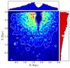 |
Fig. 7 Two-dimensional number density and histogram projection distributions of the IKN field stars. The histograms have a bin width of 0.345 kpc and are fitted with a Gaussian function shown with solid lines. The outer countour line in the 2D plot indicates a stellar number density of 17.5 ⋆/arcsec2 (16 ⋆/pc2). The white star indicates our best fit position of the IKN centre with an uncertainty of ±150 pc. |
Deriving the radial distribution of the GCs from the IKN centre is a rather complicated task because of the partial coverage of the HST/ACS field and the strong incompleteness due to the bright foreground star. To derive the photometric centre of IKN, we used the positions of the field stars detected in the HST/ACS image whose photometric and spatial data was provided to us by Lianou et al. (2010, priv. comm.). In Fig. 7 we show the 2D number density distribution of the IKN field stars. To minimize the impact of the foreground star on deriving the IKN photometric centre, our approach is first to obtain the histogram distributions along the x- and y-axes of the ACS field and then to fit a Gaussian functions to each. Their peaks positions are adopted as the IKN photometric centre. The IKN photometric centre derived using this method is shown in Fig. 7 with coordinates of RA = 10:08:05.8 and Dec = + 68:25:20 and with a total uncertainty of 8.5′′ (150 pc) derived from the fit. We note that the probably the choice of a Gaussian function may not be optimal, but given all other involved uncertainties, it is sufficient for our analysis. Additionally, to obtain a more realistic constraint to the IKN centre we fitted ellipses to the arcs defined by the constant surface stellar density contours. The 2D surface density of the RGB stars was estimated in a running window with a width of 300 pixels (15′′). The fit was performed for the arcs that are 300 pixels inwards from the ACS detector edges and with constant surface density between 3 and 6 stars/arcsec2. The results is that the centre is at RA = 10:08:24 ± 45″; Dec = + 6:24:47 ± 73″, PA = 154.4 ± 11.1 degrees (position angle east of north), ellipticity = 0.216 ± 0.12 (ϵ = 1 − b/a).
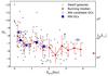 |
Fig. 8 Globular cluster luminosity versus projected distance form galaxy photometric centre for GCs in dwarf galaxies (small grey circles), IKN known GCs (large blue squares), and IKN GC candidates (large open squares). The running median (red diamonds) is computed from the entire dwarf galaxies GC sample with a bin size of 0.345 Kpc, where the y error bar is the standard deviation of the number of GCs in each bin. |
We can use the centre of IKN to see how the GCs are distributed as a function of the projected galactocentric distance. The radial distribution of the IKN GCs is shown in Fig. 8, where we also show the projected radial distributions of GCs from a larger sample of dwarf galaxies from Georgiev et al. (2008, 2009b). In general, Fig. 8 shows that the cluster luminosity (mass) decreases with increasing galactocentric distance. The high-mass clusters are closer to the centre. To quantify this trend for the combined Rproj distributions from all dwarf galaxies, we calculated the running median as a function of Rproj with a bin size of 0.345 kpc. Here we confirm an earlier finding that more luminous clusters in dwarf galaxies are typically more centrally located (Georgiev et al. 2009a). Clearly, Fig. 8 shows that the most massive IKN GC is closest to the derived here photometric centre. A likely explanation is that dynamical friction may have “sorted” the IKN GCs. However, spectroscopic observations are required to know the local velocity field and whether dynamical friction can be an efficient process for IKN central stellar density.
3.5. Alignment of IKN GCs and orientation in the M 81 group
We also report that the IKN GCs projected positions appear to be linearly aligned. Although this could be also a chance alignment due to low number statistics, the exact spatial and kinematic structure of the IKN GCs needs to be spectroscopically confirmed, because it can have important implications for interpreting the formation origin of IKN, its SFH and interaction within the M 81 group of galaxies. Furthermore, a similar linear alignment has been previously reported for the old GCs in NGC 6822 (Hwang et al. 2011; Huxor et al. 2013).
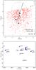 |
Fig. 9 Top: spatial distribution of the IKN GCs (large solid circles). The fitted linear regression through their position is shown with solid line, while the IKN major axis and orientation are shown with dashed and light gray line and ellipse, respectively. IKN RGB stars are shown with small (red) dots. Bottom: positions of galaxies associated to the M 81 group according to Karachentsev et al. (2002). Circle sizes are proportional to the galaxy absolute B-band luminosity. The line passing through IKN roughly shows the orientation of its GCs from the top panel. |
The projected linear alignment between the IKN GCs can already be seen in Fig. 1. In Fig. 9a) we show the straight-line, least squares fit through the GCs’ positions. For reference, we show with an ellipse the size of IKN’s Holmberg diameter, 2.69 kpc, (measured at μB = 25 mag) and its ellipticity, ϵ = 1 − b/a = 0.18, retrieved from the HyperLEDA and NED databases. For the centre of the ellipse we used the centre we obtained in Sect. 3.4. We note, however, that the relative uncertainty in the IKN ellipticity and particularly in the orientation of its major axis reaches nearly 100%. This thus prevents us from a more reliable discussion on the alignment between the IKN’s major axis and the fitted line through the positions of its GCs.
In the bottom panel of Fig. 9 we compare the orientation of the GCs alignment plane with respect the large scale distribution of galaxies within the M 81 group. If the GC alignment is due to their formation in a disk or triggered by interactions with galaxies in the M 81 group, angular momentum conservation arguments would suggest a correlation with the positions of the nearest galaxies and the larger structure in the group. Figure 9 shows that the GC’s projected alignment and the IKN’s major axis seem to be orthogonal to the larger scale galaxy distribution, i.e. the plane connecting IC 2547−NGC 3077−M 81. However, spectroscopic observations are required in order to properly describe the kinematics of the IKN GCs, whether they are indeed on a (rotating?) disk and what the orientation is of the vector of the angular momentum.
3.6. Implications for the formation origin of IKN
The unusual and probably complex star formation history of IKN were the first hints of the presence of a large number of old GCs compared to its total luminosity, i.e. the highest known GC specific frequency of SN = 126 (Georgiev et al. 2009b, 2010). Subsequently, resolved stellar population HST/ACS CMD analysis (Lianou et al. 2010) revealed that IKN has a very broad metallicity distribution function. It peaks at much higher metallicity for the IKN luminosity, unlike other early-type dwarf galaxies in the M 81 group with similar luminosity (Lianou et al. 2010). This led those authors to consider IKN as a galaxy that may have formed as a tidal dwarf galaxy during galaxy-galaxy interactions in the M 81 group. Recently, Larsen et al. (2014a) have performed a direct spectroscopic comparison between the brightest IKN GC-5 and those of another faint dwarf galaxy − WLM. It shows that in both galaxies the GCs are metal poor, although the IKN-05 GC spectra has a very low S/N.
Our analysis here further strengthens the idea of a complex SFH for IKN, based on its GCs’ ages, metallicity, and spatial distributions. Although the photometric uncertainties lead to large errors in these quantities, the photometric ages and metallicities of the GCs place them amongst the metal poor field stellar component (cf. Fig. 6). This suggests that the GCs and the metal-poor field stellar component have formed during the same burst of star formation. Our analysis of the field RGB star MDF suggests that there must have been at least two major star formation episodes in the IKN SFH. If galaxy-galaxy interactions in the M 81 group have triggered bursts of intense star formation, likely galactic pericentre passages were responsible for the multiple-peaked SFH. If IKN has formed as a tidal dwarf galaxy, one would also expect that it has a higher metallicity for its luminosity, which is the case. The apparent alignment of the IKN GCs, if real, also suggests that IKN could be a dSph transformed from a late-type disk dwarf.
The relevant observational evidence for a complex SFH of IKN are: i) on average slightly more metal-rich GCs [ Fe / H ] = −1.4 dex (cf. Fig. 6) than is typical for a truly metal-poor GC population of [ Fe / H ] ≪ −1.7 dex, e.g. in the Fornax dSph all GCs are with [ Fe / H ] < −2.0 dex (Larsen et al. 2014b; Hendricks et al. 2014); ii) non-unimodal MDF of the field RGB stars combined with the apparent alignment of the IKN GCs place constraints to the possible scenarios that could have led to the complex IKN SFH. Namely, 1) the IKN GCs should have formed together with the main galaxy stellar population, so that the GC and the RGB metallicities and MDFs are matched (Fig. 6); 2) this must have happened more than 5−8 Gyr ago; 3) the intensity of star formation must be such that it leads to the formation of an unusually large number of GCs; or 4) IKN must have lost at least 50% of its initial mass for it to lead to the high GC specific frequency. Tidal formation origin and/or the tidal-interaction-triggered star formation scenarios can match these observations. However, if IKN is a primordial dwarf it must contain a significant amount of dark matter, which cannot be estimated for the currently available data. Clearly, a spectroscopic follow up is needed to assess the dynamics of the system.
4. Summary and conclusions
We have presented a new K-band photometric analysis of the GCs of the IKN dwarf spheroidal using data taken with the NIR detector (LIRIS) installed on the 4.2 m William Herschel Telescope. Combined with existing HST/ACS V and I data, we effectively resolved the age-metallicity degeneracy in the I − Ks vs. V − I colour space. The new KS-band photometry is presented in Table 4.
-
Using SDSS DR10 archival images, we performed a PSF photometric analysis to look for GC candidates in the field around IKN that is not covered by the HST/ACS observations. We found two new GC candidates based on departure from a stellar PSF (cf. Fig. 2, Sect. 2.2.3). One of the candidates (GC-6) is, however, very close to a bright star, which renders its measured parameters highly inaccurate. High spatial and spectral resolution and multi-wavelength observations are required to reveal the nature of these two objects. If one of these GC candidates proves to be another genuine GC, this will make IKN the galaxy that formed GCs with a very high efficiency per unit luminosity with one of the highest specific frequencies known to date, SN = 126.
-
To derive GCs’ photometric ages, masses, and metallicities for all known GCs in the IKN galaxy in Sect. 3.1, we interpolated between Bruzual & Charlot (2003) SSP model tracks (cf. Fig. 3). For all GCs we derived a mean photometric age that is consistent with the oldest ages in the SSP model grid (
Gyr, Fig. 4, Table 2). The old GC age indicates an ancient burst of star formation. Using the empirically established observational relation between the most massive cluster and the galaxy SFR (see Sect. 3.2), we found that the burst of star formation led to the formation of 3 × 10⁵ M⊙ GC was about 10 M⊙/year about 14 Gyr ago (cf. Fig. 5, in Sect. 3.2). Table 4Photometric properties of the IKN globular clusters (GCs) and the new candidates (GCCs).
-
We derived GC metallicities in the range 2.0 < [ Fe / H ] < −1.2 dex (Table 2, Sect. 3.3). These are consistent with the metal-poor component of the metallicity distribution function of the field RGB stellar population of IKN reported by Lianou et al. (2010). Our reanalysis of the field RGB stars MDF, data kindly provided to us by Lianou et al., confirms their finding of a broad MDF. However, we found at least two major bursts of star formation with small statistical significance, the most recent of which produced the most metal-rich stellar population with a peak of [ Fe / H ] ≃ −1.0 dex (Fig. 6). Although the photometric metallicities of the IKN GCs are large, they are more consistent with the metal-poor component. Our mixture model analysis suggests that about 72% of the IKN stellar population could have formed at the same star-formation epoch as the bulk of the IKN GCs. We note, however, that a spectroscopic confirmation is needed to firmly establish the IKN metallicities. For GC-5 such a confirmation does exist, though, and falls at the lower end of the error interval of the photometric estimate.
-
We found that the more luminous (massive) IKN GCs are usually distributed towards the centre of IKN (Sect. 3.4), which is consistent with earlier observations (cf. Fig. 8). It has been suggested that such mass segregation arises from dynamical friction,which is efficient in low-velocity systems, but strongly depends on the local stellar density. Further spectroscopic observations are required to map the velocity field of IKN and establish whether dynamical friction would be efficient for such a low stellar surface density galaxy.
-
We find that the projected positions of the IKN GCs appear to be aligned. (Fig. 9, Sect. 3.5). This is similar to the observed alignment of the GCs in the Local Group dSph NGC 6822 (Hwang et al. 2011; Huxor et al. 2013). It remains to be shown spectroscopically whether the IKN GCs have disk kinematics or the apparent distribution is a chance alignment. Knowing this will help for interpreting the IKN origin, since a merger of dwarf galaxies will destroy existing disk structures (Bekki 2008). The orientation of the plane of alignment of the IKN GCs appears to be very close to the orientation of the IKN major axis, but the latter is very poorly constrained. Looking at the orientation of the GC alignment compared to the large scale distribution of galaxies tentatively reveals that it is orthogonal to the large plane that connects several of the M 81 group galaxies (see Sect. 3.5 and Fig. 9 bottom panel).
In summary, the large cluster formation efficiency for each galaxy mass, high GC metallicities, and positional alignment, point towards a complex SFH for IKN. Whether the tidal origin scenario for the galaxy indeed holds remains to be confirmed through further spectroscopic investigations.
Package written by Jose Acosta Pulido to manage data produced by the LIRIS instrument −www.iac.es/galeria/jap/lirisdr/LIRIS_DATA_REDUCTION.html
R is a free software environment for statistical computing. http://www.r-project.org/
Acknowledgments
A.T. is supported by the DFG Emmy Noether grant Hi 1495/2-1 and the Bonn-Cologne Graduate School of Physics and Astronomy. I.G. would like to thank the science department and “International Research Fellow” programme of ESA-ESTEC in Noordwijk for the partial support during the completion of this paper. A.C.S. acknowledges the receipt of CNPq/BJT-A fellowship 400857/2014-6. The authors would like to thank Sophia Lianou for kindly providing us with their photometic tables and measurements of the IKN field RGB stars metallicities. We are also grateful for the helpful discussions with Søren Larsen and the anonymous referee. This research made use of the NASA/IPAC Extragalactic Database (NED), which is operated by the Jet Propulsion Laboratory, California Institute of Technology, under contract with the National Aeronautics and Space Administration. We acknowledge the use of the HyperLeda database (http://leda.univ-lyon1.fr).
References
- Abazajian, K. N., Adelman-McCarthy, J. K., Agüeros, M. A., et al. 2009, ApJS, 182, 543 [NASA ADS] [CrossRef] [Google Scholar]
- Ashman, K. M., & Zepf, S. E. 1992, ApJ, 384, 50 [NASA ADS] [CrossRef] [Google Scholar]
- Bastian, N. 2008, MNRAS, 390, 759 [NASA ADS] [CrossRef] [Google Scholar]
- Bekki, K. 2008, MNRAS, 388, L10 [Google Scholar]
- Bridges, T. J., Hanes, D. A., & Harris, W. E. 1991, AJ, 101, 469 [NASA ADS] [CrossRef] [Google Scholar]
- Brodie, J. P., & Strader, J. 2006, ARA&A, 44, 193 [NASA ADS] [CrossRef] [Google Scholar]
- Brodie, J. P., Romanowsky, A. J., Strader, J., et al. 2014, AJ, 796, 52 [CrossRef] [Google Scholar]
- Bruzual, G., & Charlot, S. 2003, MNRAS, 344, 1000 [NASA ADS] [CrossRef] [Google Scholar]
- Cantiello, M., & Blakeslee, J. P. 2007, ApJ, 669, 982 [NASA ADS] [CrossRef] [Google Scholar]
- Chies-Santos, A. L., Larsen, S. S., Kuntschner, H., et al. 2011a, A&A, 525, A20 [NASA ADS] [CrossRef] [EDP Sciences] [Google Scholar]
- Chies-Santos, A. L., Larsen, S. S., Wehner, E. M., et al. 2011b, A&A, 525, A19 [NASA ADS] [CrossRef] [EDP Sciences] [Google Scholar]
- Chies-Santos, A. L., Larsen, S. S., Cantiello, M., et al. 2012, A&A, 539, A54 [NASA ADS] [CrossRef] [EDP Sciences] [Google Scholar]
- Croxall, K. V., van Zee, L., Lee, H., et al. 2009, ApJ, 705, 723 [NASA ADS] [CrossRef] [Google Scholar]
- Dalcanton, J. J., Williams, B. F., Seth, A. C., et al. 2009, ApJS, 183, 67 [NASA ADS] [CrossRef] [Google Scholar]
- Ferraro, F. R., Messineo, M., Fusi Pecci, F., et al. 1999, AJ, 118, 1738 [NASA ADS] [CrossRef] [Google Scholar]
- Fitzpatrick, E. L. 1999, PASP, 111, 63 [NASA ADS] [CrossRef] [Google Scholar]
- Forbes, D. A., Brodie, J. P., & Grillmair, C. J. 1997, AJ, 113, 1652 [NASA ADS] [CrossRef] [Google Scholar]
- Fouesneau, M., & Lançon, A. 2010, A&A, 521, A22 [NASA ADS] [CrossRef] [EDP Sciences] [Google Scholar]
- Fouesneau, M., Lançon, A., Chandar, R., & Whitmore, B. C. 2012, ApJ, 750, 60 [NASA ADS] [CrossRef] [Google Scholar]
- Georgiev, I. Y., Goudfrooij, P., Puzia, T. H., & Hilker, M. 2008, AJ, 135, 1858 [NASA ADS] [CrossRef] [Google Scholar]
- Georgiev, I. Y., Hilker, M., Puzia, T. H., Goudfrooij, P., & Baumgardt, H. 2009a, MNRAS, 396, 1075 [NASA ADS] [CrossRef] [Google Scholar]
- Georgiev, I. Y., Puzia, T. H., Hilker, M., & Goudfrooij, P. 2009b, MNRAS, 392, 879 [NASA ADS] [CrossRef] [MathSciNet] [Google Scholar]
- Georgiev, I. Y., Puzia, T. H., Goudfrooij, P., & Hilker, M. 2010, MNRAS, 406, 1967 [NASA ADS] [Google Scholar]
- Georgiev, I. Y., Goudfrooij, P., & Puzia, T. H. 2012, MNRAS, 420, 1317 [NASA ADS] [CrossRef] [Google Scholar]
- Goddard, Q. E., Bastian, N., & Kennicutt, R. C. 2010, MNRAS, 405, 857 [NASA ADS] [Google Scholar]
- Goudfrooij, P., Alonso, M. V., Maraston, C., & Minniti, D. 2001, MNRAS, 328, 237 [NASA ADS] [CrossRef] [Google Scholar]
- Hargis, J. R., & Rhode, K. L. 2012, AJ, 144, 164 [NASA ADS] [CrossRef] [Google Scholar]
- Harris, W. E. 1991, ARA&A, 29, 543 [NASA ADS] [CrossRef] [Google Scholar]
- Harris, W. E. 2010, Roy. Soc. London Phil. Trans. Ser. A, 368, 889 [Google Scholar]
- Harris, W. E., & van den Bergh, S. 1981, AJ, 86, 1627 [NASA ADS] [CrossRef] [Google Scholar]
- Harris, W. E., Kavelaars, J. J., Hanes, D. A., Pritchet, C. J., & Baum, W. A. 2009, AJ, 137, 3314 [NASA ADS] [CrossRef] [Google Scholar]
- Harris, W. E., Harris, G. L. H., & Alessi, M. 2013, ApJ, 772, 82 [NASA ADS] [CrossRef] [Google Scholar]
- Hempel, M., Kissler-Patig, M., Hilker, M., et al. 2003, in Extragalactic Globular Cluster Systems, ed. M. Kissler-Patig, 125 [Google Scholar]
- Hempel, M., Zepf, S., Kundu, A., Geisler, D., & Maccarone, T. J. 2007, ApJ, 661, 768 [NASA ADS] [CrossRef] [Google Scholar]
- Hendricks, B., Koch, A., Walker, M., et al. 2014, A&A, 572, A82 [NASA ADS] [CrossRef] [EDP Sciences] [Google Scholar]
- Huxor, A. P., Ferguson, A. M. N., Veljanoski, J., Mackey, A. D., & Tanvir, N. R. 2013, MNRAS, 429, 1039 [NASA ADS] [CrossRef] [Google Scholar]
- Hwang, N., Lee, M. G., Lee, J. C., et al. 2011, ApJ, 738, 58 [NASA ADS] [CrossRef] [Google Scholar]
- Jenkner, H., Lasker, B. M., Sturch, C. R., et al. 1990, AJ, 99, 2082 [Google Scholar]
- Karachentsev, I. D., Dolphin, A. E., Geisler, D., et al. 2002, A&A, 383, 125 [NASA ADS] [CrossRef] [EDP Sciences] [Google Scholar]
- Karachentsev, I. D., Tully, R. B., Dolphin, A., et al. 2007, AJ, 133, 504 [NASA ADS] [CrossRef] [Google Scholar]
- Kissler-Patig, M. 2000, in Extragalatic Globular Cluster Systems: A new Perspective on Galaxy Formation and Evolution, ed. R. E. Schielicke, Rev. Mod. Astron., 13 [Google Scholar]
- Kroupa, P. 2001, MNRAS, 322, 231 [NASA ADS] [CrossRef] [Google Scholar]
- Kruijssen, J. M. D. 2012, MNRAS, 426, 3008 [NASA ADS] [CrossRef] [Google Scholar]
- Lada, C. J., & Lada, E. A. 2003, ARA&A, 41, 57 [NASA ADS] [CrossRef] [Google Scholar]
- Larsen, S. S., & Richtler, T. 2000, A&A, 354, 836 [NASA ADS] [Google Scholar]
- Larsen, S. S., Brodie, J. P., Forbes, D. A., & Strader, J. 2014a, A&A, 565, A98 [NASA ADS] [CrossRef] [EDP Sciences] [Google Scholar]
- Larsen, S. S., Brodie, J. P., Grundahl, F., & Strader, J. 2014b, ApJ, 797, 15 [NASA ADS] [CrossRef] [Google Scholar]
- Lianou, S., Grebel, E. K., & Koch, A. 2010, A&A, 521, A43 [NASA ADS] [CrossRef] [EDP Sciences] [Google Scholar]
- Maschberger, T., & Kroupa, P. 2007, MNRAS, 379, 34 [NASA ADS] [CrossRef] [Google Scholar]
- Mora, M. D., Chanamé, J., & Puzia, T. H. 2014, AJ, submitted [arXiv:1411.7314] [Google Scholar]
- Muratov, A. L., & Gnedin, O. Y. 2010, ApJ, 718, 1266 [NASA ADS] [CrossRef] [Google Scholar]
- Peng, E. W., Jordán, A., Côté, P., et al. 2008, ApJ, 681, 197 [NASA ADS] [CrossRef] [Google Scholar]
- Peng, E. W., Ferguson, H. C., Goudfrooij, P., et al. 2011, ApJ, 730, 23 [NASA ADS] [CrossRef] [Google Scholar]
- Puzia, T. H., Zepf, S. E., Kissler-Patig, M., et al. 2002, A&A, 391, 453 [NASA ADS] [CrossRef] [EDP Sciences] [Google Scholar]
- Salaris, M., Chieffi, A., & Straniero, O. 1993, ApJ, 414, 580 [NASA ADS] [CrossRef] [Google Scholar]
- Schlafly, E. F., & Finkbeiner, D. P. 2011, ApJ, 737, 103 [NASA ADS] [CrossRef] [Google Scholar]
- Schlegel, D. J., Finkbeiner, D. P., & Davis, M. 1998, ApJ, 500, 525 [NASA ADS] [CrossRef] [Google Scholar]
- Tonini, C. 2013, ApJ, 762, 39 [NASA ADS] [CrossRef] [Google Scholar]
- Villegas, D., Kissler-Patig, M., Jordán, A., Goudfrooij, P., & Zwaan, M. 2008, AJ, 135, 467 [NASA ADS] [CrossRef] [Google Scholar]
- Weidner, C., Kroupa, P., & Larsen, S. S. 2004, MNRAS, 350, 1503 [NASA ADS] [CrossRef] [Google Scholar]
- Worthey, G., Faber, S. M., Gonzalez, J. J., & Burstein, D. 1994, ApJS, 94, 687 [NASA ADS] [CrossRef] [Google Scholar]
All Tables
Photometric properties of the IKN globular clusters (GCs) and the new candidates (GCCs).
All Figures
|
Fig. 1 SDSS gri colour composite mosaic of the IKN dSph field and its five known GCs. These are indicated with squares in the colour image and shown magnified on the right from the HST/ACS image data. The labels indicate the field of view for the archival HST/ACS F606W,F814W and our WHT/LIRIS KS-band image. The light-colour stellar density contour map is adapted from Fig. 6 in Lianou et al. (2010). The ellipse indicates the HyperLEDA values for the IKN diameter (2.69′ = 2.91 kpc) and ellipticity (0.18). For reference, with the arrows we indicate the direction to the group dominant galaxies M 81 and M 82. |
| In the text | |
|
Fig. 2 Selection of GC candidates based on sharpness value. Shown is a g-band example of the sharpness value versus magnitude for all sources with PSF photometry (small crosses), the known IKN GCs (large solid, blue circles), and the SDSS GC candidates (open circles). The PSF stars are shown with small solid symbols (dark circles). |
| In the text | |
|
Fig. 3 Foreground reddening-corrected optical - NIR colour−colour plot, vs. of the IKN globular clusters (solid labelled circles). The cluster colours are compared to Bruzual & Charlot (2003) SSP model isometallicity tracks (M/H labelled lines) and isochrones (age-labelled lines). The top left arrows show the direction of increasing age and metallicity and the arrow to the right shows a reddening vector of AV = 0.5 mag. |
| In the text | |
|
Fig. 4 Mass-metallicity (top) and age-metallicity (bottom) distributions of the IKN GCs (solid labelled circles) derived from their VIK magnitudes. |
| In the text | |
|
Fig. 5 Star formation rate calculated for each IKN GC against cluster age. The most massive GC (GC-5) yields a SFR of 10 M⊙/year at the time of GCs formation. |
| In the text | |
|
Fig. 6 Top: metallicity distribution of IKN field RGB stars (solid, red-line histogram) and IKN GCs (labelled solid circles). For viewing purposes, the vertical position of the GCs is scaled according to their mass. Thick solid (black) and dashed (grey) curves are the scaled probability density estimate (ρ⋆,RGB) and its 1σ estimated from the model PDFs (thin grey lines, details in Sect. 3.3). Bottom: mixture model of the IKN field RGB stars metallicity distribution. The best-fit maximum-likelihood mixture model probability density distribution is shown with the solid blue curve and its components by filled-curve Gaussians. For comparison we show again the metallicity distribution of IKN field RGB stars (solid red-line histogram). The percent fraction of each fitted Gaussian is given in the legend and Table 3. |
| In the text | |
|
Fig. 7 Two-dimensional number density and histogram projection distributions of the IKN field stars. The histograms have a bin width of 0.345 kpc and are fitted with a Gaussian function shown with solid lines. The outer countour line in the 2D plot indicates a stellar number density of 17.5 ⋆/arcsec2 (16 ⋆/pc2). The white star indicates our best fit position of the IKN centre with an uncertainty of ±150 pc. |
| In the text | |
|
Fig. 8 Globular cluster luminosity versus projected distance form galaxy photometric centre for GCs in dwarf galaxies (small grey circles), IKN known GCs (large blue squares), and IKN GC candidates (large open squares). The running median (red diamonds) is computed from the entire dwarf galaxies GC sample with a bin size of 0.345 Kpc, where the y error bar is the standard deviation of the number of GCs in each bin. |
| In the text | |
|
Fig. 9 Top: spatial distribution of the IKN GCs (large solid circles). The fitted linear regression through their position is shown with solid line, while the IKN major axis and orientation are shown with dashed and light gray line and ellipse, respectively. IKN RGB stars are shown with small (red) dots. Bottom: positions of galaxies associated to the M 81 group according to Karachentsev et al. (2002). Circle sizes are proportional to the galaxy absolute B-band luminosity. The line passing through IKN roughly shows the orientation of its GCs from the top panel. |
| In the text | |
Current usage metrics show cumulative count of Article Views (full-text article views including HTML views, PDF and ePub downloads, according to the available data) and Abstracts Views on Vision4Press platform.
Data correspond to usage on the plateform after 2015. The current usage metrics is available 48-96 hours after online publication and is updated daily on week days.
Initial download of the metrics may take a while.