| Issue |
A&A
Volume 581, September 2015
|
|
|---|---|---|
| Article Number | A59 | |
| Number of page(s) | 11 | |
| Section | Numerical methods and codes | |
| DOI | https://doi.org/10.1051/0004-6361/201423465 | |
| Published online | 02 September 2015 | |
A new approach to multifrequency synthesis in radio interferometry
1 Max-Planck Institut für Astrophysik, Karl-Schwarzschild-Str. 1, 85748 Garching, Germany
e-mail: This email address is being protected from spambots. You need JavaScript enabled to view it.
2 Ludwig-Maximilians-Universität München, Geschwister-Scholl-Platz 1, 80539 München, Germany
Received: 19 January 2014
Accepted: 18 February 2015
Abstract
We present a new approach to multifrequency synthesis in radio astronomy. Using Bayesian inference techniques, the new technique estimates the sky brightness and the spectral index simultaneously. In principle, the bandwidth of a wide-band observation can be fully exploited for sensitivity and resolution, currently only limited by higher order effects like spectral curvature. Employing this new approach, we further present a multifrequency extension to the imaging algorithm resolve. This method also delivers a reconstruction of the most probable spectral index spatial correlation structure across the source and an estimate of the spectral index uncertainty, although at a comparably high computational cost. In simulations, this new algorithm can outperform current multifrequency imaging techniques.
Key words: instrumentation: interferometers / methods: data analysis / methods: statistical / techniques: image processing / techniques: interferometric / radio continuum: general
© ESO, 2015
1. Introduction
In radio astronomy, multifrequency observations are widely used for many different purposes. Examples include the investigation of spectral line emission, analyzing continuous synchrotron spectra of radio sources, determination of Faraday rotation in polarization imaging, correlating brightness structures at largely different wavelengths, or improving the sensitivity and coverage of an interferometer without introducing more antennas into the array (for a review see, e.g., Taylor et al. 1999). Most of these tasks only become possible with observations that span over many frequencies and data analysis methods that can handle these kinds of observations.
For the remainder of this work, we focus entirely on multiwavelength radio continuum studies in total intensity. Neither spectral line observations, polarization imaging, nor wavelengths studies beyond pure radio observations will be a direct topic. In Sect. 4, we will comment on possible extensions of the presented work into other domains of multifrequency radio astronomy.
Historically in radio interferometry, the term “multifrequency synthesis” is mainly used to denote techniques that focus on the direct combination of single-instrument observations at different frequencies to improve the resolution and sensitivity of a radio interferometer (see Conway et al. 1990, and references therein). For this purpose, a number of methods have been devised, most notably double deconvolution (Conway et al. 1990) and multifrequency CLEAN (Sault & Wieringa 1994). These methods usually work by Taylor expanding a spectral model function around a reference frequency. We comment on these methods in more detail in Sect. 2.1.
Conversely, investigating the spectral behavior of a radio synchrotron source on its own usually is achieved through totally independent standard imaging of the surface brightness in the sky at a number of frequencies. Resolution is kept uniform over all frequencies to correctly recombine the images at individual frequencies. Subsequently, the spectral parameters are determined by fitting a function through all the single frequency images, usually assuming a power-law shaped spectral evolution.
Only recently, implementations of MF-CLEAN also make it possible to constrain the spectral properties (see Rau & Cornwell 2011), effectively starting to merge both multifrequency high-resolution imaging and spectral analysis into one algorithm. This combined notion, allows us to interpret and use the term multifrequency synthesis.
Further development of multifrequency imaging techniques is paramount for being able to fully exploit the data from the new generation of radio telescopes, such as the upgraded VLA, LOFAR, the SKA pathfinder missions or ultimately the SKA itself (see, e.g., Garrett 2012). Their unprecedented broadband frequency coverages of many GHz of possible bandwidths and previously unknown frequency regimes offer many advances in astrophysical and cosmological sciences. At the same time, however, they raise a challenge for current data analysis methods (see Sect. 2.1). One aspect of this challenge arises from the fact that current algorithms might not meet the expected sensitivity or fidelity because previously acceptable models and approximations break down with the quality and quantity of data now available. The other aspect is that the huge quantities encompassed in new data sets represent an extreme computational challenge on their own, regardless of the algorithms used. It should be emphasized that this study focuses entirely on the first aspect of the challenge (for this topic, see also Sect. 4).
We present a new approach that uses Bayesian statistical inference techniques to combine a simultaneous statistical estimation of the sky brightness and the spectral behavior with the benefits in resolution and sensitivity of classical multifrequency synthesis. Conceptually, this new approach has a number of advantages over standard methods. In principle, the full bandwidth of the observation is used for maximum theoretical sensitivity. No subsequent imaging at all single frequencies is employed and, thereby, fewer reconstruction artifacts are introduced and no artificial downgrading of resolution is necessary. Our model for the spectral behavior is not approximated through Taylor expansions around a frequency, and at the moment only is limited by possible higher order effects like spectral curvature. In this way, our approach is conceptually very similar to the new method of Faraday synthesis (Bell & Enßlin 2012) in polarization imaging (see Sect. 2.2 for more details). Furthermore, the spatial correlation of the parameters describing the spectral behavior is used to constrain and improve the estimation of spectral properties, and can further be viewed as a new scientific result on its own. Finally, it is possible to approximate the statistical uncertainty of the spectral index estimate in addition to that of the total intensity.
To demonstrate the viability of our new approach, we present a multifrequency extension to the radio extended emission imager resolve (Junklewitz et al. 20159) as an alternative to multiscale, multifrequency CLEAN (Rau & Cornwell 2011), the standard method for wide-band multifrequency synthesis of extended radio sources.
For our derivations, we often refer to the work presented in Junklewitz et al. (20159), henceforth Res2013.
2. Theory and algorithm
In this section, we first briefly review the current status of multifrequency synthesis techniques (Sect. 2.1), then develop the new approach (Sect. 2.2) based on information field theory (Enßlin et al. 2009) and the inference framework presented in Res2013. We further present a multifrequency extension to the imaging algorithm resolve (see Res2013) using the developed framework (Sect. 2.2).
2.1. Multifrequency aperture synthesis and spectral index reconstruction
Aperture synthesis is the technique of connecting an array of telescopes in such a way that we can effectively synthesize a combined instrument with a much larger aperture and therefore resolution (Ryle & Hewish 1960; Thompson et al. 1986). It can be shown that for observations at a single frequency ν0, and under the assumption of measuring the sky as flat in a plane tangent to the phase center of the observation, this kind of radio interferometer approximately takes incomplete samples of the Fourier transformed brightness distribution in the sky (Thompson et al. 1986),  (1)For our purposes, working under this assumption suffices for the analysis we undertake. For a detailed derivation of (1) consider Thompson et al. (1986). The quantity V(u,v) is called the visibility function. The coordinates u and v are vector components describing the distance between a pair of antennas in an interferometric array, where this distance is usually referred to as a baseline. They are given in numbers of wavelengths, with u and v usually parallel to geographic east-west and north-south, respectively. The coordinates l and m are a measure of the angular distance from the phase center along axes parallel to u and v, respectively. The function W(u,v) defines the sampling given by the layout of the interferometric array. This function is zero throughout most of the u,v-space, apart from where measurements have been made where it is taken to be unity.
The visibility function is what our instrument measures, but we are actually interested in the brightness distribution of the source in the sky. Unfortunately, an inversion of (1) does not give us the true brightness distribution, but its convolution with the inverse Fourier transform of the sampling function, better known as the ”dirty beam” Idb = ℱ-1W:  (2)Here, we have introduced a symbolic Fourier operator ℱkx = exp( − i(ul + vm)) with x = (l,m) and k = (u,v), the common notation ID, named “dirty image”, for the simple Fourier inversion of the visibilities, and the symbol ∗ to denote a convolution operation.
For imaging at a single frequency, one usually proceeds using a deconvolution algorithm aiming to solve (2) approximately. The most common algorithm is CLEAN (Högbom 1974), or one of its many variants (Clark 1980; Schwab 1984; Sault & Wieringa 1994; Cornwell 2008; Rau & Cornwell 2011). These algorithms basically model the sky brightness to be a collection of delta peak point sources or more complex, size-varying basis functions like Gaussians, which are iteratively assigned by searching for the peak values in the dirty image. Alternatives exist, however, especially for imaging extended emission, like the maximum entropy method (Cornwell & Evans 1985), adaptive scale pixel decomposition (Bhatnagar & Cornwell 2004) or the recently published Bayesian extended emission imager resolve (Res2013), which we use in an expanded multifrequency version (see Sects. 2.2 and 3).
Originally, radio telescopes observed with relatively narrow bandwidths and at only a few different frequencies. The standard approach for imaging the spectral properties of a source since then is to take single frequency observations, or observations averaged over close channels for higher sensitivity, image them separately, and then fit a spectral model to the observations. Since continuous synchrotron emission is known to show a power-law spectrum (Rybicki & Lightman 1985), for many astrophysical purposes the following model is sufficient:  (3)Sometimes, higher order spectral deviations are modeled with a second term in the exponential of (3),
  (4)effectively enhancing the linear function in log I vs. log ν space (3) to a quadratic polynomial. This model is referred to as spectral curvature.
Simultaneous multifrequency imaging at different frequencies has been introduced to radio astronomy upon the realization that observations at many frequencies, if stacked together appropriately, can improve the sampling in the uv-plane (see Conway et al. 1990, and references therein). This way, the sensitivity of a radio interferometric observation can be enhanced considerably. Because the uv-coordinates are measured in numbers of wavelengths, the same interferometer samples different parts of the Fourier space at different frequencies. An interferometer includes N(N − 1)/2 baselines and therefore uv points, where N is the number of antennas. In theory, observing at a number of frequencies Nf enhances the measured baselines to NfN(N − 1)/2, which is the equivalent effect of introducing roughly  extra antennas (Conway et al. 1990).
This approach was first developed by Conway et al. (1990) for midsized fractional bandwidths of around ± 10%, together with the method of double deconvolution to mitigate spectral errors when using CLEAN for a spectrally combined data set. Later, double deconvolution was developed into the more advanced multifrequency CLEAN (MF-CLEAN; Sault & Wieringa 1994) and multifrequency multiscale CLEAN (MF-MS-CLEAN; Rau & Cornwell 2011).
All these methods assume the spectral dependence to be a power law, like Eqs. (3) or (4) and propose to approximate this spectral function during the CLEAN-like deconvolution process with a Taylor expansion. To our knowledge, current implementations use a few terms of a Taylor expansion in ν or log ν around a reference frequency ν0. Rau & Cornwell (2011) argue that a direct decomposition into one or two terms of a polynomial in log I vs. log ν would actually be the most accurate representation1, but for current implementations this is discarded by them because of numerical instabilities.
During the CLEAN deconvolution process, the iteratively updated sky model is used to also update the coefficients of the spectral Taylor expansion. With this method, spectral index or even spectral curvature can be constrained by these coefficients. Care must be taken, since this expansion is usually stopped after a few terms and might not be valid over large bandwidths.
For modern wide-band data sets from the new generation of instruments, spanning several GHz of bandwidths, this means that probably even more emphasis must be put onto the handling of the spectral effects, either by invoking higher order terms in the expansions (see Sault & Wieringa 1994; Rau & Cornwell 2011) or by exploring a different approach. In principle it would be desirable to statistically infer the full structure of I(l,m,ν) directly from the data using a global optimization function without explicit modeling of the spectral dependence. A similar approach was actually mentioned by Conway et al. (1990), but found to be unnecessarily complicated and computationally expensive for the typically modest fractional bandwidths at the time.
For similar reasons of feasibility, we now consider an approach that still explicitly models the frequency dependence, but uses prior knowledge to derive a statistically optimal solution in the sense of Bayesian reasoning.
2.2. A multifrequency extension to the algorithm RESOLVE
We often refer to the detailed derivations layed out in Sect. 2 and Appendix 1 of Res2013 that form the basis from which we derive our multifrequency algorithm.
We start by summarizing (1) and (3) into a multifrequency measurement model, i.e.,  (5)where again x = (l,m) and k = (u,v), the term n(k,ν) introduces measurement noise, the data d(k,ν) has been introduced, which is basically the visibility function with measurement noise, and the spectral dependence of the source I(x,ν) is kept general for the moment.
To simplify notation and identify (5) as a general inverse inference problem as analyzed in Res2013, we henceforth drop all explicit dependence on k and x and combine all known instrumental effects into a response function Rν: = W(k,ν)ℱ, leading to  (6)There are many instrumental effects beyond the sampling in the uv-plane given by W(k,ν) such as an antenna sensitivity pattern or a direction dependent, variable sampling. Nevertheless, we keep the basic definition Rν: = W(k,ν)ℱ and refer to Res2013 concerning the possibility of including other effects within this framework. We just emphasize that, without loss of generality, most of these effects can be in principle included2. We also assume the instrument to be fully calibrated, and thus the response Rν to be known.
In accordance with standard radio interferometric literature (Thompson et al. 1986), we assume Gaussian noise statistics, mainly induced by the antenna electronics and independent of measurements at different frequencies and time steps of the observation (Thompson et al. 1986). Henceforth, the noise nν will be assumed to be drawn from a multivariate, zero mean Gaussian distribution of dimension nd, i.e.,  (7)Solving (6) exactly for Iν is not possible, since all information is lost on the Fourier modes not sampled by Rν. This is just a different way of stating that a direct Fourier inversion of (1) yields the dirty image and not an exact representation of the sky brightness.
Instead, the aim is to find a statistical estimate for the most probable sky brightness signal in a full Bayesian sense, given all observational and noise constraints. In Res2013, it was shown in detail how this can be done in a Bayesian statistical framework for a radio astronomical data model like (1). We briefly repeat the main points, and otherwise refer to Res2013.
To find an optimal statistical estimate for the sky brightness signal Iν, we regard it as a random field with certain a priori statistical properties expressed in the prior distribution P(I), but fully constrained by the data through the statistics of the likelihood distribution P(d | I). The likelihood distribution summarizes how the data are obtained with a measurement of the true sky brightness signal, and for our problem can be expressed as  (8)which is a Gaussian over dν − RνIν with the covariance structure of the uncorrelated noise
  .
.
Prior and likelihood statistics can be combined into the posterior distribution P(I | d) ∝ P(d | I)P(I), which holds the important information of how much the sky brightness signal is statistically constrained by the data. From there, an estimate for the signal can be obtained by calculating a suitable statistic of the posterior, most prominently its mean or its mode, corresponding to the minimization of different error norm measures between the signal and its estimate (see Res2013; or Jaynes 2003; Caticha 2008 and Lemm 1999; Enßlin et al. 2009, for a comprehensive review of Bayesian reasoning or inference on fields).
The exact choice of an appropriate inference algorithm at this stage largely depends on the complexity of the problem (i.e., the posterior). For the problem at hand, since the likelihood is already known (8), this comes down to the question of the prior statistics of Iν.
The most general way conceivable would be to not explicitly model the spectral dependence of I(x,ν) at all, as for instance in (3) or (4). Instead, I(x,ν) can be interpreted as a three-dimensional continuous field and should be inferred as a whole from the entire data. In general, let us assume not only point-like but also extended emission in the sky, and some kind of extended structure in spectral space as well. In such a setting, I(x,ν) could be set a priori as a statistical field with an unknown and probably nonisotropic cross-correlation structure in the combined sky and spectral space. This complex, unknown cross-correlation structure, on the one hand complicates the problem enormously, but, on the other hand, could be used to guide the reconstruction, if correctly estimated with the field itself.
A number of statistical methods have already been developed to handle simpler problems of signal reconstructions with unknown but isotropic correlation structure, many of them solving the problem for Gaussian fields using information field theory (Enßlin & Frommert 2011; Enßlin & Weig 2010) or Gibbs sampling Monte Carlo methods (Sutter et al. 2012; Karakci et al. 2013), or recently also for lognormal fields (Enßlin & Frommert 2011; Enßlin & Weig 2010; Oppermann et al. 2013; Greiner 2013; Selig & Enßlin 2015). Most notably this method was also used to create resolve (Res2013). A full combined spatial and spectral reconstruction, as outlined above, would require substantial further development and is outside of the scope of this work.
We can choose a more direct strategy still residing within our approach of statistical inference, but fix a spectral model and infer instead the spectral index (or curvature) as a field on its own. In the following, we choose the model (3) for the simplicity of the approach and for a functional similarity with the algorithm resolve that makes it very natural to include in a combined method.
resolve works under the assumption that the extended surface brightness at a single frequency is a priori assumed as a random field drawn from log normal statistics (Res2013). For our multifrequency problem, this basically turns (6) into ![Mathematical equation: \begin{eqnarray} d_\nu &=& R_\nu I_\nu + n_\nu \notag\\ &=& R_\nu \left[I_{0}(l,m,\nu_0) \ \left(\frac{\nu}{\nu_0}\right)^{-\alpha}\right] + n_\nu \notag\\ &=& R_\nu \left[\rho_0 \ \mathrm{e}^{s(l,m)} \ \left(\frac{\nu}{\nu_0}\right)^{-\alpha}\right] + n_\nu, \label{resolve} \end{eqnarray}](/articles/aa/full_html/2015/09/aa23465-14/aa23465-14-eq50.png) (9)where s is a Gaussian random field (such that the logarithm of es is a Gaussian random field again), and ρ0 is a constant to normalize the system to the right units, for example. Although, the frequency dependence of s was not explicitly shown in Res2013, the derivation of resolve implicitly assumed the algorithm to work for a single frequency in the way presented here. resolve assumes the spatial correlation of an extended source in the sky to be reflected by the covariance of the Gaussian random field s, which is unknown a priori, and thus estimated from the data itself together with the sky brightness. The covariance S of a Gaussian field is equivalent to its two-point correlation function and is handled as such by resolve in form of the power spectrum , which is the Fourier transformation of the correlation function3. A deeper analysis of this can be found in Res2013.
(9)where s is a Gaussian random field (such that the logarithm of es is a Gaussian random field again), and ρ0 is a constant to normalize the system to the right units, for example. Although, the frequency dependence of s was not explicitly shown in Res2013, the derivation of resolve implicitly assumed the algorithm to work for a single frequency in the way presented here. resolve assumes the spatial correlation of an extended source in the sky to be reflected by the covariance of the Gaussian random field s, which is unknown a priori, and thus estimated from the data itself together with the sky brightness. The covariance S of a Gaussian field is equivalent to its two-point correlation function and is handled as such by resolve in form of the power spectrum , which is the Fourier transformation of the correlation function3. A deeper analysis of this can be found in Res2013.
We now make the central assumption that the spectral index α can be modeled a priori as a Gaussian random field with its own spatial correlation structure in the sky. At least for an extended source, we have every reason to assume that the spectral index should be a field with spatial extension itself. Observational constraints strongly imply that typical extended radio structures also show extended and smooth spectral index structures, for instance, radio halos and relics of galaxy clusters (Feretti et al. 2012), radio galaxy lobes (Kassim et al. 2005), or supernova remnants (Green 2001).
In Res2013, we argued extensively that a Gaussian random field would be the ideal choice for a signal prior of an extended field with a priori unknown correlation structure, as long as the field is not assumed to vary strongly on orders of magnitude and not necessarily needs to be positive definite. Both constraints apply very well to known spectral index maps, where variations usually do not reach even one order of magnitude, and nothing prevents the spectral index in principle to change the sign. For details of these arguments see Res2013, we now proceed under this assumption.
If we rewrite (3) only slightly, we find,  (10)which reveals that, if α has a Gaussian prior, (10) naturally turns into a model for a lognormal prior, only different in shape (and more complicated) from (9) because of the term −ln(ν/ν0).
We have not specified I0(l,m,ν0) yet. Thus, at this point, our inference approach to multifrequency synthesis is in principle compatible with any method that reconstructs and deconvolves the surface brightness I0(l,m,ν0) at a single reference frequency ν. At least as long as it seems consistent with the source of interest to assume that the spectral index is an extended and spatially correlated field. In an extreme case, like single, unresolved point sources, this method probably will not yield optimal results.
We choose to combine (9) and (10) into one single method, where we assume our double lognormal measurement model to be ![Mathematical equation: \begin{eqnarray} d_\nu = R_\nu \left[\rho_0 \ \mathrm{e}^{s(l,m) - \ln{\left(\nu/\nu_0\right)} \alpha(l,m)}\right] + n_\nu, \label{mfresolve} \end{eqnarray}](/articles/aa/full_html/2015/09/aa23465-14/aa23465-14-eq61.png) (11)with ρ0 again a constant, from now on set to one w.l.o.g., and the signal fields s and α having Gaussian prior distributions P(s) and P(α), i.e.,
(11)with ρ0 again a constant, from now on set to one w.l.o.g., and the signal fields s and α having Gaussian prior distributions P(s) and P(α), i.e.,  We now write down a posterior distribution for each signal field, while the other field (and its covariance) is assumed to be known, held constant, and regarded as part of two distinct versions of the response operator Rν, henceforth called
 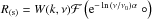 and
and 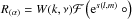 , where the symbol ° denotes where the field needs to be inserted that the operator acts on,
  As in Res2013, it is not possible to calculate the posterior mean for either of the two signal fields s or α without invoking complicated or expensive perturbation or sampling methods (see Res2013). We therefore continue to use the procedure already presented there, and calculate the posterior maximum to estimate both signals,
 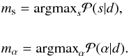 (16)In signal inference, this procedure is called maximum a posteriori (MAP; Jaynes 2003). The resulting fix-point equations from Eqs. (16) need to be solved numerically using a nonlinear optimization scheme. For this, we resort to the same implementations as in Res2013 (see Appendix 2 therein).
With this choice, we basically extend resolve to a multifrequency algorithm by integrating a second complete resolve step for the spectral index into the method, and iterating between the statistical estimation of s with its covariance S, and α with its covariance A. As outlined above, we always hold one of the fields (and their respective covariances) as constant and regard them as part of the response during this process.
It should be emphasized again that the resolve step for the spectral index could in principle be combined with any other method to reconstruct I0(l,m,ν0) at a single frequency ν0.
The exact equations that need to be solved to calculate (16) for either of the two fields and estimate their power spectra (i.e., their correlation structure in form of their Gaussian covariances, see above) are layed out in Appendix A and derived rigorously in Res2013.
3. Tests
We have integrated multifrequency capability into the existing implementation of resolve and tested the algorithm using simulated data4. The code is written in Python using the signal inference library NIFTy (Selig et al. 2013), for details of the implementation we refer to Appendix 2 of Res2013.
As in Res2013, we constructed simulated observations with the tool makems5 using a realistic uv-coverage from a Very Large Array (VLA) observation in its A-configuration. The VLA samples the uv-plane non uniformly at irregular intervals, and the response includes thereby a convolutional gridding and degridding operator using a Kaiser-Bessel kernel (for details see Appendix 2 in Res2013). We simulated observations over a range of 2 GHz at a reference frequency of 1.002 GHz, with 20 separate frequency channels. The observations are short snapshots of approximately 20 min per frequency, with a total of 42 120 visibility measurements at each frequency channel. This setting leads to an especially sparse sampling of the uv-plane at a single frequency, but to a much better coverage for the combined multifrequency data (for reference see Junklewitz et al. 20159).
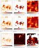 |
Fig. 1 Multifrequency reconstruction of the two signal fields es and α, observed with a sparse uv-coverage from a VLA-A-configuration. The images are 1002 pixels large, the pixel size corresponds to roughly 0.1 arcsec. The brightness units are in Jy/px. The ridge-like structures in the difference maps simply stem from taking the absolute value and mark zero-crossings between positive and negative errors. |
 |
Fig. 2 Comparison of different methods for spectral index reconstruction with differently strong masks. The images are 1002 pixels large, the pixel size corresponds to roughly 0.1 arcsec. First column: signal. Second column: resolve reconstruction. Third column: power-law fit. Fourth column: MS-MF-CLEAN. |
For all tests, the signal s is drawn from a Gaussian distribution, finally entering the formalism as an exact log normal field6.
To use a spectral index signal with some correlation to the brightness signal, we model the spatial source dependence of the spectral index in an ad hoc fashion.
For the spectral index signal α, we use a sum of two Gaussian fields (see Sect. 3.1), one being independently drawn, while the second is the surface brightness signal s itself, down-weighted with a suitable factor. The resulting spectral index signal varies smoothly between a (partly steep) declining spectrum (α = 0 − 1.22) mostly on the source, and flat to steeply rising spectra on the rest of the map (to α = 0 − ( − 3.66)). This is done to introduce a spectral index signal with some correlation to the surface brightness signal, at least in an ad-hoc fashion. Typically, extended sources in radio astrophysics show a spatial cross-correlation between both, which is a result of different physical processes underlying the structure and formation of these sources. A notable example are radio halos and relics in galaxy clusters (Feretti et al. 2012). Of course, our model is only an ad-hoc approximation of the proof of concept undertaken in this work. We also emphasize that such a cross-correlation between α and s is not exploited by resolve (see Sect. 2.2 for an outlook).
The complex, Gaussian input noise variance in uv-space is equal for all visibilities and frequencies. As with single-frequency resolve, the algorithm does not require equal noise variances and can in principle handle varying variances. The noise variance was set to a low7 value of σ2 = 10-3 Jy2.
In continuation with Res2013, we use a relative ℒ2 – norm measure of the difference in the signal to the reconstruction to measure the accuracy of the estimate of both brightness and spectral reconstructions, we find,  where the sums are taken over all pixels of the reconstruction. For the motivation behind this choice see Sect. 3 in Res2013.
In Sect. 3.1 we focus exclusively on the reconstruction of the two signals s and α. Then, in Sect. 3.2, we compare the results from multifrequency resolve with standard imaging procedures. The reconstruction of the signal power spectra is discussed separately in Sect. 3.3.
3.1. Main test results
We start by showing the reconstruction of the presented simulated observations using multifrequency resolve. In Fig. 1, a surface brightness and a spectral index signal are shown, together with the respective reconstructions obtained with resolve and absolute difference maps of both signals to their reconstructions. We show the spectral index maps in total and overlayed with a mask that focuses on the part of the observed field that contains the brightest part of the surface brightness signal. Later, in Fig. 2, we show the reconstruction for different masks (along with a comparison to other methods, see Sect. 3.2). We choose the three different masks mainly qualitatively by visual comparison to show only the parts of the sky with a surface brightness signal above a certain threshold. The actual threshold values for the surface brightness were 2 Jy/px, 4 Jy/px, and 6 Jy/px. These thresholds correspond to signal-to-noise ratios of 4.7, 10, and 14.4, calculated from the MSMF-Clean reconstruction8. In Fig. 1, the medium mask is displayed. The relative average error measures without masks are δI = 0.13 for the surface brightness, and δα = 0.34 for the spectral index (see Table 1 for a listing of all error measures for all masks).
It can be seen that resolve recovers the original surface brightness very accurately. For this particular choice of relative low noise, the algorithm succeeds in reconstructing even small scale features of the signal. The effects of the instrumental point spread function are successfully deconvolved. These findings are in perfect agreement with the results presented on single-frequency resolve in Res2013.
The general structure of the spectral index is well reconstructed, even for outer regions where the brightness signal is very weak and reaches the noise level or below. Over all, small scale features are much better recovered in the inner regions, where the main brightness sources are located, as can be seen by comparison between the full and the masked images in Fig. 1. It is expected that the quality of the spectral index reconstruction depends on the strength of the observed surface brightness, as is illustrated by the poor performance of the standard power-law fit in recovering any structures outside the strong source regions. This is presented in the next section (see Fig. 2). In most real applications, those regions with extremely low signal-to-noise in surface brightness usually are not in any focus of the investigation. We thus choose the relatively conservative mask in Fig. 1 to highlight this important part of the reconstruction. Nevertheless, it should be noted that, at least for this low noise example with relatively high sensitivity due to the broad bandwidth, resolve is able to reliably extrapolate its estimation into the weaker regions around the main sources also.
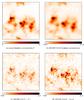 |
Fig. 3 Comparison of multifrequency resolve and MS-MF-CLEAN surface brightness reconstructions. The images are 1002 pixels large, and the pixel size corresponds to roughly 0.2 arcsec. The brightness units are in Jy/px. The ridge-like structures in the difference maps simply stem from taking the absolute value, marking zero-crossings between positive and negative errors. First row left: resolve reconstruction. First row right: MS-MF CLEAN reconstruction. Second row left: absolute per-pixel difference between the signal and the resolve reconstruction Second row right: absolute per-pixel difference between the signal and the MS-MF CLEAN reconstruction. |
In addition, with resolve, an uncertainty of the spectral index reconstruction can be estimated. As for the single frequency reconstructions presented in Res2013, the second derivative of the posterior is used to approximate its covariance Dα (for details, see Appendix A and Res2013). This way, the full estimate for the spectral index signal becomes  (19)For the given reconstruction, the relative uncertainty map is shown in the lower right of Fig. 1. Qualitatively, the map shows nicely that the reconstruction is most reliable where brightness is strong, and gives a consistent estimate over these regions. The regions of lowest brightness are not reliable in the present map and, are therefore masked in Fig. 1. As discussed in Res2013, the calculation of an uncertainty estimate is computationally costly. Because of the lack of accessible computer power for testing purposes, we stopped the calculations at a point likely before complete convergence and smoothed the outcome. Other than for low-brightness regions, this does not seem to be a principle problem, since the uncertainty is expected to be smooth and we are mainly interested in a proof of concept at this point. Because of this, and in general because of the nonlinear nature of the inference problem (16), the exact values of the uncertainty do not reflect a pure Gaussian covariance and effectively clearly underestimate the real error for this testing run.
3.2. Comparison to standard methods
In this section, we compare the results of multifrequency resolve with two standard methods: straight forward power law fit for (3) using single-frequency MS-CLEAN images, and an MF-MS-CLEAN reconstruction for the surface brightness and the spectral index. The reconstructions were performed on the same simulated observation as in Sect. 3.1. All results were obtained using the radio-astronomical software package CASA (Reid & CASA Team 2010). The MF-MS-CLEAN reconstructions were obtained using about 1500 iterations, a small gain factor of 0.2, uniform weighting and six different multiscales, ranging from a single pixel to moderately large structures. Two terms for the Taylor expansion in ν were used (see Sect. 2.1). In Fig. 2, a comparison is shown between resolve, a power-law fit, and MF-CLEAN results for the spectral index and differently strong masks. Only the brighter parts of the field are shown. In the masked, very low brightness regions, none of the algorithms (CLEAN, power law fit, resolve) could recover much structure due to a low signal-to-noise ratio. The resolve reconstruction of these regions shows relative uniform values close to the prior spectral index mean.
Error measures for these spectral index reconstructions are listed in Table 1. These show that resolve outperforms the other methods, in particular, in regions of lower brightness. In the brightest regions, the CLEAN algorithm performs comparably to resolve in terms of the error measure. However, there resolve has the significant advantage of providing a spectral index map that is better resolved spatially.
Figure 3 shows a comparison of multifrequency surface brightness reconstructions with resolve and MS-MF-CLEAN for the simulated observation of Sect. 3.1. For this simulation, resolve is more successful in reconstructing the overall structure, and especially recovers more of the small scales.
3.3. Power spectrum reconstructions
The power spectrum of the spectral index is reconstructed together with the field itself. It represents the spatial correlation of the spectral index over the observed sky. As explained in Sect. 2.2, we expect the typical spectral index structure of an extended (i.e., spatially correlated) radio source to be spatially correlated to itself. For all the details on power spectrum reconstructions, we refer to Res2013, since almost all derivations for standard single-frequency resolve power spectrum reconstructions are valid as well for the spectral index.
In this section we only discuss the spectral index power spectrum, since the reconstructions for the brightness power spectra are identical to those already presented in Res2013. We simply note that, in principle, a multifrequency reconstruction recovers structure on smaller scales, and thus, it is expected that multifrequency resolve should be able to map spatial power spectra up to higher Fourier modes (i.e., smaller correlation structures).
A typical result from multifrequency resolve is illustrated in Fig. 4. This figure shows the original spectral index power spectrum of the Gaussian signal field, used in the simulated observations of Sect. 3.1, and its reconstruction, which belongs to the same iteration step as the presented signal reconstructions earlier. The power spectrum is reconstructed relatively well, and no power is lost on high modes (i.e., small scales), which is just a consequence of the fact that the simulated observation was conducted with low noise.
As for the brightness reconstructions in Res2013, we emphasize that the power spectrum should not only be viewed as a by-product of the algorithm to accurately estimate the spectral index signal. For instance, some astronomical objects show very distinct spectral index structures and can even be classified after this criterion. A prominent example might be radio halos and relics of galaxy clusters, both of which typically show steep spectral indices that evolve spatially roughly like the source itself (Feretti et al. 2012). Measuring the spatial power spectra of these objects might lead to a more exact and quantitative classification scheme. Another application might lie in the investigation of different physical processes within a single source that lead to spectrally very different regions. Estimating the spectral correlation structure over these regions offers a new method of quantitative analysis of the interplay of these processes.
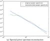 |
Fig. 4 Power spectrum reconstruction of the spectral index α for the reconstruction shown in Sect. 3.1 using multifrequency resolve and plotted against the corresponding spatial Fourier modes of the image. |
4. Conclusion
We presented a multifrequency extension to the imaging algorithm resolve (Junklewitz et al. 20159). The combined algorithm is optimal for multifrequency imaging of extended radio sources. It simultaneously estimates the surface brightness at a reference frequency and the spectral index of the source. Within the assumption of a spectral index model, no approximations or further parameter-dependent modeling is used in the spectral index reconstruction. Multifrequency resolve is thus capable of exploiting the full bandwidth of a modern radio observation for maximum sensitivity and resolution, and is only limited by higher order spectral effects like spectral curvature. In principle, an extension of this approach is conceivable that would use a spectral model-free, three-dimensional statistical field I(x,ν) that is reconstructed using a full spatial-spectral cross-correlation, but we leave this for future work.
Multifrequency resolve has been tested successfully using simulated observations of the VLA in its A-configuration. For the presented tests, the algorithm can outperform standard imaging methods in both surface brightness and spectral index estimations.
The algorithm uses a Gaussian prior and an effective log normal model for the spectral index. This approach is not necessarily restricted to a combination with single-frequency resolve, and can in principle be combined with any other imaging or deconvolution method for the surface brightness reconstruction.
For the sake of feasibility, many details of radio interferometric observations have been left out of the analysis. The response might realistically contain a number of additional effects, for instance an instrumental primary beam or wide-field and direction dependent effects. We refer to Junklewitz et al. (20159), where many of these problems already have been discussed.
In its current form, the presented algorithm has relatively high computational costs and numerical demands (for an analysis of algorithmic efficiency, see Junklewitz et al. 20159). In general, this is often true for many Bayesian statistical inference algorithms that use large covariance matrices or statistical sampling. This poses an obstacle for day-to-day applicability and basically prohibits use in online imaging, since modern broadband data sets especially tend to be very large, and therefore are already numerically challenging on their own. Since this study was centered on fundamental algorithmic development, numerical efficiency was not a focus. Future work is needed to obtain a more efficient implementation of the algorithm. Particular promising routes would be to exploit the computing power of GPUs or to integrate resolve into the very powerful standard radio imaging framework of major and minor cycles.
For the future, it seems to be desirable to refrain completely from an explicit spectral model, and try to infer a full, non parametric, three-dimensional spectral intensity I(l,m,ν). Possibly, this kind of development could benefit greatly from reconstructing a full cross-correlation structure between the sky and spectral space. We leave this more complete approach for a future publication.
Actually, for the spectral model (4), this would not be an approximation at all since it simply is a quadratic polynomial in log I vs. log ν space.
In principle this approach can be extended into a full RIME (radio interferometer measurement equation), considering all Stokes parameters and instrumental gains (Smirnov 2011a,b).
We actually assume the spatial correlation to be a priori rotationally and translationally invariant, and thus the power spectrum to be diagonal S(k,k′) = ⟨s(k)s(k′)†⟩ = (2π)nsδ(k − k′)Ps( | k |). However, this does not imply that the correlation structure must be invariant under any transformation a posteriori as well. A more detailed discussion can be found in Res2013.
To get access to the preliminary code prior to its envisaged public release, please contact This email address is being protected from spambots. You need JavaScript enabled to view it. or This email address is being protected from spambots. You need JavaScript enabled to view it.
In Res2013 it was demonstrated that resolve also works beyond that on realistic signals drawn from real CLEAN maps.
In comparison to the signal strength in Fourier space, the chosen value ensures a high signal-to-noise ratio. The unit Jy was used here for convenience. Effectively, it stands for whatever units the simulated signal is interpreted to be given in.
The signal-to-noise values are given for easier comparison to standard methods and thus are calculated using the CLEAN reconstruction. A similar, albeit less obvious, estimate can be given using the reconstructed uncertainty, for details see Junklewitz et al. (2015 9).
As a reminder: in (A.1) we use an implicit convention to sum or taking the integral over repeated discrete or continuous indices, see Res2013 for details.
This actually renders R(α) a nonlinear operator.
Acknowledgments
The authors like to thank Urvashi Rau for great help in obtaining high quality reconstructions with MSMF CLEAN.
References
- Bell, M. R., & Enßlin, T. A. 2012, A&A, 540, A80 [NASA ADS] [CrossRef] [EDP Sciences] [Google Scholar]
- Bhatnagar, S., & Cornwell, T. J. 2004, A&A, 426, 747 [NASA ADS] [CrossRef] [EDP Sciences] [Google Scholar]
- Caticha, A. 2008, ArXiv e-prints [arXiv:0808.0012] [Google Scholar]
- Clark, B. G. 1980, A&A, 89, 377 [NASA ADS] [Google Scholar]
- Conway, J. E., Cornwell, T. J., & Wilkinson, P. N. 1990, MNRAS, 246, 490 [NASA ADS] [Google Scholar]
- Cornwell, T. J. 2008, IEEE J. Select. Topics Signal Process., 2, 793 [Google Scholar]
- Cornwell, T. J., & Evans, K. F. 1985, A&A, 143, 77 [NASA ADS] [Google Scholar]
- Enßlin, T. A., & Frommert, M. 2011, Phys. Rev. D, 83, 105014 [NASA ADS] [CrossRef] [Google Scholar]
- Enßlin, T. A., & Weig, C. 2010, Phys. Rev. E, 82, 051112 [NASA ADS] [CrossRef] [Google Scholar]
- Enßlin, T. A., Frommert, M., & Kitaura, F. S. 2009, Phys. Rev. D, 80, 105005 [NASA ADS] [CrossRef] [Google Scholar]
- Feretti, L., Giovannini, G., Govoni, F., & Murgia, M. 2012, A&ARv, 20, 54 [Google Scholar]
- Garrett, M. A. 2012, in Proc. Meeting From Antikythera to the Square Kilometre Array: Lessons from the Ancients, PoS(Antikythera & SKA)041 [Google Scholar]
- Green, D. A. 2001, in AIP Conf. Ser. 558, eds. F. A. Aharonian, & H. J. Völk, 59 [Google Scholar]
- Greiner, M. 2013, Master Thesis, Ludwig-Maximilians-Universität München [Google Scholar]
- Högbom, J. A. 1974, A&AS, 15, 417 [NASA ADS] [Google Scholar]
- Jaynes, E. T. 2003, Probability Theory: The Logic of Science (CUP) [Google Scholar]
- Junklewitz, H., Bell, M. R., Selig, M., & Enßlin, T. A. 2015, A&A, in press, DOI: 10.1051/0004-6361/201323094 (Res2013) [Google Scholar]
- Karakci, A., Sutter, P. M., Zhang, L., et al. 2013, ApJS, 204, 10 [NASA ADS] [CrossRef] [Google Scholar]
- Kassim, N. E., Lazio, T. J. W., Lane, W. M., et al. 2005, in X-Ray and Radio Connections, eds. L. O. Sjouwerman, & K. K. Dyer [Google Scholar]
- Lemm, J. C. 1999, ArXiv e-prints [arXiv:physics/9912005] [Google Scholar]
- Oppermann, N., Selig, M., Bell, M. R., & Enßlin, T. A. 2013, Phys. Rev. E, 87, 032136 [NASA ADS] [CrossRef] [Google Scholar]
- Rau, U., & Cornwell, T. J. 2011, A&A, 532, A71 [NASA ADS] [CrossRef] [EDP Sciences] [Google Scholar]
- Reid, R. I., & CASA Team 2010, BAAS, 42, 568 [NASA ADS] [Google Scholar]
- Rybicki, G. B., & Lightman, A. P. 1985, Radiative processes in astrophysics (John Wiley & Sons) [Google Scholar]
- Ryle, M., & Hewish, A. 1960, MNRAS, 120, 220 [NASA ADS] [CrossRef] [Google Scholar]
- Sault, R. J., & Wieringa, M. H. 1994, A&AS, 108, 585 [NASA ADS] [Google Scholar]
- Schwab, F. R. 1984, AJ, 89, 1076 [NASA ADS] [CrossRef] [Google Scholar]
- Selig, M., & Enßlin, T. 2015, A&A, 574, A74 [NASA ADS] [CrossRef] [EDP Sciences] [Google Scholar]
- Selig, M., Bell, M. R., Junklewitz, H., et al. 2013, A&A, 554, A26 [NASA ADS] [CrossRef] [EDP Sciences] [Google Scholar]
- Smirnov, O. M. 2011a, A&A, 527, A106 [NASA ADS] [CrossRef] [EDP Sciences] [Google Scholar]
- Smirnov, O. M. 2011b, A&A, 527, A107 [NASA ADS] [CrossRef] [EDP Sciences] [Google Scholar]
- Sutter, P. M., Wandelt, B. D., & Malu, S. S. 2012, ApJS, 202, 9 [NASA ADS] [CrossRef] [Google Scholar]
- Taylor, G. B., Carilli, C. L., & Perley, R. A. 1999, in Synthesis Imaging in Radio Astronomy II, ASP Conf. Ser., 180 [Google Scholar]
- Thompson, A. R., Moran, J. M., & Swenson, G. W. 1986, Interferometry and synthesis in radio astronomy (New York: Wiley-Interscience) [Google Scholar]
Appendix A: Details of the algorithm
In this Appendix, we repeat some of the basic derivations from Res2013, and derive the details of how reconstructing the spectral index using resolve differs from the standard procedure presented there. In principle, many of the original derivations are still valid for multifrequency resolve, estimating s and α. The derivations for power spectrum reconstructions and uncertainty calculations remain especially close to the equations already presented in Res2013, and we do not repeat them explicitly here.
Appendix A.1: Reconstruction of the sky brightness signal field s
The estimation of the sky brightness at a reference frequency I0(l,m,ν0) = ρ0es(l,m) can mostly be conducted with the standard single-frequency resolve.
The only difference is the more complex response operator . Dropping the explicit signal index for a moment and writing the specific measurement model (11) for the signal s with explicit operator and field indices, 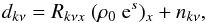 (A.1)reveals that the operator Rkνx actually spans the single-frequency Fourier transform over all observed frequencies into a large, many-frequency data space9. Conversely, the adjoint response now includes a sum over all frequencies to collapse everything back into the two-dimensional sky at reference frequency. Since both operations are used in resolve, it is by this procedure that the multifrequency resolve effectively uses uv-information at all frequencies to constrain the estimation of s. Of course, the quality of this reconstruction depends on the accuracy of the current estimation for α, used in the reconstruction step for s to define R(s).
Appendix A.2: Reconstruction of the spectral index α
The log normal model for the spectral index, e− ln(ν/ν0)α, only differs in the term b = − ln(ν/ν0) from the model used for the sky brightness signal. This slightly complicates the calculations for the signal estimation with MAP and the power spectrum reconstruction and eventual uncertainty calculation. For both, derivatives of the posterior (15) with respect to α are needed (see Res2013), and this will add extra b-terms into the equations. The results of this are summarized in Sect. A.3.
As for the sky brightness signal s (see Sect. A.1), the response operator for the α reconstructions R(α) = W(k,ν)ℱ(es(l,m) °) is more complex. Effectively, the b-term in the basic log normal model e− ln(ν/ν0)α would prevent us from just defining our signal space to be the two-dimensional sky since R(α) acts on e− ln(ν/ν0)α. In the actual implementation of the multifrequency resolve algorithm, we circumvent this problem by assuming that R(α) acts on α and all other terms, including the exponential operation of the log normal model, are part of the operator10. In this way, R(α) and can be understood to act in the same way as their respective counterparts for s do (i.e., they also span up and collapse into the full-frequency data space).
Appendix A.3: Combined algorithm
Using our findings in Res2013 and in the previous subsections, multifrequency resolve comes down to solving iteratively two only slightly different, subsequent sets of equations:
![Mathematical equation: \appendix \setcounter{section}{1} \begin{eqnarray} \notag\\[-10.5mm] &&p_i^s = \frac{\left(q_i^s + \frac{1}{2} \mathrm{tr} \left((m_{\mathrm{s}}{m_{\mathrm{s}}}^{\dagger} + D_{\mathrm{s}})S^{(i)}\right)\right)}{\left(\alpha_i^{(\mathrm{s-pr})} - 1 + \frac{\varrho_i}{2} + (Tp)_i\right)}\cdot \label{eq:three} \\ \notag\\ &&\mathrm{{\it Estimation \ of \ \alpha}} \notag\\ &&A^{-1}_{p} m_{\mathrm{\alpha}} + b \ \mathrm{e}^{b m_{\mathrm{\alpha}}} \cdot M_{\mathrm{\alpha}} \mathrm{e}^{b m_{\mathrm{\alpha}}} - j_{\mathrm{\alpha}} \cdot b \ \mathrm{e}^{b m_{\mathrm{\alpha}}} = 0 \label{eq:estimate_a one}\\ \notag\\[-1mm] &&\!\left(D_{\mathrm{\alpha}}\right)_{xy} = A^{-1}_{p \ xy} + b^2 \ \mathrm{e}^{b (m_{\mathrm{\alpha}})_x} \ (M_{\alpha})_{xy} \ \mathrm{e}^{b (m_{\mathrm{\alpha}})_y} \notag\\ && \ \ \ \ \ \ \ \ \ \ \ \ \ + b^2 \ \mathrm{e}^{b (m_{\mathrm{\alpha}})_x} \int {\rm d}z \ M_{\mathrm{\alpha}}(x,z) \ \mathrm{e}^{b (m_{\mathrm{\alpha}})_z} \notag\\ && \ \ \ \ \ \ \ \ \ \ \ \ \ \ - (j_{\mathrm{\alpha}})_x \cdot \mathrm{e}^{(m_{\mathrm{\alpha}})_x} \ \delta_{xy} \label{eq:estimate_a two}\\ \notag\\[-1mm] &&p_i^\alpha = \frac{\left(q_i^\alpha + \frac{1}{2} \mathrm{tr} \left((m_{\mathrm{\alpha}}{m_{\mathrm{\alpha}}}^{\dagger} + D_{\mathrm{\alpha}})A^{(i)}\right)\right)}{\left(\alpha_i^{(\mathrm{\alpha-pr})} - 1 + \frac{\varrho_i}{2} + (Tp)_i\right)} \cdot \label{eq:estimate_a three} \end{eqnarray}](/articles/aa/full_html/2015/09/aa23465-14/aa23465-14-eq108.png) A rigorous derivation for all equations can be found in Res2013. The two sets of equations only differ in form by the b = − ln(ν/ν0) – terms that show up in the spectral index reconstruction because of the derivatives used to calculate the MAP estimate. The quantities js, Ms and jα, Mα are defined as
A rigorous derivation for all equations can be found in Res2013. The two sets of equations only differ in form by the b = − ln(ν/ν0) – terms that show up in the spectral index reconstruction because of the derivatives used to calculate the MAP estimate. The quantities js, Ms and jα, Mα are defined as
![Mathematical equation: \appendix \setcounter{section}{1} \begin{eqnarray} &&j_{\mathrm{s}} = R_{\mathrm{s}}^{\dagger}N^{-1}d, \\[2mm] &&M_{\mathrm{s}} = R_{\mathrm{s}}^{\dagger}N^{-1} R_{\mathrm{s}}, \end{eqnarray}](/articles/aa/full_html/2015/09/aa23465-14/aa23465-14-eq113.png)
![Mathematical equation: \appendix \setcounter{section}{1} \begin{eqnarray} &&j_{\mathrm{\alpha}} = R_{\mathrm{\alpha}}^{\dagger}N^{-1}d, \\[2mm] &&M_{\mathrm{\alpha}} = R_{\mathrm{\alpha}}^{\dagger}N^{-1} R_{\mathrm{\alpha}}. \end{eqnarray}](/articles/aa/full_html/2015/09/aa23465-14/aa23465-14-eq114.png) The operators S(i), or A(i) project onto a band of Fourier modes denoted by the index i, while pi are parameters to model the unknown power spectrum into a number of such bands S = ∑ ipiS(i), or A = ∑ ipiA(i) (see Res2013 for details). The quantities q, α(pr), and ϱ are parameters of a power spectrum prior for the signal or the spectral index, and T is an operator, which enforces a smooth solution of the power spectrum pi.
The operators S(i), or A(i) project onto a band of Fourier modes denoted by the index i, while pi are parameters to model the unknown power spectrum into a number of such bands S = ∑ ipiS(i), or A = ∑ ipiA(i) (see Res2013 for details). The quantities q, α(pr), and ϱ are parameters of a power spectrum prior for the signal or the spectral index, and T is an operator, which enforces a smooth solution of the power spectrum pi.
Equations (A.2) and (A.5) are the fix point equations that need to be solved numerically to find a MAP signal estimate ms or mα for the current iteration. The second Eqs. (A.3) and (A.6) result from calculating the second derivative of the respective posteriors for the signal estimates ms or mα. Their inverses serve
as an approximation to the signal uncertainty or at each iteration step. The last Eqs. (A.4) and (A.7) represent an estimate for the signal power spectra (and therefore their autocorrelation functions), using the signal uncertainties Ds or Dα to correct for missing signal power in the current estimates ms or mα. The iteration is stopped after a suitable convergence criterion is met (see Appendix 2 in Res2013).
All Tables
All Figures
|
Fig. 1 Multifrequency reconstruction of the two signal fields es and α, observed with a sparse uv-coverage from a VLA-A-configuration. The images are 1002 pixels large, the pixel size corresponds to roughly 0.1 arcsec. The brightness units are in Jy/px. The ridge-like structures in the difference maps simply stem from taking the absolute value and mark zero-crossings between positive and negative errors. |
| In the text | |
|
Fig. 2 Comparison of different methods for spectral index reconstruction with differently strong masks. The images are 1002 pixels large, the pixel size corresponds to roughly 0.1 arcsec. First column: signal. Second column: resolve reconstruction. Third column: power-law fit. Fourth column: MS-MF-CLEAN. |
| In the text | |
|
Fig. 3 Comparison of multifrequency resolve and MS-MF-CLEAN surface brightness reconstructions. The images are 1002 pixels large, and the pixel size corresponds to roughly 0.2 arcsec. The brightness units are in Jy/px. The ridge-like structures in the difference maps simply stem from taking the absolute value, marking zero-crossings between positive and negative errors. First row left: resolve reconstruction. First row right: MS-MF CLEAN reconstruction. Second row left: absolute per-pixel difference between the signal and the resolve reconstruction Second row right: absolute per-pixel difference between the signal and the MS-MF CLEAN reconstruction. |
| In the text | |
|
Fig. 4 Power spectrum reconstruction of the spectral index α for the reconstruction shown in Sect. 3.1 using multifrequency resolve and plotted against the corresponding spatial Fourier modes of the image. |
| In the text | |
Current usage metrics show cumulative count of Article Views (full-text article views including HTML views, PDF and ePub downloads, according to the available data) and Abstracts Views on Vision4Press platform.
Data correspond to usage on the plateform after 2015. The current usage metrics is available 48-96 hours after online publication and is updated daily on week days.
Initial download of the metrics may take a while.