| Issue |
A&A
Volume 580, August 2015
|
|
|---|---|---|
| Article Number | A130 | |
| Number of page(s) | 4 | |
| Section | The Sun | |
| DOI | https://doi.org/10.1051/0004-6361/201526419 | |
| Published online | 18 August 2015 | |
Research Note
A Bayesian estimation of the helioseismic solar age
1 INAF, Osservatorio Astrofisico di Catania, via S. Sofia, 78, 95123 Catania, Italy
e-mail: alfio.bonanno@inaf.it
2 Leibniz Institute for Astrophysics Potsdam (AIP), An der Sternwarte 16, 14482 Potsdam, Germany
Received: 27 April 2015
Accepted: 9 July 2015
Context. The helioseismic determination of the solar age has been a subject of several studies because it provides us with an independent estimation of the age of the solar system.
Aims. We present the Bayesian estimates of the helioseismic age of the Sun, which are determined by means of calibrated solar models that employ different equations of state and nuclear reaction rates.
Methods. We use 17 frequency separation ratios r02(n) = (νn,l = 0−νn−1,l = 2)/(νn,l = 1−νn−1,l = 1) from 8640 days of low-ℓBiSON frequencies and consider three likelihood functions that depend on the handling of the errors of these r02(n) ratios. Moreover, we employ the 2010 CODATA recommended values for Newton’s constant, solar mass, and radius to calibrate a large grid of solar models spanning a conceivable range of solar ages.
Results. It is shown that the most constrained posterior distribution of the solar age for models employing Irwin EOS with NACRE reaction rates leads to t⊙ = 4.587 ± 0.007 Gyr, while models employing the Irwin EOS and Adelberger, et al. (2011, Rev. Mod. Phys., 83, 195) reaction rate have t⊙ = 4.569 ± 0.006 Gyr. Implementing OPAL EOS in the solar models results in reduced evidence ratios (Bayes factors) and leads to an age that is not consistent with the meteoritic dating of the solar system.
Conclusions. An estimate of the solar age that relies on an helioseismic age indicator such as r02(n) turns out to be essentially independent of the type of likelihood function. However, with respect to model selection, abandoning any information concerning the errors of the r02(n) ratios leads to inconclusive results, and this stresses the importance of evaluating the trustworthiness of error estimates.
Key words: Sun: helioseismology / Sun: oscillations / equation of state / nuclear reactions, nucleosynthesis, abundances / methods: statistical / Sun: interior
© ESO, 2015
1. Introduction
By definition, the age of the Sun is the time since the protosun arrived at some reference state in the HR diagram, usually called the “birth line” where it begins its quasi-static contraction (Stahler 1983). For a star of 1 M⊙, this stage depends on various factors, such as rotation, spin, and wind accretion during the protostar phase, and it should produce a pre-main-sequence (PMS) object of ~4000 K with a luminosity of ~10 L⊙ (Stahler & Palla 2004).
The age of the solar system is instead assumed to lie between the age of crystallized and melted material in the solar system, and the time of significant injection of nucleosynthesis material in the protosolar nebula. The latter is an upper limit to the solar age, and the precise relation between the “age of the Sun” and that of the planetary bodies and nebular ingredients depends on the detailed physical conditions during the collapse of the protosolar nebula.
Recent studies based on the dating of calcium-aluminum-rich inclusions (CAI) in chondrites have reported a meteoritic “zero age” of the solar system ranging roughly from 4.563 to 4.576 Gyr (Bahcall et al. 1995; Amelin et al. 2002; Jacobsen et al. 2008, 2009; Bouvier & Wadhwa 2010). A more recent estimate supports an age of 4.567 Gyr (Connelly et al. 2012). The interesting question is to locate this time in the PMS evolution of the Sun as defined in solar models calibrations.
To what extent is the solar system age consistent with the notion of “birth line” and its location in the HR diagram? In fact, the PMS evolution is often neglected in stellar evolution calculation, based on the duration of this phase being much shorter than the successive evolution. On the other hand, the precise location of the zero-age main-sequence (ZAMS) is problematic, as discussed in Morel et al. (2000).
Several studies have thus tried to use helioseismology to provide an independent estimation of the solar age, thus testing the consistency of the radioactive dating of the solar system with stellar evolution theory. The standard approach to calibrating helioseismic solar age has been to confronting specific oscillations diagnostic among solar models of different ages, while keeping the luminosity, the radius, and the heavy elements abundance at the surface fixed (Gough & Novotny 1990; Dziembowski et al. 1999; Bonanno et al. 2002; Christensen-Dalsgaard 2009). The resulting helioseismic age is then a “best-fit” age that can be obtained with a series of calibrations. The limitations of the one-parameter calibration approach (Gough 2001; Houdek & Gough 2011) lie in the difficulties of estimating the effect of chemical composition and, in general for unknown physics (Bonanno et al. 2001), of determining the sound speed gradient near the center (Gough 2012).
The essential ingredient for estimating the helioseismic solar age is to find a “genuine” oscillation diagnostic for which the sensitivity to the complex physics of the outer layers of the star is minimal. As is well known (Roxburgh & Vorontsov 2003; Otí Floranes et al. 2005), the frequency separation ratio rl,l + 2(n) = (νn,l−νn−1,l + 2)/(νn,l + 1−νn−1,l + 1) of low-degree p-modes is a fairly good indicator of the inner structure of the Sun because it is mostly sensitive to the gradient of mean molecular weight near the center. In particular in Doğan et al. (2010), it was shown that r02(n) is a relatively robust age indicator since it does not depend on the surface-effect correction of the higher order p-modes (Kjeldsen et al. 2008) or on different definitions of the solar radius.
In this work we discuss a Bayesian approach to the helioseismic determination of the solar age. In fact in recent times, the use of the Bayesian inference has become increasingly common in the astronomical community (Trotta 2008). In the case of asteroseismology, the use of Bayesian inference has been essential for establishing credible and robust intervals for parameter estimation of stellar and solar modeling (Quirion et al. 2010; Bazot et al. 2012; Gruberbauer et al. 2013). In Gruberbauer & Guenther (2013) it has been argued that that there is an inconsistency between the meteoritic and the solar age as inferred from helioseismology. In our case the advantage of using the Bayesian inference as opposed to the standard frequentist’s approach lies in the possibility of rigorously comparing the relative plausibility of solar models with different physical inputs, chemical compositions, etc., by computing evidence ratios (i.e., Bayes factors).
Besides comparing models with different EOS and nuclear reaction rates, we use the new recommended 2010 CODATA values for the solar mass, the Newton constant, and the solar radius, and we check the robustness of our findings by using different likelihood functions to quantify the agreement of model predictions with the BiSON data (Broomhall et al. 2009). We show that updated physical inputs lead to an helioseismic age that is consistent with the meteoritic age of the solar system. as also suggested from the analysis of Gruberbauer & Guenther (2013). On the other hand, at the level of accuracy of current helioseismology, it is essential to include the PMS evolution (about 40–50 Myr) in the standard solar model calibration.
The structure of this work is the following. Section 2 compiles the physical details of the solar models considered and the observations, Sect. 3 describes the Bayesian approach, Sect. 4 presents the results, and Sect. 5 is devoted to the conclusions.
2. Models physics and observations
Our non-rotating solar models were built with the Catania version of the GARSTEC code (Weiss & Schlattl 2008), a fully-implicit 1D code that includes heavy-elements diffusion. It employs either the OPAL 2005 equation of state (Rogers et al. 1996; Rogers & Nayfonov 2002), complemented with the MHD equation of state at low temperatures (Hummer & Mihalas 1988), or the Irwin equation of state (Cassisi et al. 2003), and it uses OPAL opacities for high temperatures (Iglesias & Rogers 1996) and Ferguson’s opacities for low temperatures (Ferguson et al. 2005). The nuclear reaction rates are either from the NACRE collaboration (Angulo et al. 1999) or from the Adelberger et al. (2011) compilation, and the chemical composition follows the mixture of Grevesse & Noels (1993) with (Z/X)⊙ = 0.0245 at the surface. We also consider models with the so-called “new abundances” for which (Z/X)⊙ = 0.0178 (Asplund et al. 2009).
Our starting models are chemically homogeneous PMS models with log L/L⊙ = 0.21 and log Te = 3.638 K, so they are fairly close to the birth line of a 1 M⊙ object, which according to Stahler & Palla (2004), would be located about 2 Myr before. The value of Newton’s constant is the 2010 CODATA recommended value G = 6.67384 × 10⁻⁸ cm3 g-1 s-2 1. As a consequence, because GM⊙ ≡ κ = 1.32712440 × 1026 cm3 s-2 (Cox 2000), we assumed M⊙ = 1.98855 × 1033 g. The radius is taken to be R⊙ = 6.95613 × 1010 cm based on an average of the two values and quoted error bar in Table 3 of Haberreiter et al. (2008). (See also Reese et al. 2012, for an application of the 2010 CODATA to seismic inversions.) The solar luminosity is instead L⊙ = 3.846 × 1033 erg s-1 (Cox 2000).
We then used the definitive “best possible estimate” of 8640 days of low-ℓ frequency BiSON data, corrected for the solar cycle modulation (Broomhall et al. 2009)2. In particular, we considered N = 17 frequency separation ratios r02(n) = (νn,l = 0−νn−1,l = 2)/(νn,l = 1−νn−1,l = 1), ranging from order n = 9 to order n = 25 for the l = 0,1,2 modes, together with the corresponding uncertainties.
3. Bayesian inference
In the Bayesian view the central quantity to be computed is a conditional probability P(A | B): It represents the probability that event A will happen given the fact event B has actually occurred. In our case it is a subjective type of probability, a degree of plausibility of A given B, and as such it bears no resemblance to a frequency distribution. In common applications A is a vector of parameters that quantify a model and B the set of observational data. Estimates of the parameters have the same conceptual status as probabilistic events.
According to Bayes’ theorem, 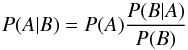 (1)holds, where P(A) and P(B) are unconditional probabilities for events A and B. In our application P(A | B) is the probability that model parameter τ falls within the interval τ...τ + dτ given the data. P(B | A) is the usual likelihood function, P(A) the so-called prior for τ, and P(B) the searched-for evidence of the model. The evidence is a model’s mean likelihood – averaged over the whole τ range and subject to the prior probability density – and as such, it measures the overall ability of the model to cope with the data. Since the prior probability must sum up to unity, the evidence diminishes if the parameter space expands beyond the space needed to cover the essential parts of the likelihood mountain.
We are interested here in evidence ratio, the Bayes factors. They allow a model ranking, i.e. to compare the explanatory powers of competitive models or hypotheses. The logarithm of age, τ = log e(t), is chosen, with t being the solar age, to make certain that the posterior for the age is compatible with the posterior of, say, the reciprocal of the age. With this decision the evidence does not depend on the unit of age. Accordingly, for P(A) a flat prior is assumed over the logarithm of age. All the other parameters of the solar model – the initial helium fraction Y0, the mixing length parameter, and the initial (Z/X)0 value – are adjusted in order to reproduce measured radius, effective temperature, and Z/X ratio at the surface. We do not attempt to derive credibility intervals for Y0, (Z/X)0, and the mixing length parameter, because they are obtained analytically, i.e., by means of the standard Newton-Raphson procedure embedded in the solar model calibration.
In actual calculations the likelihood function P(B | A) is often expressed by a Gaussian. In particular, if di = r02(n) are the observed data (n = i + 8,i = 1...N), mi the theoretical model values, and σi the errors, it reads as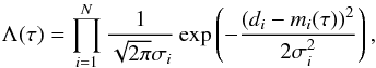 (2)with τ being log e(t) and N = 17. An observed quantity, di = r02(i + 8), is the ratio of two Gaussians that results, strictly speaking, in a Cauchy-like distribution3, not a Gaussian. With respect to the following likelihood function, which is based on Eq. (2), and for the sake of consistency, we decided, however, to compute the σi’s according to Gauss’s linearized error propagation rule.
Although Broomhall et al. (2009) have carefully taken the systematic error induced by solar activity into account, it is tempting to enhance the robustness of the age estimates by averaging over the errors, thereby obeying Jeffreys’ 1 /σ prior. In this way an error-integrated likelihood is obtained, which relies still on the Gaussianity assumption: ![\begin{equation} \Lambda^\prime = \int_0^\infty \hspace{-5pt}\Lambda\,{{\rm d}\sigma\over\sigma} = {\Gamma\left(N/2\right)\over 2\,\left(\pi N\right)^{N/2}}{1\over\left[\prod_{i=1}^{N} s_i\right] \left[{1\over N}\sum_{i=1}^N\left({d_i-m_i}\over s_i\right)^2\right]^{N/2}}, \label{l2} \end{equation}](/articles/aa/full_html/2015/08/aa26419-15/aa26419-15-eq48.png) (3)where σi = si·σ, and relative errors si are normalized according to
(3)where σi = si·σ, and relative errors si are normalized according to  , with
  the weights.
We also consider the median likelihood, which is constructed from the binomial distribution and ignores any information with regard to measurements errors. It only assumes that both positive and negative deviations di−mi have equal probability. It reads as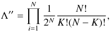 (4)with K the number of events with di ≥ mi (or di ≤ mi).
The evidence is the mean likelihood over parameter space; that is to say, in the case of a flat prior for τ = log e(t), 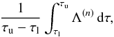 (5)where the interval τu−τl is the same in all cases where, when considered otherwise, the communicated Bayes factors would render useless.
4. Results
To properly resolve Λ(τ), the τ domain was covered by 80 equidistant grid points. We checked that our results are substantially insensitive to a further refinement of the grid. (The achieved log time resolution is, if expressed in a musician’s language, a little bit better than one cent.) The computation of the eigenfrequencies has been performed with the latest version of the public pulsation code, GYRE4, which employs a new Magnus multiple-shooting scheme, as described in detail in Townsend & Teitler (2013). For consistency we have thus implemented the 2010 CODATA also in GYRE. The results, ages, and Bayes factors are depicted in Tables 1–3 for the three likelihood functions (2)−(4) considered.
First, we note that the use of a significantly longer data set (Broomhall et al. 2009), in combination with a Gaussian likelihood (2), has provided us with a much sharper solar age estimate if compared to previous studies (Doğan et al. 2010; Christensen-Dalsgaard 2009); models obtained with Irwin EOS generally perform better than models with OPAL EOS, while the evidence for models with NACRE and Adelberger et al. (2011) reaction rates differ only marginally. Only Adelberger et al. (2011) reaction rates, combined with an Irwin EOS result in a helioseismic age t⊙, are consistent with the meteoritic one within 1σ.
The main reason for the age difference between models with NACRE and Adelberger et al. (2011) reaction rates is the value of the astrophysical Spp(0)-factor for the pp-fusion cross-section. The NACRE collaboration adopts Spp = 3.89 × 10⁻²⁵ MeVb, while Adelberger et al. (2011) adopt Spp = 4.01 × 10⁻²⁵ MeVb. As a consequence, the helioseismic age tends to be longer for the NACRE rates because of the reduced efficiency of the pp reactions.
Using the 2010 CODATA does not produce a significant impact on the solar age determination. On the other hand, if we consider for the OPAL +NACRE case in Table 1, which is the old CODATA value for Newton’s constant G = 6.67232 × 10⁻⁸ cm3 g-1 s-2, we find t⊙ = 4.696 ± 0.006 Gyr and a Bayes factor that is two orders of magnitude larger. This value for the solar age is consistent within one 1σ with the value of t⊙ = 4.62 ± 0.08 Gyr found by Doğan et al. (2010) (including PMS evolution), which was obtained with a much shorter BiSON data set.
In the case of the error-integrated likelihood (3), the expectation values of the solar age are reported in Table 2. They are basically the same as in the former (Gaussian) case (Table 1), but the uncertainties are at least a factor two larger. Of course, this is due to the extreme stance that even the magnitude of the error σ in (3) is assumed to be unknown.
Even more robust ages estimates are presented in Table 3. In median statistics, nothing is assumed about the shape of the symmetric error distribution. The expectation values of the solar age are systematically lower by up to 10 Myr as compared with the two other cases where the Gaussianity of the errors is presumed. The credibility regions are up to seven times larger than in the case of a Gaussian likelihood with trusted errors. More important, in terms of Bayes factors, all models now perform equally well!
5. Conclusions
Bayes factors are powerful indicators when it comes to quantifying the ability of solar models differing in input physics to cope with published “quiet Sun” frequency separation ratios. If one trusts the common Gaussianity assumption, models using the Irwin EOS perform best. Abandoning any error information, to be on the safe side, leads to inconclusive results with respect to Bayes factors (cf. Table 3), which stresses the importance of evaluating the trustworthiness of the error estimates that enter into Eqs. (2) and (3).
If we assume a Gaussian error distrobution, only models with Irwin EOS agree with the meteoritic age. Moreover, their Bayesian evidence exceeds those with an OPAL EOS by at least four orders of magnitude (cf. Table 2). With the Adelberger et al. reaction rates, the solar age proves to be even more consistent with the meteoritic age.
Incorporation of PMS evolution is essential because the standard deviation of the age estimation, ≤10 Myr in the case of Irwin EOS, is less than the 40–50 Myr time span of the PMS phase. Moreover, our helioseismic age is consistent with the notion of a birth line, since our starting PMS models are only 2 Myr distant from the birth line location. The switch from old CODATA to 2010 CODATA values does not effect the age estimate significantly, in contrast to the model’s evidence, at least if the published errors are taken seriously.
These conclusions are obtained using the “old” Grevesse & Noels (1993) with (Z/X)⊙ = 0.0245 at the surface. It is worth mentioning that the so-called “new abundances”, for
which (Z/X)⊙ = 0.0178 (Asplund et al. 2009), would lead to completely inconsistent values of the solar age and Bayes factors reduced by many orders of magnitude as indicated by the corresponding row entries in Tables 1 and 2.
One can indeed substitute Eq. (2) by the correct expression. The corresponding ages and their standard deviations are indistinguishable from the values communicated in Table 1. However, as the distribution is a “fat-tailed” one, all Bayes factors but one (that normalized to unity) are somewhat enhanced: in the worst case (“Irwin+AdelR+Asplund”) by 44 per cent, in all other cases by up to 14 per cent. More important, the ranking is not affected.
Acknowledgments
A.B. would like to thank Gianni Strazzulla and Brandon Johnson for enlightening discussions about calcium-aluminum-rich inclusions and the meteoritic age of the solar system.
References
- Adelberger, E. G., García, A., Robertson, R. G. H., et al. 2011, Rev. Mod. Phys., 83, 195 [NASA ADS] [CrossRef] [Google Scholar]
- Amelin, Y., Krot, A. N., Hutcheon, I. D., & Ulyanov, A. A. 2002, Science, 297, 1678 [NASA ADS] [CrossRef] [PubMed] [Google Scholar]
- Angulo, C., Arnould, M., Rayet, M., et al. 1999, Nucl. Phys. A, 656, 3 [NASA ADS] [CrossRef] [Google Scholar]
- Asplund, M., Grevesse, N., Sauval, A. J., & Scott, P. 2009, ARA&A, 47, 481 [NASA ADS] [CrossRef] [Google Scholar]
- Bahcall, J. N., Pinsonneault, M. H., & Wasserburg, G. J. 1995, Rev. Mod. Phys., 67, 781 [NASA ADS] [CrossRef] [Google Scholar]
- Bazot, M., Bourguignon, S., & Christensen-Dalsgaard, J. 2012, MNRAS, 427, 1847 [NASA ADS] [CrossRef] [Google Scholar]
- Bonanno, A., Murabito, A. L., & Paternò, L. 2001, A&A, 375, 1062 [NASA ADS] [CrossRef] [EDP Sciences] [Google Scholar]
- Bonanno, A., Schlattl, H., & Paternò, L. 2002, A&A, 390, 1115 [NASA ADS] [CrossRef] [EDP Sciences] [MathSciNet] [Google Scholar]
- Bouvier, A., & Wadhwa, M. 2010, Nature Geoscience, 3, 637 [CrossRef] [Google Scholar]
- Broomhall, A.-M., Chaplin, W. J., Davies, G. R., et al. 2009, MNRAS, 396, L100 [NASA ADS] [CrossRef] [Google Scholar]
- Cassisi, S., Salaris, M., & Irwin, A. W. 2003, ApJ, 588, 862 [NASA ADS] [CrossRef] [Google Scholar]
- Christensen-Dalsgaard, J. 2009, in IAU Symp. 258, eds. E. E. Mamajek, D. R. Soderblom, & R. F. G. Wyse, 431 [Google Scholar]
- Connelly, J. N., Bizzarro, M., Krot, A. N., et al. 2012, Science, 338, 651 [NASA ADS] [CrossRef] [Google Scholar]
- Cox, A. N. 2000, Allen’s astrophysical quantities (Springer) [Google Scholar]
- Doğan, G., Bonanno, A., & Christensen-Dalsgaard, J. 2010, in press, HELAS IV Conference [arXiv:1004.2215] [Google Scholar]
- Dziembowski, W. A., Fiorentini, G., Ricci, B., & Sienkiewicz, R. 1999, A&A, 343, 990 [NASA ADS] [Google Scholar]
- Ferguson, J. W., Alexander, D. R., Allard, F., et al. 2005, ApJ, 623, 585 [NASA ADS] [CrossRef] [Google Scholar]
- Gough, D. O. 2001, in Astrophysical Ages and Times Scales, eds. T. von Hippel, C. Simpson, & N. Manset, ASP Conf. Ser., 245, 31 [Google Scholar]
- Gough, D. O. 2012, in Progress in Solar/Stellar Physics with Helio- and Asteroseismology, eds. H. Shibahashi, M. Takata, & A. E. Lynas-Gray, ASP Conf. Ser., 462, 429 [Google Scholar]
- Gough, D. O., & Novotny, E. 1990, Sol. Phys., 128, 143 [Google Scholar]
- Grevesse, N., & Noels, A. 1993, in Origin and Evolution of the Elements, eds. N. Prantzos, E. Vangion-Flam, & M. Casse, Conf. Ser., 245, 14 [Google Scholar]
- Gruberbauer, M., & Guenther, D. B. 2013, MNRAS, 432, 417 [NASA ADS] [CrossRef] [Google Scholar]
- Gruberbauer, M., Guenther, D. B., MacLeod, K., & Kallinger, T. 2013, MNRAS, 435, 242 [NASA ADS] [CrossRef] [Google Scholar]
- Haberreiter, M., Schmutz, W., & Kosovichev, A. G. 2008, ApJ, 675, L53 [NASA ADS] [CrossRef] [Google Scholar]
- Houdek, G., & Gough, D. O. 2011, MNRAS, 418, 1217 [NASA ADS] [CrossRef] [Google Scholar]
- Hummer, D. G., & Mihalas, D. 1988, ApJ, 331, 794 [NASA ADS] [CrossRef] [Google Scholar]
- Iglesias, C. A., & Rogers, F. J. 1996, ApJ, 464, 943 [NASA ADS] [CrossRef] [Google Scholar]
- Jacobsen, B., Yin, Q.-z., Moynier, F., et al. 2008, Earth Plan. Sci. Lett., 272, 353 [Google Scholar]
- Jacobsen, B., Yin, Q.-Z., Moynier, F., et al. 2009, Earth Plan. Sci. Lett., 277, 549 [NASA ADS] [CrossRef] [Google Scholar]
- Kjeldsen, H., Bedding, T. R., & Christensen-Dalsgaard, J. 2008, ApJ, 683, L175 [NASA ADS] [CrossRef] [Google Scholar]
- Morel, P., Provost, J., & Berthomieu, G. 2000, A&A, 353, 771 [NASA ADS] [Google Scholar]
- Otí Floranes, H., Christensen-Dalsgaard, J., & Thompson, M. J. 2005, MNRAS, 356, 671 [NASA ADS] [CrossRef] [Google Scholar]
- Quirion, P.-O., Christensen-Dalsgaard, J., & Arentoft, T. 2010, ApJ, 725, 2176 [NASA ADS] [CrossRef] [Google Scholar]
- Reese, D. R., Marques, J. P., Goupil, M. J., Thompson, M. J., & Deheuvels, S. 2012, A&A, 539, A63 [NASA ADS] [CrossRef] [EDP Sciences] [Google Scholar]
- Rogers, F. J., & Nayfonov, A. 2002, ApJ, 576, 1064 [Google Scholar]
- Rogers, F. J., Swenson, F. J., & Iglesias, C. A. 1996, ApJ, 456, 902 [NASA ADS] [CrossRef] [Google Scholar]
- Roxburgh, I. W., & Vorontsov, S. V. 2003, A&A, 411, 215 [NASA ADS] [CrossRef] [EDP Sciences] [Google Scholar]
- Stahler, S. W. 1983, ApJ, 274, 822 [NASA ADS] [CrossRef] [Google Scholar]
- Stahler, S. W., & Palla, F. 2004, The Formation of Stars (New-York Wiley-VCH) [Google Scholar]
- Townsend, R. H. D., & Teitler, S. A. 2013, MNRAS, 435, 3406 [NASA ADS] [CrossRef] [Google Scholar]
- Trotta, R. 2008, Cont. Phys., 49, 71 [NASA ADS] [CrossRef] [Google Scholar]
- Weiss, A., & Schlattl, H. 2008, Ap&SS, 316, 99 [NASA ADS] [CrossRef] [Google Scholar]
All Tables
Current usage metrics show cumulative count of Article Views (full-text article views including HTML views, PDF and ePub downloads, according to the available data) and Abstracts Views on Vision4Press platform.
Data correspond to usage on the plateform after 2015. The current usage metrics is available 48-96 hours after online publication and is updated daily on week days.
Initial download of the metrics may take a while.