| Issue |
A&A
Volume 580, August 2015
|
|
|---|---|---|
| Article Number | A76 | |
| Number of page(s) | 9 | |
| Section | Catalogs and data | |
| DOI | https://doi.org/10.1051/0004-6361/201526273 | |
| Published online | 05 August 2015 | |
Astrometric positions for 18 irregular satellites of giant planets from 23 years of observations ⋆,⋆⋆,⋆⋆⋆,⋆⋆⋆⋆
1
Observatório do Valongo/UFRJ,
Ladeira Pedro Antônio 43, CEP 20.,
080-090
Rio de Janeiro –,
RJ,
Brazil
e-mail:
This email address is being protected from spambots. You need JavaScript enabled to view it.
2
Observatório Nacional/MCT, R. General José Cristino 77, CEP,
20921-400
Rio de Janeiro –,
RJ,
Brazil
e-mail:
This email address is being protected from spambots. You need JavaScript enabled to view it.
3
Laboratório Interinstitucional de e-Astronomia – LIneA, Rua Gal.
José Cristino 77, Rio de Janeiro, RJ,
20921-400,
Brazil
4
Institut de mécanique céleste et de calcul des éphémérides –
Observatoire de Paris, UMR 8028 du CNRS, 77 av. Denfert-Rochereau, 75014
Paris,
France
e-mail:
This email address is being protected from spambots. You need JavaScript enabled to view it.
5
Federal University of Technology – Paraná
(UTFPR/DAFIS), Rua Sete de
Setembro, 3165, CEP 80230-901
Curitiba, PR, Brazil
6
Centro Universitário Estadual da Zona Oeste,
Av. Manual Caldeira de Alvarenga 1203, CEP
23.070-200
Rio de Janeiro
RJ,
Brazil
7
ESIGELEC-IRSEEM, Technopôle du Madrillet, Avenue
Galilée, 76801
Saint-Etienne du Rouvray,
France
Received: 7 April 2015
Accepted: 6 May 2015
Abstract
Context. The irregular satellites of the giant planets are believed to have been captured during the evolution of the solar system. Knowing their physical parameters, such as size, density, and albedo is important for constraining where they came from and how they were captured. The best way to obtain these parameters are observations in situ by spacecrafts or from stellar occultations by the objects. Both techniques demand that the orbits are well known.
Aims. We aimed to obtain good astrometric positions of irregular satellites to improve their orbits and ephemeris.
Methods. We identified and reduced observations of several irregular satellites from three databases containing more than 8000 images obtained between 1992 and 2014 at three sites (Observatório do Pico dos Dias, Observatoire de Haute-Provence, and European Southern Observatory – La Silla). We used the software Platform for Reduction of Astronomical Images Automatically (PRAIA) to make the astrometric reduction of the CCD frames. The UCAC4 catalog represented the International Celestial Reference System in the reductions. Identification of the satellites in the frames was done through their ephemerides as determined from the SPICE/NAIF kernels. Some procedures were followed to overcome missing or incomplete information (coordinates, date), mostly for the older images.
Results. We managed to obtain more than 6000 positions for 18 irregular satellites: 12 of Jupiter, 4 of Saturn, 1 of Uranus (Sycorax), and 1 of Neptune (Nereid). For some satellites the number of obtained positions is more than 50% of what was used in earlier orbital numerical integrations.
Conclusions. Comparison of our positions with recent JPL ephemeris suggests there are systematic errors in the orbits for some of the irregular satellites. The most evident case was an error in the inclination of Carme.
Key words: planets and satellites: general / planets and satellites: individual: Jupiter / planets and satellites: individual: Saturn / astrometry
Position tables are only available at the CDS via anonymous ftp to cdsarc.u-strasbg.fr (130.79.128.5) or via http://cdsarc.u-strasbg.fr/viz-bin/qcat?J/A+A/580/A76 and IAU NSDC database at www.imcce.fr/nsdc
Partially based on observations made at Laboratório Nacional de Astrofísica (LNA), Itajubá-MG, Brazil.
Partially based on observations through the ESO runs 079.A-9202(A), 075.C-0154, 077.C-0283 and 079.C-0345.
Partially based on observations made at Observatoire de Haute Provence (OHP), 04870 Saint-Michel l’observatoire, France.
© ESO, 2015
1. Introduction
The irregular satellites of the giant planets are smaller than the regular moons, having more eccentric, inclined, distant, and in most cases, retrograde orbits. Owing to their orbital configurations, it is largely accepted that these objects were captured in the early solar system (Sheppard & Jewitt 2003).
Because they are faint, the majority of these objects were only discovered in the last century1. They were never visited by a spacecraft, with the exception of Himalia, Phoebe, and Nereid, in a flyby by the Cassini space probe in 2000 for Himalia (Porco et al. 2003) and in 2004 for Phoebe (Desmars et al. 2013) and in a flyby by the Voyager 2 space probe in 1989 for Nereid (Smith et al. 1989). Even in situ, they were still opportunity target observations resulting in not optimal measurements, with size errors of 10 km for Himalia and 25 km for Nereid (Thomas et al. 1991). The exception is Phoebe with a very accurate measurement of size with a mean radius error of 0.7 km (Thomas 2010).
If these objects were captured, there remains the question of where they came from. Clark et al. (2005) show from imaging spectroscopy from Cassini that Phoebe has a surface probably covered by material from the outer solar system and Grav et al. (2003) show that the satellites of the Jovian Prograde Group Himalia have gray colors implying that their surfaces are similar to that of C-type asteroids. In that same work, the Jovian Retrograde Group Carme was found to have surface colors similar to the D-type asteroids as for the Hilda or Trojan families, while JXIII Kalyke has a redder color like Centaurs or trans-Neptunian objects (TNOs).
For Saturnian satellites, Grav & Bauer 2007 show by their colors and spectral slopes that these satellites contain a more or less equal fraction of C-, P-, and D-like objects, but SXXII Ijiraq is marginally redder than D-type objects. These works may suggest different origins for the irregular satellites.
In this context, we used three databases for deriving precise positions for the irregular satellites observed at the Observatório do Pico dos Dias (OPD; 1.6 m and 0.6 m telescopes, IAU code 874), the Observatoire Haute-Provence (OHP; 1.2 m telescope, IAU code 511), and the European Southern Observatory (ESO; 2.2 m telescope, IAU code 809). Many irregular satellites were observed between 1992 and 2014, covering a few orbital periods of these objects (12 satellites of Jupiter, 4 of Saturn, Sycorax of Uranus, and Nereid of Neptune).
Since their ephemerides are not very precise, predicting and observing stellar occultations are very difficult, and no observation of such an event for an irregular satellite is found in the literature. The precise star positions to be derived by the ESA astrometry satellite Gaia (de Bruijne 2012) will render better predictions with the only source of error being the ephemeris. The positions derived from our observations can be used in new orbital numerical integrations, generating more precise ephemerides.
The power of stellar occultations for observing relatively small diameter solar system objects is supported by recent works, such as the discovery of a ring system around the Centaur (10199) Chariklo (Braga-Ribas et al. 2014). Once irregular satellites start to be observed by this technique, it will be possible to obtain their physical parameters (shape, size, albedo, density) with unprecedented precision. For instance, in this case, sizes could be obtained with kilometer accuracy. The knowledge of these parameters would in turn bring valuable information for studying the capture mechanisms and origin of the irregular satellites.
The databases are described in Sect. 2. The astrometric procedures in Sect. 3. The obtained positions are presented in Sect. 4 and analyzed in Sect. 5. Conclusions are given in Sect. 6.
2. Databases
Our three databases consist of optical CCD images from many observational programs performed with different telescopes and detectors that target a variety of objects, among which are irregular satellites. The observations were made at three sites: OPD, OHP, and ESO. All together there are more than 8000 FITS images obtained in a large time span (1992−2014) for the irregular satellites. Since the OHP and mostly the OPD database registers were not well organized, we had to start from scratch and develop an automatic procedure to identify and filter only the images of interest, that is, for the irregular satellites. The instrument and image characteristics are described in the following sections.
2.1. OPD
The OPD database was produced at the Observatório do Pico dos Dias (OPD, IAU code 874, 45° 34′ 57″ W, 22° 32′ 04″ S, 1864 m)2, located at geographical longitude , in Brazil. The observations were made between 1992 and 2014 by our group in a variety of observational programs. Two telescopes of 0.6 m diameter (Zeiss and Boller & Chivens) and one 1.6 m diameter (Perkin-Elmer) were used for the observations. Identified were 5248 observations containing irregular satellites, with 3168 from the Boller & Chivens, 1967 from the Perkin-Elmer, and 113 from the Zeiss.
This is an inhomogeneous database with observations made with nine different detectors (see Table 1) and six different filters. The headers of most of the older FITS images had missing, incomplete, or incorrect coordinates or dates. In some cases, we could not identify the detector’s origin. The procedures used to overcome these problems are described in Sect. 3.
Characteristics of OPD detectors used in this work.
2.2. OHP
The instrument used at the OHP (IAU code 511, 5° 42′ 56.5″ E, 43° 55′ 54.7″N, 633.9 m)3 was the 1.2m-telescope in a Newton configuration. The focal length is 7.2 m. The observations were made between 1997 and 2008. During this time only one CCD detector 1024 × 1024 was used. The size of field is 12′ × 12′ with a pixel scale of 0.69″. From these observations, 2408 were identified containing irregular satellites.
2.3. ESO
Observations were made at the 2.2 m Max-Planck ESO (ESO2p2) telescope (IAU code 809, 70°44′1.5″ W, 29°15′31.8″ S, 2345.4 m)4 with the Wide Field Imager (WFI) CCD mosaic detector. Each mosaic is composed of eight CCDs of 7.5′ × 15′ (α, δ) sizes, resulting in a total coverage of 30′ × 30′ per mosaic. Each CCD has 4 k × 2 k pixels with a pixel scale of 0.238″. The filter used was a broad-band R filter (ESO#844) with λc = 651.725 nm and Δλ = 162.184 nm. The telescope was shifted between exposures in such a way that each satellite was observed at least twice in different CCDs.
The satellites were observed in 24 nights, divided in five runs between April 2007 and May 2009 in parallel with, and using the same observational and astrometric procedures of the program that observed stars along the sky path of TNOs to identify candidates for stellar occultation (see Assafin et al. 2010, 2012). A total of 810 observations were obtained for irregular satellites.
3. Astrometry
Almost all the frames were photometrically calibrated with auxiliary bias and flat-field frames by means of standard procedures using IRAF5 and, for the mosaics, using the esowfi (Jones & Valdes 2000) and mscred (Valdes 1998) packages. Some of the nights at OPD did not have bias and flat-field images so the correction was not possible.
The astrometric treatment was made with the Platform for Reduction of Astronomical Images Automatically (PRAIA; Assafin et al. 2011). The (x, y) measurements were performed with two-dimensional circular symmetric Gaussian fits within one full width half maximum (FWHM = seeing). Within one FWHM, the image profile is described well by a Gaussian profile, which is free of the wing distortions, which may jeopardize the determination of the center. PRAIA automatically recognizes catalog stars and determines (α, δ) with a user-defined model relating the (x, y) measured and (X, Y) standard coordinates projected in the sky tangent plane.
We used the UCAC4 (Zacharias et al. 2013) as the practical representative of the International Celestial Reference System (ICRS). For each frame, we used the six constants polynomial model to relate the (x, y) measurements with the (X, Y) tangent plane coordinates. For ESO, we followed the same astrometric procedures as described in detail in Assafin et al. (2012); the (x, y) measurements of the individual CCDs were precorrected by a field distortion pattern, and all positions coming from different CCDs and mosaics were then combined using a third degree polynomial model to produce a global solution for each night and field observed, and final (α, δ) object positions were obtained in the UCAC4 system.
In Table 2 we list the average mean error in α and δ for the reference stars obtained by telescope, the average (x, y) measurement errors of the Gaussian fits described above, and the mean number of UCAC4 stars used by frame. For all databases, about 20% of outlier reference stars were eliminated for presenting (O−C) position residuals higher than 120 mas in the (α, δ) reductions.
Astrometric (α, δ) reduction by telescope.
To help identify the satellites in the frames and derive the ephemeris for the instants of the observations for comparisons (see Sect. 5), we used the kernels from SPICE/JPL6. Emelyanov & Arlot (2008) and references therein also provided ephemeris of similar quality for the irregular satellites. For instance, for Himalia, which has relatively good orbit solutions, the ephemerides differ by less than 20 mas, and in the case of less-known orbits, like Ananke, the differences are less than 90 mas. We chose to use the JPL ephemeris because they used more recent observations (see Jacobson et al. 2012). The JPL ephemeris that represented the Jovian satellites in this work was the DE421 + JUP300. For the Saturnian satellites, the ephemeris was DE421 + SAT359 to Hyperion, Iapetus, and Phoebe and DE421 + SAT361 to Albiorix, Siarnaq, and Paaliaq. The DE421 + URA095 was used for Sycorax and DE421 + NEP081 for Nereid. More recent JPL ephemeris versions became available after completion of this work, but this did not affect the results.
Astrometric (α, δ) reduction for each satellite observed with the Perkin-Elmer telescope.
In the OPD database, there were some images (mostly the older ones) with missing coordinates or the wrong date in their headers. In the case of missing or incorrect coordinates, we adopted the ephemeris as the central coordinates of the frames. When the time was not correct, the field of view identification failed. In this case, a search for displays of wrong date (year) was performed. Problems like registering local time instead of UTC were also identified and corrected.
In all databases, for each night a sigma-clipping procedure was performed to eliminate discrepant positions (outliers). A threshold of 120 mas and a deviation of more than 2.5 sigma from the nightly average ephemeris offsets were adopted.
From Tables 3 to 7 we list the average dispersion (standard deviation) of the position offsets with regard to the ephemeris for α and δ obtained by telescope for each satellite. The final number of frames, number of nights (in parenthesis), the mean number of UCAC4 stars used in the reduction and the approximate V magnitude are also given. The dashed lines separate the satellites from different families with similar orbital parameters: Himalia Group (Himalia, Elara, Lysithea, and Leda), Pasiphae Group (Pasiphae, Callirrhoe, and Megaclite), and Ananke Group (Ananke and Praxidike). Carme and Sinope are the only samples of their groups. From Saturn, Siarnaq and Paaliaq are from the Inuit Group while Phoebe and Albiorix are the only samples in their groups.
The differences in the dispersion of the ephemeris offsets of the same satellite for distinct telescopes seen in Tables 3 to 7 are caused by the different distribution of observations along the orbit for each telescope. This can be seen in Fig. 1 for Carme and Fig. 2 for Pasiphae and for all objects in Appendix A. Since the observations cover different segments of the orbit, the dispersion of the offsets may vary for different telescopes for a single satellite, with larger covered segments usually implying larger dispersions and vice versa. For Nereid, due to its high eccentric orbit, the observations are located between 90° and 270° of true anomaly where Nereid remains most of the time.
Astrometric (α, δ) reduction for each satellite observed with the Boller & Chivens telescope.
Astrometric (α, δ) reduction for each satellite observed with the Zeiss telescope.
Astrometric (α, δ) reduction for each satellite observed with the OHP telescope.
Astrometric (α, δ) reduction for each satellite observed with the ESO telescope.
No solar phase correction was applied to the positions. For the biggest irregular satellite of Jupiter, Himalia, it was verified that the maximum deviation in the position due to phase angle is 1.94 mas using the phase correction described in Lindegren (1977). For the other satellites, which are smaller objects, this deviation is even smaller. Since our position error is one order of magnitude higher, this effect was neglected.
4. Satellite positions
The final set of positions of the satellites consists in 6523 cataloged positions observed between 1992 and 2014 for 12 satellites of Jupiter, 4 of Saturn, 1 of Uranus, and 1 of Neptune. The topocentric positions are in the ICRS. The catalogs (one for each satellite) contain epoch of observations, the position error, filter used, estimated magnitude (from point spread function fitting) and telescope origin. The magnitude errors can be as high as 1 mag; they are not photometrically calibrated and should be used with care. The position errors were estimated from the dispersion of the ephemeris offsets of the night of observation of each position. Thus, these position errors are probably overestimated because there must be ephemeris errors present in the dispersion of the offsets. These position catalogs are freely available in electronic form at the CDS (see a sample in Table 8) and at the IAU NSDC database7.
The number of positions acquired is significant compared to the number used in the numerical integration of orbits by the JPL (Jacobson et al. 2012) as shown in Table 9.
CDS data table sample for Himalia.
Comparison between the number of positions obtained in our work with the number used in the numerical integration of orbits by the JPL as published by Jacobson et al. (2012).
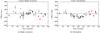 |
Fig. 1 Mean ephemeris offsets and dispersions (1 sigma error bars) in the coordinates of Carme taken night by night by true anomaly for each telescope. The red square is for the observations with the Perkin-Elmer telescope from OPD, the blue circle for Boller & Chivens, the magenta triangle down for Zeiss, the black triangle up for OHP and the green star for ESO. |
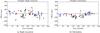 |
Fig. 2 Same as in Fig. 1 for Pasiphae. |
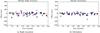 |
Fig. A.1 Mean ephemeris offset and dispersion (1 sigma error bars) in the coordinates of Himalia taken night by night as a function of true anomaly. |
5. Comparison with ephemeris
Intending to see the potential of our results to improve the orbit of the irregular satellites observed, we analyzed the offsets of our positions with regard to the ephemeris mentioned in Sect. 3. Taking Carme as example, we plot the mean ephemeris offsets for each night in Fig. 1 and their dispersions (one sigma error bars) as a function of the true anomaly in right ascension (1a) and declination (1b). Figure 1b clearly shows a systematic error in declination. When Carme is close to its apojove (true anomaly =180°), its offsets are more likely to be more negative than those close to its perijove (true anomaly =0°). The offsets obtained from observations by four telescopes using different cameras and filters are in good agreement, meaning that there is an error in the ephemeris of Carme, most probably due to an error in its orbital inclination.
This pattern in declination was also seen for other satellites like Pasiphae (Fig. 2) and Ananke (plots for other satellites with significant number of observations can be seen in Appendix A). For some satellites, the orbital coverage is not enough to clearly indicate the presence of systematic errors in specific orbital elements. However, after comparing the internal position mean errors of the reductions (Table 2) with the external position errors estimated from the dispersion of the ephemeris offsets (Tables 3 to 7), we see position error values that are much higher than expected from the mean errors. This means that besides some expected astrometric errors, significant ephemeris errors must also be present.
6. Conclusions
We managed a large database with FITS images acquired by five telescopes in three sites between 1992 and 2014. From that, we identified 8466 observations of irregular satellites, from which we managed to obtain 6523 suitable astrometric positions, giving a total of 3666 positions for 12 satellites of Jupiter, 1920 positions for 4 satellites of Saturn, 35 positions for Sycorax (Uranus) and 902 positions for Nereid (Neptune).
The positions of all the objects were determined using the PRAIA package. The package was suited to coping with the huge number of observations and with the task of identifying the satellites within the database. PRAIA tasks were also useful for dealing with the missing or incorrect coordinate and time stamps present mostly in the old observations.
The UCAC4 was used as the reference frame. Based on the comparisons with ephemeris, we estimate that the position errors are about 60 mas to 80 mas depending on the satellite brightness. For some satellites the number of positions obtained in this work is comparable to the number used in the numerical integration of orbits by the JPL (Jacobson et al. 2012) (see Table 9). For instance, the number of new positions for Himalia is about 70% of the number used in the numerical integation of orbits by JPL. Systematic errors in the ephemeris were found for at least some satellites (Ananke, Carme, Elara and Pasiphae). In the case of Carme, we showed an error in the orbital inclination (see Fig. 1).
The positions derived in this work can be used in new orbital numerical integrations, generating more precise ephemerides. Stellar occultations by irregular satellites could then be predicted better. Based on this work, our group has already computed occultation predictions for the eight major irregular satellites of Jupiter. These predictions will be published in a forthcoming paper.
Website: www.obs-hp.fr/guide/t120.shtml – in French
Website: http://iraf.noao.edu/
Acknowledgments
A.R.G.J. acknowledges the financial support of CAPES. M.A. is grateful to the CNPq (Grants 473002/2013-2 and 308721/2011-0) and FAPERJ (Grant E-26/111.488/2013). R.V.M. acknowledges the following grants: CNPq-306885/2013, Capes/Cofecub-2506/2015, Faperj/PAPDRJ-45/2013. J.-E.A. is grateful to the “Programme National de Planétologie” of INSU-CNRS-CNES for its financial support. J.I.B. Camargo acknowledges CNPq for a PQ2 fellowship (process number 308489/2013-6). F.B.R. acknowledges PAPDRJ-FAPERJ/CAPES E-43/2013 number 144997, E-26/101.375/2014. B.E.M. is grateful for the financial support of CAPES.
References
- Assafin, M., Camargo, J. I. B., Vieira Martins, R., et al. 2010, A&A, 515, A32 [NASA ADS] [CrossRef] [EDP Sciences] [Google Scholar]
- Assafin, M., Vieira Martins, R., Camargo, J. I. B., et al. 2011, in Gaia follow-up network for the solar system objects: Gaia FUN-SSO workshop Proc. IMCCE -Paris Observatory, France, Nov. 29 – Dec. 1, 2010, eds. P. Tanga, & W. Thuillot, 85 [Google Scholar]
- Assafin, M., Camargo, J. I. B., Vieira Martins, R., et al. 2012, A&A, 541, A142 [NASA ADS] [CrossRef] [EDP Sciences] [Google Scholar]
- Braga-Ribas, F., Sicardy, B., Ortiz, J. L., et al. 2014, Nature, 508, 72 [NASA ADS] [CrossRef] [Google Scholar]
- Clark, R. N., Brown, R. H., Jaumann, R., et al. 2005, Nature, 435, 66 [NASA ADS] [CrossRef] [PubMed] [Google Scholar]
- de Bruijne, J. H. J. 2012, Astrophys. Space Sci., 341, 31 [Google Scholar]
- Desmars, J., Li, S. N., Tajeddine, R., Peng, Q. Y., & Tang, Z. H. 2013, A&A, 553, A36 [NASA ADS] [CrossRef] [EDP Sciences] [Google Scholar]
- Emelyanov, N. V., & Arlot, J.-E. 2008, A&A, 487, 759 [NASA ADS] [CrossRef] [EDP Sciences] [Google Scholar]
- Grav, T., & Bauer, J. 2007, Icarus, 191, 267 [NASA ADS] [CrossRef] [Google Scholar]
- Grav, T., Holman, M. J., Gladman, B. J., & Aksnes, K. 2003, Icarus, 166, 33 [NASA ADS] [CrossRef] [Google Scholar]
- Jacobson, R., Brozovi, M., Gladman, B., et al. 2012, AJ, 144, 132 [NASA ADS] [CrossRef] [Google Scholar]
- Jones, H., & Valdes, F. 2000, in Handling ESO WFI Data With IRAF, ESO Document number 2p2-MAN-ESO-22200-00002 [Google Scholar]
- Lindegren, L. 1977, A&A, 57, 55 [NASA ADS] [Google Scholar]
- Porco, C. C., West, R. A., McEwen, A., et al. 2003, Science, 299, 1541 [NASA ADS] [CrossRef] [PubMed] [Google Scholar]
- Sheppard, S. S., & Jewitt, D. C. 2003, Nature, 423, 261 [NASA ADS] [CrossRef] [Google Scholar]
- Smith, B. A., Soderblom, L. A., Banfield, D., et al. 1989, Science, 246, 1422 [NASA ADS] [CrossRef] [PubMed] [Google Scholar]
- Thomas, P. 2010, Icarus, 208, 395 [NASA ADS] [CrossRef] [Google Scholar]
- Thomas, P., Veverka, J., & Helfenstein, P. 1991, J. Geophys. Res., 96, 19253 [NASA ADS] [CrossRef] [Google Scholar]
- Valdes, F. G. 1998, in The IRAF Mosaic Data Reduction Package in Astronomical Data Analysis Software and Systems VII, eds. R. Albrecht, R. N. Hook, & H. A. Bushouse, ASP Conf. Ser., 145, 53 [Google Scholar]
- Zacharias, N., Finch, C. T., Girard, T. M., et al. 2013, AJ, 145, 44 [NASA ADS] [CrossRef] [EDP Sciences] [Google Scholar]
Appendix A: Ephemeris offsets as a function of true anomaly for all observed irregular satellites
The distribution of ephemeris offsets along the orbit of the satellites are shown below. The red square is for the observations with the Perkin-Elmer telescope from OPD, the blue circle for Boller & Chivens, the magenta triangle down for Zeiss, the black triangle up for OHP and the green star for ESO. For Carme and Pasiphae see Figs. 1 and 2 in Sect. 5.
All Tables
Astrometric (α, δ) reduction for each satellite observed with the Perkin-Elmer telescope.
Astrometric (α, δ) reduction for each satellite observed with the Boller & Chivens telescope.
Astrometric (α, δ) reduction for each satellite observed with the Zeiss telescope.
Astrometric (α, δ) reduction for each satellite observed with the OHP telescope.
Comparison between the number of positions obtained in our work with the number used in the numerical integration of orbits by the JPL as published by Jacobson et al. (2012).
All Figures
|
Fig. 1 Mean ephemeris offsets and dispersions (1 sigma error bars) in the coordinates of Carme taken night by night by true anomaly for each telescope. The red square is for the observations with the Perkin-Elmer telescope from OPD, the blue circle for Boller & Chivens, the magenta triangle down for Zeiss, the black triangle up for OHP and the green star for ESO. |
| In the text | |
|
Fig. 2 Same as in Fig. 1 for Pasiphae. |
| In the text | |
|
Fig. A.1 Mean ephemeris offset and dispersion (1 sigma error bars) in the coordinates of Himalia taken night by night as a function of true anomaly. |
| In the text | |
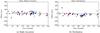 |
Fig. A.2 Same as in Fig. A.1 for Elara. |
| In the text | |
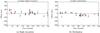 |
Fig. A.3 Same as in Fig. A.1 for Lysithea. |
| In the text | |
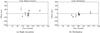 |
Fig. A.4 Same as in Fig. A.1 for Leda. |
| In the text | |
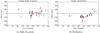 |
Fig. A.5 Same as in Fig. A.1 for Ananke. |
| In the text | |
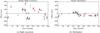 |
Fig. A.6 Same as in Fig. A.1 for Sinope. |
| In the text | |
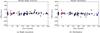 |
Fig. A.7 Same as in Fig. A.1 for Phoebe. |
| In the text | |
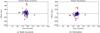 |
Fig. A.8 Same as in Fig. A.1 for Nereid. |
| In the text | |
Current usage metrics show cumulative count of Article Views (full-text article views including HTML views, PDF and ePub downloads, according to the available data) and Abstracts Views on Vision4Press platform.
Data correspond to usage on the plateform after 2015. The current usage metrics is available 48-96 hours after online publication and is updated daily on week days.
Initial download of the metrics may take a while.